
16
FEM in Three Dimensions
16.1 Creating Three-Dimensional Meshes
Our first task in developing three-dimensional (3d) FEM capability is to generate 3d meshes to describe our geometries. Fortunately, gmsh is well equipped to do this, with its two-dimensional (2d) meshing capabilities extending directly into three dimensions. As in the case of 2d meshes, there are many ways to generate a given geometry in three dimensions. In this chapter we will consider only one of these approaches. The gmsh documentation and many online sources should be consulted for a comprehensive discussion of this topic.
A problem that we will encounter using unstructured 3d meshes is that visualizing what we have done can be difficult; there is simply too much going on. In the examples in this chapter, many of the figures of meshed structures were generated using low-resolution meshing. This is necessary to make these figures at all useful. The .geo file accompanying these examples will show the resolution used to generate any results quoted from the FEM analysis. Also, the gmsh ability to rotate a figure in space was utilized in generating some of the figures. Since the rotation chosen for a figure was arbitrary (it looked good), details of the rotation are not given.
The gmsh script struct16_1.geo shows the construction of a cube:
// struct16_1.geo
// first experiments with 3D

lc = 1;

Point(1) = {-.5, -.5, -.5, lc};
Point(2) = {.5, -.5, -.5, lc};
Point(3) = {.5, .5, -.5, lc};
Point(4) = {-.5, .5, -.5, lc};

Point(5) = {-.5, -.5, .5, lc};
Point(6) = {.5, -.5, .5, lc};
Point(7) = {.5, .5, .5, lc};
Point(8) = {-.5, .5, .5, lc};

Line(1) = {1, 2};
Line(2) = {2, 3};
Line(3) = {3, 4};
Line(4) = {4, 1};

Line(5) = {5, 6};
Line(6) = {6, 7};
Line(7) = {7, 8};
Line(8) = {8, 5};

Line(9) = {1, 5};
Line(10) = {2, 6};
Line(11) = {3, 7};
Line(12) = {4, 8};

Line Loop(1) = {1, 2, 3, 4}; // front
Line Loop(2) = {1, 10, -5, -9}; // bottom
Line Loop(3) = {-3, 11, 7, -12}; // top
Line Loop(4) = {5, 6, 7, 8}; // back
Line Loop(5) = {-9, -4, 12, 8}; // left
Line Loop(6) = {-10, 2, 11, -6}; // right

Plane Surface(1) = {1};
Plane Surface(2) = {2};
Plane Surface(3) = {3};
Plane Surface(4) = {4};
Plane Surface(5) = {5};
Plane Surface(6) = {6};

Surface Loop(1) = {1, 2, 3, 4, 5, 6};
Volume(1) = {1};

//Volume(1) = {10, 20, 30, 40, 50, 60};
Examining this file, first we see the eight points that define the vertices of the cube. Then we see the 12 lines that connect these points to form the edges of the cube, followed by the six line loops that make up the edges of the surfaces of the cube. Note the negative numbers in some of the line loop definitions. A line loop must “walk its way” around a surface, with all lines interconnected in a tail-to-head configuration (first defining number to second defining number). If a line is defined incorrectly, simply putting a minus sign in front of its number in the line loop definition has the effect of reversing the head and tail of the line.
Continuing, we see the six plane surface definitions for the six faces of the cube. We ultimately see two lines that we haven’t seen before. The surface loop definition connects the six surfaces defined by line loops into one closed surface, just as the line loop definition connects lines into a closed loop. Finally, the volume definition identifies the volume enclosed by the surface loop, our cube.
Meshing the volume is accomplished with the Mesh – 3D command. The result of this is shown in Figure 16.1. Several points to note are:
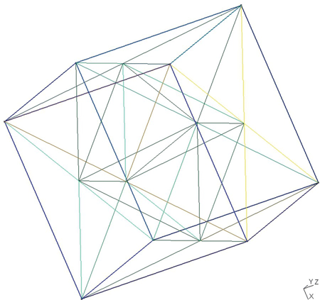
FIGURE 16.1 A meshed cube.
- Figure 16.1 is a rotated view of the figure that the
gmshscreen first shows, as discussed above. This rotation is accomplished by grabbing the small coordinate axis in the lower right corner of thegmshscreen and dragging it around. The original orientation can be returned by clicking on the Z in the lower left corner of thegmshscreen. Clicking on Z means that we are looking down at a transparent X–Y plane. Similarly, the X or Y immediately to the left of the Z can be clicked on. In this simple example all three choices will yield the same picture. - As seen in the rotated figure,
gmshhas zoned the cube into a collection of tetrahedrons. A tetrahedron is a four-sided figure in which each face is a triangle. Using tetrahedrons as our 3d elements is not a necessary choice, but it is the simplest way to move from triangles in two dimensions. In this simple example the grid appears to be structured. This is the result of the highly symmetric geometry of the cube, not an inherent property of gmsh. - The resolution chosen is very low.
- This cube is an acceptable geometry for a bounding electrode box or for a cubical electrode inside some bounding region, but by itself there is no possible electrostatic FEM analysis. The surface of the cube will be a boundary condition, and we need (at least) two different boundary conditions (voltages) before there is a voltage distribution to find.
The gmsh script struct16_2.geo is a geometry description almost ready for FEM analysis:
// Struct16_2.geo
// Inner and outer box experiment

lc = 1;

// inner box

Point(1) = {-.5, -.5, -.5, lc};
Point(2) = {.5, -.5, -.5, lc};
Point(3) = {.5, .5, -.5, lc};
Point(4) = {-.5, .5, -.5, lc};

Point(5) = {-.5, -.5, .5, lc};
Point(6) = {.5, -.5, .5, lc};
Point(7) = {.5, .5, .5, lc};
Point(8) = {-.5, .5, .5, lc};

Line(1) = {1, 2};
Line(2) = {2, 3};
Line(3) = {3, 4};
Line(4) = {4, 1};

Line(5) = {5, 6};
Line(6) = {6, 7};
Line(7) = {7, 8};
Line(8) = {8, 5};

Line(9) = {1, 5};
Line(10) = {2, 6};
Line(11) = {3, 7};
Line(12) = {4, 8};

Line Loop(1) = {1, 2, 3, 4}; // front
Line Loop(2) = {1, 10, -5, -9}; // bottom
Line Loop(3) = {-3, 11, 7, -12}; // top
Line Loop(4) = {5, 6, 7, 8}; // back
Line Loop(5) = {-9, -4, 12, 8}; // left
Line Loop(6) = {-10, 2, 11, -6}; // right

Plane Surface(1) = {1};
Plane Surface(2) = {2};
Plane Surface(3) = {3};
Plane Surface(4) = {4};
Plane Surface(5) = {5};
Plane Surface(6) = {6};

Surface Loop(1) = {1, 2, 3, 4, 5, 6};

// outer box

Point(100) = {-1, -1, -1, lc};
Point(200) = {1, -1, -1, lc};
Point(300) = {1, 1, -1, lc};
Point(400) = {-1, 1, -1, lc};

Point(500) = {-1, -1, 1, lc};
Point(600) = {1, -1, 1, lc};
Point(700) = {1, 1, 1, lc};
Point(800) = {-1, 1, 1, lc};

Line(100) = {100, 200};
Line(200) = {200, 300};
Line(300) = {300, 400};
Line(400) = {400, 100};

Line(500) = {500, 600};
Line(600) = {600, 700};
Line(700) = {700, 800};
Line(800) = {800, 500};

Line(900) = {100, 500};
Line(1000) = {200, 600};
Line(1100) = {300, 700};
Line(1200) = {400, 800};

Line Loop(100) = {100, 200, 300, 400}; // front
Line Loop(200) = {100, 1000, -500, -900}; // bottom
Line Loop(300) = {-300, 1100, 700, -1200}; // top
Line Loop(400) = {500, 600, 700, 800}; // back
Line Loop(500) = {-900, -400, 1200, 800}; // left
Line Loop(600) = {-1000, 200, 1100, -600}; // right

Plane Surface(100) = {100};
Plane Surface(200) = {200};
Plane Surface(300) = {300};
Plane Surface(400) = {400};
Plane Surface(500) = {500};
Plane Surface(600) = {600};

Surface Loop(100) = {100, 200, 300, 400, 500, 600};

Volume(1) = {100, 1};
Script struct16_2.geo extends struct16_1.geo in that now there are two cubes, a smaller cube centered inside a larger cube, as seen in Figure 16.2.
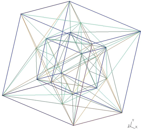
FIGURE 16.2 Two concentric cubes.
The volume statement in struct16_2.geo specifies the surface loop of the larger, outer cube followed by the surface loop of the smaller, inner cube. The resultant meshing treats the inner cube as a subtracted region and creates tetrahedrons only in the region between (and on) the two cube surfaces. This is exactly the meshing we want for treating this as an electrostatics problem where the two cube surfaces are electrodes (and the outer cube surface is a bounding surface). Once again, in this example the resolution of the meshing is kept very low so that the figure is comprehensible to the viewer. A careful examination of Figure 16.2 will reveal that the resolution is so low that all of the nodes are located on the cube surfaces. In other words, there are no free variables (voltages) for an FEM analysis to find. The obvious answer here is to decrease the value of lc in struct16_2.geo sufficiently for the meshing to become meaningful. Fortunately, gmsh handles all the details.
Before addressing the details of 3d FEM analysis, consider one more example, struct16_3.geo — concentric spheres:
// struct16_3 Concentric spheres

// geometry parameters

cl = .1; // sphere resolution
r1 = 0.75; // inner sphere radius
r2 = 2.; // outer sphere radius

X0 = 0.; // Center of both spheres
Y0 = 0.;
Z0 = 0.;

// ---------- Inner sphere -----------------------

// Sphere points
Point(1) = { X0, Y0, Z0, cl*r1 }; // center
Point(2) = { X0, Y0, Z0 + r1, cl*r1 };
Point(3) = { X0 - r1, Y0, Z0, cl*r1 };
Point(4) = { X0, Y0, Z0 - r1, cl*r1 };
Point(5) = { X0 + r1, Y0, Z0, cl*r1 };
Point(6) = { X0, Y0 - r1, Z0, cl*r1 };
Point(7) = { X0, Y0 + r1, Z0, cl*r1 };

// 1/4 Circle segments for sphere
Circle(1) = { 2, 1, 3 };
Circle(2) = { 3, 1, 4 };
Circle(3) = { 4, 1, 5 };
Circle(4) = { 5, 1, 2 };
Circle(5) = { 3, 1, 6 };
Circle(6) = { 6, 1, 5 };
Circle(7) = { 5, 1, 7 };
Circle(8) = { 7, 1, 3 };
Circle(9) = { 2, 1, 6 };
Circle(10) = { 6, 1, 4 };
Circle(11) = { 4, 1, 7 };
Circle(12) = { 7, 1, 2 };

// 1/8 Sphere surface outlines
Line Loop(1) = { 1, 5, -9 };
Line Loop(2) = { 4, 9, 6 };
Line Loop(3) = { 2, -10, -5 };
Line Loop(4) = { 3, -6, 10 };
Line Loop(5) = { 1, -8, 12 };
Line Loop(6) = { 4, -12, -7 };
Line Loop(7) = { 2, 11, 8 };
Line Loop(8) = { 3, 7, -11 };

// 1/8 Sphere surface faces
Ruled Surface(1) = { 1 };
Ruled Surface(2) = { 2 };
Ruled Surface(3) = { 3 };
Ruled Surface(4) = { 4 };
Ruled Surface(5) = { 5 };
Ruled Surface(6) = { 6 };
Ruled Surface(7) = { 7 };
Ruled Surface(8) = { 8 };

// Sphere surface
Surface Loop(1) = { 1, 2, 3, 4, 5, 6, 7, 8 };

// Outer sphere -------------------------------------

// Sphere points
Point(100) = { X0, Y0, Z0, cl*r2 }; // center
Point(200) = { X0, Y0, Z0 + r2, cl*r2 };
Point(300) = { X0 - r2, Y0, Z0, cl*r2 };
Point(400) = { X0, Y0, Z0 - r2, cl*r2 };
Point(500) = { X0 + r2, Y0, Z0, cl*r2 };
Point(600) = { X0, Y0 - r2, Z0, cl*r2 };
Point(700) = { X0, Y0 + r2, Z0, cl*r2 };

// 1/4 Circle segments for sphere
Circle(100) = { 200, 100, 300 };
Circle(200) = { 300, 100, 400 };
Circle(300) = { 400, 100, 500 };
Circle(400) = { 500, 100, 200 };
Circle(500) = { 300, 100, 600 };
Circle(600) = { 600, 100, 500 };
Circle(700) = { 500, 100, 700 };
Circle(800) = { 700, 100, 300 };
Circle(900) = { 200, 100, 600 };
Circle(1000) = { 600, 100, 400 };
Circle(1100) = { 400, 100, 700 };
Circle(1200) = { 700, 100, 200 };

// 1/8 Sphere surface outlines
Line Loop(100) = { 100, 500, -900 };
Line Loop(200) = { 400, 900, 600 };
Line Loop(300) = { 200, -1000, -500 };
Line Loop(400) = { 300, -600, 1000 };
Line Loop(500) = { 100, -800, 1200 };
Line Loop(600) = { 400, -1200, -700 };
Line Loop(700) = { 200, 1100, 800 };
Line Loop(800) = { 300, 700, -1100 };

// 1/8 Sphere surface faces
Ruled Surface(100) = { 100 };
Ruled Surface(200) = { 200 };
Ruled Surface(300) = { 300 };
Ruled Surface(400) = { 400 };
Ruled Surface(500) = { 500 };
Ruled Surface(600) = { 600 };
Ruled Surface(700) = { 700 };
Ruled Surface(800) = { 800 };

// Sphere surface
Surface Loop(100) = { 100, 200, 300, 400, 500, 600, 700, 800 };

// Total structure ----------------------------------

// Volume for meshing
Volume(1) = { 100, 1};
Program struct16_3.geo describes a pair of concentric spheres. There are several new gmsh commands to introduce in order to generate spheres (and later on, cylinders) and other shapes. Naturally the sphere descriptions could be mixed and matched with cube or brick descriptions. Concentric spheres is a good example to work with because the voltage profile and capacitance of this structure are easily found from basic considerations, so this example is very useful for verifying the calculations of an FEM analysis.
Looking at gmsh35.geo, the following items are relevant:
- Although the centers of both spheres is the origin (0,0,0), the center location is specified as (X 0,Y 0,Z 0). This makes it convenient to move one (or both) of the spheres off center if so desired.
- The characteristic lengths for each sphere is written as a coefficient (
cl) multiplied by that sphere’s radius. This automatically creates higher resolution for small spheres and, lower resolution for large spheres. This is convenient, for example, for setting up multiple outer boundary shells, as described in Chapter 15, for approximating an open boundary. - Each sphere is generated by creating eight
 sphere surface sections. There is nothing special about using eight surfaces (starting with four circle segments in each axis). Because
 gmshrequires circle arcs to be less than π (less than circle), at least three sections are needed per circle. Using four points in each plane, however, results in points are easy to generate (and verify) without any calculations.
 - The plane surface command used in the concentric cubes example (
struct16_2.geo) has been replaced by the ruled surface command. This command is necessary for generating a well-behaved mesh on a curved (nonplanar) surface using a technique called transfinite interpolation.1 For our purposes, we will say that “gmshtakes care of it” and move on.
Figure 16.3 shows the concentric spheres prior to meshing. Since the spherical surfaces are generated by meshing instructions (the ruled surface, surface loop, and volume commands), only the three orthogonal circles defining each sphere are seen.
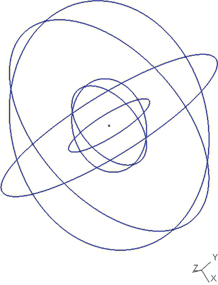
FIGURE 16.3 gmsh concentric spheres prior to meshing.
Figure 16.4 shows the concentric spheres after meshing. A very low-resolution mesh is used for this figure (cl = 1.0). This number will be dropped to cl = 0.1 for actual FEM calculations. This figure shows that the desired geometry has, indeed, been generated; the region between two concentric spheres is meshed.
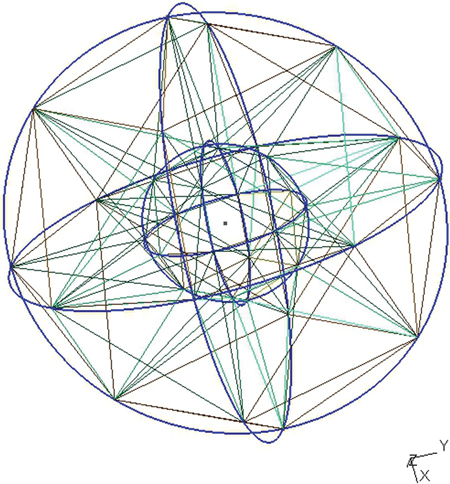
FIGURE 16.4 Concentric spheres after meshing.
16.2 The FEM Coefficient Matrix in Three Dimensions
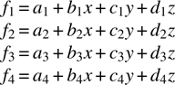
The derivation of the coefficient matrix terms in three dimensions using tetrahedron elements and a four-point function is a direct extension of the derivations of the 2d matrix terms in Chapter 13. We begin by defining the voltage anywhere in the tetrahedron with the function
where f i are the basis functions and (x 1,y 1,z 1), and so on, are the vertices of the tetrahedron:
Then ai , bi ci , and di are determined by the following four sets of conditions:
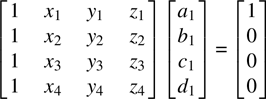

… and so on.
The coefficient matrix in the equations above is related to the volume of the tetrahedron by2

The electric field components are given by
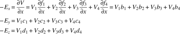
and then

The energy stored in the tetrahedron is

where the integral is over the tetrahedron T and vT is the volume of the tetrahedron given by equation (16.5).
For tetrahedron n with nodes n 1, n 2, n 3, and n 4, the terms that must be added to the coefficient matrix, found by taking the partial derivatives with respect to V 1, V 2 , V 3, and V 4, are
To row n 1, column n 1:
To (n 1, n 2):
To (n 1, n 3):
To (n 1, n 4):
To (n 2, n 1):
To (n 2, n 2):
and so on.
16.3 Parsing the gmsh Files and Setting Boundary Conditions
The file parsing script has been rewritten to handle the 3d mesh; here is the MATLAB script parse_msh_file_3d.m—a 3d gmsh parsing script:
% parse_msh_file_3d.m
% Read the mesh file generated by gmsh and parse it
% This version is for 3d tetrahedron (4 node) structures

%   Element types handled are 1 = line, 2 = 3 node triangle, 15 = point
% 4 = tetrahedron

 filename = uigetfile('*.msh'), % read the file
 fid = fopen(filename, 'r'),

 tline = fgetl(fid); % read the first file line
 if (strcmp(tline, '$MeshFormat')) == 0 % Verify file type
  'Problem with this file'
  nodes_3d = []; tets_3d = []; bcs_3d = [];
  fclose (fid);
  return
 end

 tline = fgetl(fid); % look for version number
 [header] = sscanf(tline, '%f %d %d'),
 if (header(1) ~ = 2.2), 'Possible gmsh version incompatibility', end;
 tline = fgetl(fid); % Look for $EndMeshFormat
 if (strcmp(tline, '$EndMeshFormat')) == 0
  'No $EndMeshFormat Line found'
  nodes_3d = []; tets_3d = []; bcs_3d = [];
  fclose (fid);
  return
 end

 tline = fgetl(fid); % Look for $Nodes
 if (strcmp(tline, '$Nodes')) == 0
  'No $Nodes Line found'
  nodes_3d = []; tets_3d = []; bcs_3d = [];
  fclose (fid);
  return
 end

 nr_nodes = fscanf(fid, '%d', 1); % get number of nodes
 nodes_3d = zeros(nr_nodes, 3); % allocate nodes array
 for i = 1 : nr_nodes % get nodes information
  temp = fscanf(fid, '%g', 4);
  n = temp(1);
  nodes_3d(n,:) = temp(2:4);
 end
 fgetl(fid); % Clear the line

 tline = fgetl(fid); % Look for $EndNodes
 if (strcmp(tline, '$EndNodes')) == 0
  'No $EndNodes Line found'
  nodes = []; tet = []; bcs_3d = {};
  fclose (fid);
  return
 end

 tline = fgetl(fid); % Look for $Elements
 if (strcmp(tline, '$Elements')) == 0
  'No $Elements Line found'
  nodes_3d = []; tets_3d = []; bcs_3d = [];
  fclose (fid);
  return
 end

 tets_3d = []; bcs_3d = [];
 nr_elements = fscanf(fid, '%d', 1); % get number of elements
 for i = 1: nr_elements % process elements information
  temp = fscanf(fid, '%d %d', 2); % get element type
  if temp(2) == 15 | temp(2) == 1 % defined point or line
   fgetl(fid); % clear the (file) line
  elseif temp(2) == 2 % defined triangle
   temp2 = fscanf(fid, '%d %d %d %d %d %d', 6);
   bcs_3d = [bcs_3d; [temp2(3:6)', 88888.8]];
   fgetl(fid);
  elseif temp(2) == 4 % created mesh tetrahedron
   temp3 = fscanf(fid, '%d %d %d %d %d %d %d', 7);
   tets_3d = [tets_3d; temp3(4:7)'];
   fgetl(fid);
  else
   'Unknown type in mesh file'
   nodes_3d = []; tets_3d = []; bcs_3d = [];
   fclose (fid);
   return
  end
 end
 fclose (fid);

 nr_bc_lines = length(bcs_3d);
 'bcs file: '
 bcs_3d
 disp ('Set bcs for all surfaces: '),
 for i = 1 : nr_bc_lines
  if bcs_3d(i,5) == 88888.8 % check for dummy index
   itri = bcs_3d(i,1);
   fprintf ('Surface nr %d :
', itri)
   j = input('Enter bc: ') % decide on the bc
   for k = 1 : nr_bc_lines % set the bc
    if bcs_3d(k,1) == itri, bcs_3d(k,5) = j; end;
   end
   'bcs file: '
   bcs_3d
  end
 end

 filename = input('Name for output files, NO OVERWRITE CHECKING: ', 's'),
 nodes_file_name = strcat('nodes_3d_', filename, '.txt'),
 tets_file_name = strcat('tets_3d_', filename, '.txt'),
 bcs_file_name = strcat('bcs_3d_', filename, '.txt'),
 fid = fopen (nodes_file_name, 'w'),
 fprintf (fid, '%g	%g	%g
', nodes_3d'),
 fclose (fid);
 fid = fopen (tets_file_name, 'w'),
 fprintf (fid, '%d	%d	%d	%d
', tets_3d'),
 fclose (fid);
 fid = fopen (bcs_file_name, 'w'),
 fprintf (fid, '%d	%d	%d	%d	%f
', bcs_3d'),
 fclose (fid);
The logic of this script is the same as in previous versions except that now the bc setting is prompted by defined surfaces rather than by defined lines. This is why the face groupings for the surfaces (in this example, the two spheres) are numbered to clarify the linkage between the faces and their respective volume surfaces. The FEM model will work with any potential difference between the electrodes (spheres in this example), but the capacitance calculation to be described assumes a 1 V potential difference between these electrodes, so it is prudent to use this value if the capacitance calculation is of interest.
The FEM analysis is, as the analysis indicated it would be, a direct extensions of the 2d analysis programs: There is almost nothing to comment on about these programs.
- MATLAB script
fed_3d.m— 3d FEM analysis program:% 3d FEM with triangles % fem_3d.m close all filename = input('Generic name for input files: ', 's'), nodes_file_name = strcat('nodes_3d_', filename, '.txt'), tets_file_name = strcat('tets_3d_', filename, '.txt'), bcs_file_name = strcat('bcs_3d_', filename, '.txt'), % get node data from file dataArray = load(nodes_file_name); nds.x = dataArray(:,1); nds.y = dataArray(:,2); nds.z = dataArray(:,3); nr_nodes = length(nds.x) % get tetrahedrons data from file tets = (load(tets_file_name))'; [tets_width, nr_tets] = size(tets); % get bcs data from file %[bcs_nodes, bcs_volts] = get_bcs_3d(bcs_file_name); dataArray = load(bcs_file_name); bcs_nodes = dataArray(:,2:4); bcs_volts = dataArray(:,5); nr_bcs = length(bcs_volts) % allocate the matrices a = sparse(nr_nodes, nr_nodes); f = zeros(nr_nodes,1); b = zeros(4,1); c = zeros(4,1); d = zeros(4,1); dd = ones(4,4); % generate the matrix terms for tet = 1: nr_tets % Walk through all the triangles n1 = tets(1,tet); n2 = tets(2,tet); n3 = tets(3,tet); n4 = tets(4,tet); dd(1,2) = nds.x(n1); dd(1,3) = nds.y(n1); dd(1,4) = nds.z(n1); dd(2,2) = nds.x(n2); dd(2,3) = nds.y(n2); dd(2,4) = nds.z(n2); dd(3,2) = nds.x(n3); dd(3,3) = nds.y(n3); dd(3,4) = nds.z(n3); dd(4,2) = nds.x(n4); dd(4,3) = nds.y(n4); dd(4,4) = nds.z(n4); vol = det(dd)/6; % volume of the tetrahedron temp = dd[1;0;0;0]; b(1) = temp(2); c(1) = temp(3); d(1) = temp(4); temp = dd[0;1;0;0]; b(2) = temp(2); c(2) = temp(3); d(2) = temp(4); temp = dd[0;0;1;0]; b(3) = temp(2); c(3) = temp(3); d(3) = temp(4); temp = dd[0;0;0;1]; b(4) = temp(2); c(4) = temp(3); d(4) = temp(4); a(n1,n1) = a(n1,n1) + vol*(b(1)^2 + c(1)^2 + d(1)^2); a(n1,n2) = a(n1,n2) + vol*(b(1)*b(2) + c(1)*c(2) + d(1)*d(2)); a(n1,n3) = a(n1,n3) + vol*(b(1)*b(3) + c(1)*c(3) + d(1)*d(3)); a(n1,n4) = a(n1,n4) + vol*(b(1)*b(4) + c(1)*c(4) + d(1)*d(4)); a(n2,n1) = a(n2,n1) + vol*(b(2)*b(1) + c(2)*c(1) + d(2)*d(1)); a(n2,n2) = a(n2,n2) + vol*(b(2)^2 + c(2)^2 + d(2)^2); a(n2,n3) = a(n2,n3) + vol*(b(2)*b(3) + c(2)*c(3) + d(2)*d(3)); a(n2,n4) = a(n2,n4) + vol*(b(2)*b(4) + c(2)*c(4) + d(2)*d(4)); a(n3,n1) = a(n3,n1) + vol*(b(3)*b(1) + c(3)*c(1) + d(3)*d(1)); a(n3,n2) = a(n3,n2) + vol*(b(3)*b(2) + c(3)*c(2) + d(3)*d(2)); a(n3,n3) = a(n3,n3) + vol*(b(3)^2 + c(3)^2 + d(3)^2); a(n3,n4) = a(n3,n4) + vol*(b(3)*b(4) + c(3)*c(4) + d(3)*d(4)); a(n4,n1) = a(n4,n1) + vol*(b(4)*b(1) + c(4)*c(1) + d(4)*d(1)); a(n4,n2) = a(n4,n2) + vol*(b(4)*b(2) + c(4)*c(2) + d(4)*d(2)); a(n4,n3) = a(n4,n3) + vol*(b(4)*b(3) + c(4)*c(3) + d(4)*d(3)); a(n4,n4) = a(n4,n4) + vol*(b(4)^2 + c(4)^2 + d(4)^2); end %bcs for i = 1: nr_bcs if bcs_volts(i) ~ = -9999 % Line 1 of 2 for problem 16.3 for j = 1 : 3 n = bcs_nodes(i,j); a(n,:) = 0; a(n,n) = 1; f(n) = bcs_volts(i); end end % Line 2 of 2 for problem 16.3 end % There might be a few nodes such as a sphere center that are not % connected to anything. We could eliminate them and renumber % or, simpler, just stop them from making trouble: for i = 1 : nr_nodes if a(i,i) == 0 a(i,:) = 0; a(i,i) = 1; end end v = af; % calculate capacitance C = get_tet3d_cap(v, nr_nodes, nr_tets, nds, tets) - MATLAB function
get_tet3d_cap.m:function C = get_tet3d_cap(v, nr_nodes, nr_tets, nds, tets) % Calculate the capacitance of a 3d tetrahedron structure % Simple linear approx. function is assumed eps0 = 8.854; b = zeros(4,1); c = zeros(4,1); d = zeros(4,1); dd = ones(4,4); U = 0; for tet = 1: nr_tets % Walk through all the triangles n1 = tets(1,tet); n2 = tets(2,tet); n3 = tets(3,tet); n4 = tets(4,tet); dd(1,2) = nds.x(n1); dd(1,3) = nds.y(n1); dd(1,4) = nds.z(n1); dd(2,2) = nds.x(n2); dd(2,3) = nds.y(n2); dd(2,4) = nds.z(n2); dd(3,2) = nds.x(n3); dd(3,3) = nds.y(n3); dd(3,4) = nds.z(n3); dd(4,2) = nds.x(n4); dd(4,3) = nds.y(n4); dd(4,4) = nds.z(n4); vol = det(dd)/6; temp = dd[1;0;0;0]; b(1) = temp(2); c(1) = temp(3); d(1) = temp(4); temp = dd[0;1;0;0]; b(2) = temp(2); c(2) = temp(3); d(2) = temp(4); temp = dd[0;0;1;0]; b(3) = temp(2); c(3) = temp(3); d(3) = temp(4); temp = dd[0;0;0;1]; b(4) = temp(2); c(4) = temp(3); d(4) = temp(4); U = U + vol*( (v(n1)*b(1) + v(n2)*b(2) + v(n3)*b(3) + v(n4)*b(4))^2 ... + (v(n1)*c(1) + v(n2)*c(2) + v(n3)*c(3) + v(n4)*c(4))^2 ... + (v(n1)*d(1) + v(n2)*d(2) + v(n3)*d(3) + v(n4)*d(4))^2 ); end U = U*eps0/2; C = 2*U; % Potential difference of 1 volt assumed end
One small addition to the 3d FEM program is the code in lines 73–80 of fed_3d.m. Because of the nature of gmsh, the nodes that define the centers of the circle arcs that ultimately define the spheres show up as defined nodes in the .msh file. These nodes are added into the node count and appear as empty rows in the coefficient matrix (the nodes don't connect to anything, they're just reference points). The program could be written to sniff out these nodes, eliminate them and reduce the node count, but this could complicate the program debugging process because node numbers have been changed from the original gmsh nonde numbers. Instead, the simple task of just making these nodes dummy boundary conditions is performed. Since there are very few of these nodes in a structure description, the overall efficiency of the solution is not diminished meaningfully, and the node numbering is preserved. Also, since these nodes are not part of any tetrahedron, the dummy boundary condition does not contribute to the total energy (capacitance) calculation.
With a gmsh resolution of cl = 0.1, fem_3d.m predicts a capacitance of 137.2 pF. The exact capacitance may be calculated from basic principles, namely

so that
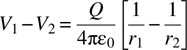
Figure 16.5 shows the FEM predicted voltage distribution between the spheres (tickmarks ×) overlaid on the exact solution (continuous line).

FIGURE 16.5 Voltage distribution between the spheres.
16.4 Open Boundaries and Cylinders in Space
// struct16_4 2 Cylinders

// geometry
cl = .5;
rc = 1.; // cylinder radius
rs = 7.; // sphere radius
xs = 3; // cylinder center-center separation
zs = 4; // cylinder height

// First cylinder ------------------------------------

Point(1) = {-xs/2, 0, -zs/2, cl}; // center of first circle
Point(2) = {-xs/2 + rc, 0, -zs/2, cl};
Point(3) = {-xs/2, rc, -zs/2, cl};
Point(4) = {-xs/2-rc, 0, -zs/2, cl};
Point(5) = {-xs/2, -rc, -zs/2, cl};

Circle(1) = {2, 1, 3}; // 1/4 circle segments
Circle(2) = {3, 1, 4};
Circle(3) = {4, 1, 5};
Circle(4) = {5, 1, 2};

Line Loop(1) = {1, 2, 3, 4}; // bottom of cylinder
Plane Surface(1) = {1};

Point(6) = {-xs/2, 0, zs/2, cl}; // center of second circle
Point(7) = {-xs/2 + rc, 0, zs/2, cl};
Point(8) = {-xs/2, rc, zs/2, cl};
Point(9) = {-xs/2-rc, 0, zs/2, cl};
Point(10) = {-xs/2, -rc, zs/2, cl};

Circle(5) = {7, 6, 8}; // 1/4 circle segments
Circle(6) = {8, 6, 9};
Circle(7) = {9, 6, 10};
Circle(8) = {10, 6, 7};

Line Loop(2) = {5, 6, 7, 8};
Plane Surface(2) = {2};

Line(10) = {2, 7}; // connecting lines for cylinder walls
Line(11) = {3, 8};
Line(12) = {4, 9};
Line(13) = {5, 10};

Line Loop(3) = {5, -11, -1, 10};
Line Loop(4) = {6, -12, -2, 11};
Line Loop(5) = {7, -13, -3, 12};
Line Loop(6) = {8, -10, -4, 13};

Ruled Surface(3) = {3};
Ruled Surface(4) = {4};
Ruled Surface(5) = {5};
Ruled Surface(6) = {6};

// Cylinder Surface
Surface Loop(1) = {1, 2, 3, 4, 5, 6};

// Second Cylinder --------------------------------
Point(21) = {xs/2, 0, -zs/2, cl}; // center of second circle
Point(22) = {xs/2 + rc, 0, -zs/2, cl};
Point(23) = {xs/2, rc, -zs/2, cl};
Point(24) = {xs/2-rc, 0, -zs/2, cl};
Point(25) = {xs/2, -rc, -zs/2, cl};

Circle(21) = {22, 21, 23}; // 1/4 circle segments
Circle(22) = {23, 21, 24};
Circle(23) = {24, 21, 25};
Circle(24) = {25, 21, 22};

Line Loop(21) = {21, 22, 23, 24}; // bottom of cylinder
Plane Surface(21) = {21};

Point(26) = {xs/2, 0, zs/2, cl}; // center of second circle
Point(27) = {xs/2 + rc, 0, zs/2, cl};
Point(28) = {xs/2, rc, zs/2, cl};
Point(29) = {xs/2-rc, 0, zs/2, cl};
Point(30) = {xs/2, -rc, zs/2, cl};

Circle(25) = {27, 26, 28}; // 1/4 circle segments
Circle(26) = {28, 26, 29};
Circle(27) = {29, 26, 30};
Circle(28) = {30, 26, 27};

Line Loop(22) = {25, 26, 27, 28};
Plane Surface(22) = {22};

Line(30) = {22, 27}; // connecting lines for cylinder walls
Line(31) = {23, 28};
Line(32) = {24, 29};
Line(33) = {25, 30};

Line Loop(23) = {25, -31, -21, 30};
Line Loop(24) = {26, -32, -22, 31};
Line Loop(25) = {27, -33, -23, 32};
Line Loop(26) = {28, -30, -24, 33};

Ruled Surface(23) = {23};
Ruled Surface(24) = {24};
Ruled Surface(25) = {25};
Ruled Surface(26) = {26};

// Cylinder Surface
Surface Loop(21) = {21, 22, 23, 24, 25, 26};

// Outer sphere --------------------------------------------

// points
Point(41) = {0, 0, 0, cl}; // center
Point(42) = {0, 0, rs, cl};
Point(43) = {-rs, 0, 0, cl};
Point(44) = {0, 0, -rs, cl};
Point(45) = {rs, 0, 0, cl};
Point(46) = {0, -rs, 0, cl};
Point(47) = {0, rs, 0, cl};

// 1/4 circle segments
Circle(41) = {42, 41, 43};
Circle(42) = {43, 41, 44};
Circle(43) = {44, 41, 45};
Circle(44) = {45, 41, 42};
Circle(45) = {43, 41, 46};
Circle(46) = {46, 41, 45};
Circle(47) = {45, 41, 47};
Circle(48) = {47, 41, 43};
Circle(49) = {42, 41, 46};
Circle(50) = {46, 41, 44};
Circle(51) = {44, 41, 47};
Circle(52) = {47, 41, 42};

// 1/8 sphere surface outlines
Line Loop(41) = {41, 45, -49};
Line Loop(42) = {44, 49, 46};
Line Loop(43) = {42, -50, -45};
Line Loop(44) = {43, -46, 50};
Line Loop(45) = {41, -48, 52};
Line Loop(46) = {44,-52, -47};
Line Loop(47) = {42, 51, 48};
Line Loop(48) = {43, 47, -51};

// 1/8 sphere ruled surface
Ruled Surface(41) = {41};
Ruled Surface(42) = {42};
Ruled Surface(43) = {43};
Ruled Surface(44) = {44};
Ruled Surface(45) = {45};
Ruled Surface(46) = {46};
Ruled Surface(47) = {47};
Ruled Surface(48) = {48};

// Sphere surface
Surface Loop(41) = {41, 42, 43, 44, 45, 46, 47, 48};

// build the volume

// Volume(1) = {1};
// Volume(21) = {21};
Volume(41) = {41, 1, 21};
The gmsh script struct16_4.geo shows the construction of two cylinders and a surrounding sphere. The cylinders are constructed in the same manner as the spheres; ruled surfaces of a ![]() cylinder are constructed, circles for the top and bottom of the cylinder are constructed, and then they are all joined together as a surface loop. The final volume command establishes the region to be meshed as the insider of the sphere absent the two cylinders.
cylinder are constructed, circles for the top and bottom of the cylinder are constructed, and then they are all joined together as a surface loop. The final volume command establishes the region to be meshed as the insider of the sphere absent the two cylinders.
The wire frame model for all of this, when the outer sphere radius is 4.0, is shown in Figure 16.6.
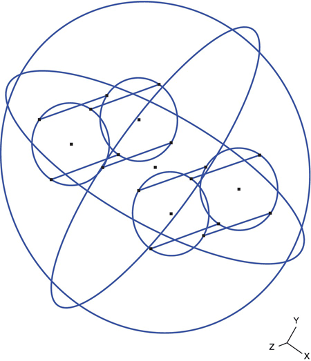
FIGURE 16.6 Wire frame model for two cylinders in a sphere.
The capacitance between the two cylinders, in an unbounded region, is approximated by setting the cylinder potentials to +0.5 and -0.5, setting the outer-sphere potential to 0, and increasing the sphere radius until the sphere no longer contributes to the capacitance. Increasing the sphere radius by adding lower and lower resolution shells, as described in Chapter 15, is an approach that takes more time to set up but ultimately makes better use of computer resources.
Problems
- 16.1 Create a
gmshfile for Figure P16.1. Run the FEM analysis and calculate the capactiance of the structure. - 16.2 We can model a small screw as a metallic right cylinder. Modify the structure of
structp16_1.geoby adding such a cylinder, of radius 0.25 cm, to the center of the top of the box. Calculate the capacitance as a function of the depth that this screw reaches into the box. - 16.3
structp16_1.geohas symmetry planes X = 0 and Y = 0. Z = 0 looks a bit like a symmetry plane, but it is not a symmetry plane because the strip conductor is not centered in Z in the box. Write a new version ofstructp16_1.geoshowing only one-fourth of the structure to utilize these symmetries. Rewrite whichever MATLAB programs are necessary to perform the calculations on this data file. - 16.4 The goals of this problem and Problem 16.5 are to add dielectric material capability to the 3d FEM analysis. The first task is to modify
fem_3d.mto properly handle individual tetrahedron dielectric constants. Rather than “patching” the dielectric region definition into the FEM program as was done with the 2d analysis, modify the file structure so that the dielectric information is part of the tetrahedron data file. A separate small program will then be necessary to supply the correct dielectric information to the file. - 16.5 Improve the dielectric calculation accuracy of Problem 16.4.
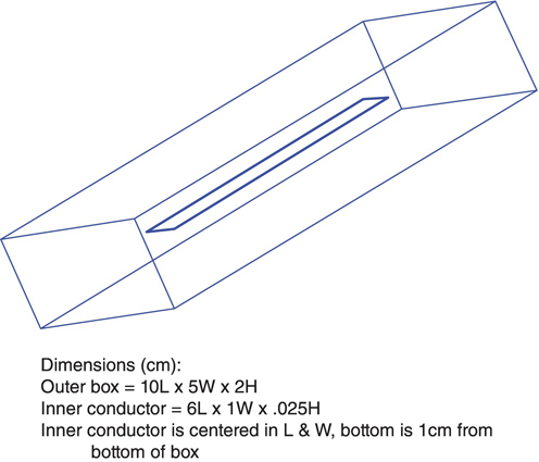
FIGURE P16.1 Structure and dimensions for Problem 16.1.
References
- 1. P. Knupp and S. Steinberg, Fundamentals of Grid Generation. CRC Press, Boca Raton, FL, 1994.
- 2.
http://mathworld.wolfram.com/Tetrahedron.html.