
1
A Review of Basic Electrostatics
Electric and magnetic phenomena, including electromagnetic wave propagation, are described by Maxwell’s equations.1 When nothing is changing with time, that is, when all derivatives with respect to time are zero, the electric and the magnetic phenomena decouple and become separate electric and magnetic phenomena. These are referred to respectively as electrostatics, which describes the properties of systems with separated static regions of positive and negative electric charge (although the entire system is charge-neutral), and magnetostatics, which describes the properties of systems with electric currents and/or magnetized materials.
In this book we shall consider only electrostatics. This subset of a subset of topics describes a vast number of real-world situations. Chapter 2 describes some practical needs and uses of electrostatic analyses, the remainder of the book will be dedicated to examining several techniques for performing these analyses.
The materials to follow are intended to be a quick review of the relationships that will be used throughout this book. The intent here is to provide a consistent set of notation using all the relationships that will be needed going forward. Many of these relationships are stated without derivation or proof. A more complete electrostatics theory text is recommended for newcomers to the subject. There are very many excellent texts available. The references list at the end of this chapter is certainly not exhaustive, but the texts cited are considered standards in the field.
1.1 Charge, Force, and the Electric Field
Electric charges exert forces on one another. This is the basis of electrostatics. The characteristics of these forces are summarized in Coulomb’s law:
- Electric charge carries a polarity, or sign. The choice of sign was originally arbitrary, but now is established by tradition—the electron, the most common charged subatomic particle, carries a negative charge.
- For point charges q1 and q2, measured in coulombs, the (coulomb) force, measured in newtons, in a uniform medium, is given by
(1.1)

- In equation (1.1) and elsewhere ε is the permittivity of the material in farads per meter (F/m). In free space, ε = ε0 = 8.854 F/m. For other linear, isotropic, homogeneous materials, ε = kε0, where k is the relative permittivity, the relative dielectric constant, or sometimes simply the dielectric constant, of the material. Farads per se are defined as coulombs per volt (C/V). In this book we shall consider only linear, isotropic, homogeneous dielectric materials, and going forward this will be assumed.
- In equation (1.1) r is the distance between q 1 and q 2.
- Also,
 is a unit vector along the line connecting q
1 and q
2. If q
1 and q
2 have the same sign, then
is a unit vector along the line connecting q
1 and q
2. If q
1 and q
2 have the same sign, then  is pushing q
1 and q
2 apart. If q
1 and q
2 have opposite signs,
is pushing q
1 and q
2 apart. If q
1 and q
2 have opposite signs,  is pulling them together.
Equation (1.1) is expressed in the rationalized meter-kilogram-second (mks) system of units. The derivation of this set of units is an interesting discussion in itself.2
When a test charge is in the area of a collection of charges and the magnitude of these latter charges is sufficient, relative to the test charge, to render negligible any perturbation of the situation due to the test charge, then the force on the test charge divided by its charge is defined to be the electric field at that point (typically called the field point). The electric field at (the field point) p due to a charge q is therefore

where ![]() is the unit vector along the line from charge q to point p and r is the distance from charge q to point p. The values of
is the unit vector along the line from charge q to point p and r is the distance from charge q to point p. The values of ![]() are expressed in volts per meter (V/m).
are expressed in volts per meter (V/m).
Since the test charge at p in the preceding example doesn’t disturb the electric field, the electric field is considered to be a consequence of q; in other words, the test charge doesn’t have to be present for the field to exist.
The term ![]() is a vector with both magnitude and direction. The direction of
is a vector with both magnitude and direction. The direction of ![]() anywhere in space is identically the direction of the force that would be experienced by a (positive) test charge at that point. We can look at the field lines of
anywhere in space is identically the direction of the force that would be experienced by a (positive) test charge at that point. We can look at the field lines of ![]() as a representative of the direction of the force on a test charge due to q. For a single-point charge, the field lines are simply radial lines pointing away from the charge. The lines point away because a positive test charge placed anywhere would feel a force pushing it away from the (source) charge. The magnitude of the field decreases with the square of the distance from the charge.
as a representative of the direction of the force on a test charge due to q. For a single-point charge, the field lines are simply radial lines pointing away from the charge. The lines point away because a positive test charge placed anywhere would feel a force pushing it away from the (source) charge. The magnitude of the field decreases with the square of the distance from the charge.
For a collection of charges, the electric field at any point is the sum of the contributions of all of the charges in the collection. Figure 1.1, for example, shows electric field lines in the X–Y plane for two point charges placed at (-1,0,0) and (+1,0,0). In part (a) the two charges are identical; in part (b) they are the same in magnitude but opposite in sign.
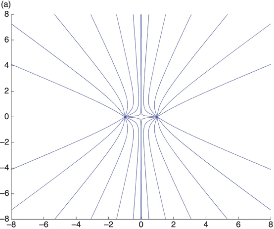
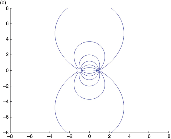
FIGURE 1.1 Electric field lines for point charges at (-1,0,0) and (1,0,0).
In order to calculate ![]() directly we must keep track of the vector components of every charge contributing to it. Continuing with the example of Figure 1.1, the simple MATLAB function
directly we must keep track of the vector components of every charge contributing to it. Continuing with the example of Figure 1.1, the simple MATLAB function charges.m shown here calculates the field anywhere in the X–Y plane. Calculation of the field components from the geometry is shown in the equations in this program. Setting q
2 to +1 or -1 produces the two cases discussed above.
function [ Ex, Ey, Emag ] = charges(x,y)
% This function calculates the electric field for the 2 charge
% layout of Figure 1.1

q2 = -1;    % Set this to +1 or -1 as needed
eps = 8.854;  % pFd/m in free space
theta1 = atan2(y,x + 1);     theta2 = atan2(y,x-1);
rsq1 = (x + 1).^2 + y.^2;     rsq2 = (x-1).^2 + y.^2
Emag1 = 1./(4*pi*eps*rsq1);   Emag2 = 1./(4*pi*eps*rsq2);
Ex1 = Emag1.*cos(theta1);     Ex2 = q2*Emag2.*cos(theta2);
Ey1 = Emag1.*sin(theta1);     Ey2 = q2*Emag2.*sin(theta2);


Ex = Ex1 + Ex2;   Ey = Ey1 + Ey2;
Emag = sqrt(Ex.^2 + Ey.^2);


end
If both charges are equal to +1 in this example, then along the y axis Ex must always be zero. This can be deduced from the symmetry of the situation without consulting the equations. On the other hand Ey is zero only at y = 0 and must be an odd function of y. Ey (0,y,0) is shown in Figure 1.2.
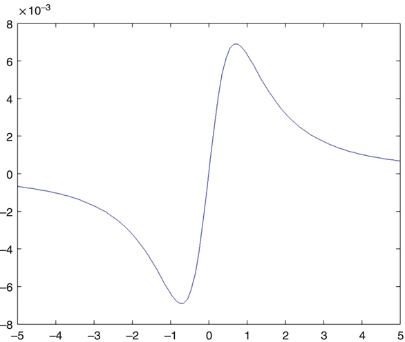
FIGURE 1.2 Ey (0,y,0) for two identical positive charges.
If the right-hand charge (in Figure 1.2) is changed to -1, then, along the y axis Ey must always be zero—again, from symmetry considerations. Ex in this case is an even positive function of y, as shown in Figure 1.3.
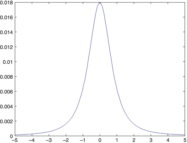
FIGURE 1.3 Ex (0,y,0) for two charges of opposite sign.
If a small charged mass such as an electron is placed near charge(s), as in part (a) or (b) of Figure 1.1, it would immediately start moving. Its trajectory would not be along a field line. Since the electron has mass, it gathers momentum as it moves and a proper description of its motion requires solving Newton’s equation with the electric field as the driving force. Electron trajectories in various electric field profiles will be examined in Chapter 17.
Inspection of Figure 1.1a shows that the field lines emanating from both charges start out radially. They then bend rather than cross and leave the region, going instead to infinity. This characteristic is identical to the radial field lines from a single charge which also go to infinity. In Figure 1.1b, however, each field line travels from the positive (left-hand) charge to the negative (right-hand) charge and terminates. This is characteristic of an electrically neutral structure, and we can extract a general rule: Electric field lines originate at and terminate at charge; a neutral structure will have no field lines going to infinity. This will be expressed as a mathematical relationship in Section 1.2.
1.2 Electric Flux Density and Gauss’s Law
Let us define a (vector) quantity ![]() as follows:
as follows:
Combining this definition with equation (1.2), we obtain
which is independent of the dielectric constant.
The ![]() in these equations is the electric flux density. The rationale for using this term will become clear shortly. Consider a point charge q surrounded by a virtual spherical shell of radius r
0. The surface area of this shell is
in these equations is the electric flux density. The rationale for using this term will become clear shortly. Consider a point charge q surrounded by a virtual spherical shell of radius r
0. The surface area of this shell is ![]() . Since
. Since ![]() is a function only of r, it is a constant everywhere on this shell; also, since it is pointed radially outward everywhere, it is normal to the shell at intersection. The integral of (the magnitude of)
is a function only of r, it is a constant everywhere on this shell; also, since it is pointed radially outward everywhere, it is normal to the shell at intersection. The integral of (the magnitude of) ![]() over the surface of the shell is
over the surface of the shell is

By examining the situation for an arbitrary collection of charges and an arbitrary surface surrounding them, we can generalize this result to Gauss’s law3

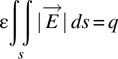
where the integral is over the entire surface. ![]() is a differential area with vector direction normal to the plane of the area and q is the total charge enclosed.
is a differential area with vector direction normal to the plane of the area and q is the total charge enclosed.
Returning to equation (1.5), we have
For a spherical shell centered at q, we obtain ![]() only, pointing radially outward, and therefore
only, pointing radially outward, and therefore
which is essentially identical to equation (1.2). In other words, Gauss’s and Coulomb’s laws are equivalent.
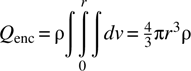
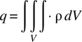
Suppose that we have a sphere of charge of radius a, centered at the origin, of uniform charge density ρ [expressed in coulombs per cubic meter (C/m3)] (see Figure 1.4).
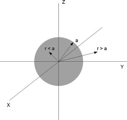
FIGURE 1.4 Sphere of uniform charge density ρ.
From the symmetry of the situation, we know again that ![]() only, pointing radially outward. For any r ≤ a, the charge enclosed is
only, pointing radially outward. For any r ≤ a, the charge enclosed is
Putting this result into Gauss’s law, we have
or
The field goes to 0 at r = 0, because there is no charge enclosed. It increases with increasing r. At r = a all of the charge is enclosed and again using Gauss’ law, for r ≥ a, we obtain
and then
If ρ is not a constant but is instead a function of r (and only r), then it must be brought inside the integral of equation (1.9) and the integral properly evaluated. The electric field outside the sphere of charge (r ≥ a) depends only on the total charge in the sphere, irrespective of the details of ρ(r). This latter point is significant because it tells us that E(r) (see Figure 1.5) will be the same (again, for r ≥ a), if all the charge is concentrated at a point at the origin, is spread uniformly through the volume of the sphere, or is distributed in whatever other configuration that can be imagined. An important case we will consider (in Section 1.3) is the case where all of the charge resides in a thin shell at r = a.
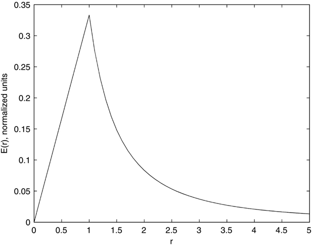
FIGURE 1.5 E(r) for a sphere of radius a, charge density ρ.
1.3 Conductors
An ideal conductor of charge is a material in which the charge carriers are free to move about under the influence of electrostatic forces (Coulomb’s law). Good examples of this are metals such as copper and silver—they are not ideal conductors but they are very good conductors. The very mobile charge in metals is the electrons in the outer shell of the metallic atoms; how charge mobility comes about is an important topic of solid-state physics.4 How charge is arranged in conductors in different situations will be a central theme in discussion of the method of moments (MoM) in later chapters (Chapters 3, 4, etc.). Right now we will consider only situations with geometries whose symmetries require that charge distributions be uniform.
Consider Figure 1.6. A metal sphere has been placed at r = a, and a spherical metal shell has been placed at r = b. A charge -Q equal to the total charge enclosed by the inner shell (+Q) has been placed on the outer shell so that the entire system is now charge-neutral. The symmetry of the structure implies that charge must be uniform in terms of angle. The charges on the inner sphere repel each other and are attracted to the charges on the outer sphere. This means that the charges on the inner sphere will all move to the outer surface of the inner sphere, which, in turn, means that there is no electric field inside the inner sphere. A further conclusion is that, in terms of the electric field between the outer shell and the inner sphere, the inner sphere can be either a solid conductor or simply a thin conductor shell at r = a.
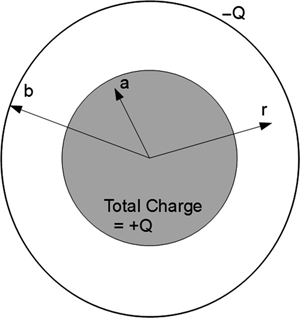
FIGURE 1.6 Two concentric spherical shells.
This latter characteristic of electrostatic systems is put to very good use in ultra-high-voltage systems such as the Van de Graaff generator.5 The safest place for people to be is inside one of the large metal spheres used in the device, as it is a field-free region.
Returning to Figure 1.6, in the region a ≤ r ≤ b, charge +Q is enclosed, and
When r ≥ b, the sum of the charge on both the inner shell and the outer shell is zero, so that there is no net charge enclosed and E abruptly drops to zero (Figure 1.7). Next, consider the structure shown in Figure 1.8. Two large parallel conductor plates have surface charge densities +σ and -σ [expressed in coulombs per square meter (C/m2)]. The plates are separated by a distance d.
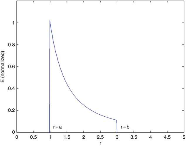
FIGURE 1.7 Electric field between two concentric opposite-charge conductive shells.
Near the center of these plates, far from the edges, the charge density on both plates is uniform. The only possible electric field distribution in this region is uniform, directed from the positively charged plate toward the negatively charged plate. The figure shows a virtual right circular cylinder extending from the bottom plate up to some point between the plates. The actual shape of the virtual structure is insignificant as long as its walls are directed normal to the plates’ surfaces (i.e., parallel to the electric field lines).
If the area of the top and bottom surfaces of the virtual structure is A, the charge enclosed by the structure, as long as the top surface is somewhere between the surfaces, is σA. Because the sidewalls of the structure are parallel to the electric field lines, no lines cross the surfaces, and therefore the only contribution to the right-handside of equation (1.6) is the top surface. Thus Gauss’s law tells us that
or
Gauss’s law can also be expressed in differential, or point, form as3
where ∇ ⋅ is the divergence operator. In rectangular coordinates this is
where ρ = ρ(x,y,z) is the charge density, that is
where V is the total volume enclosed by s.
1.4 Potential, Gradient, and Capacitance
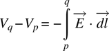
Since there is a force on a charged body in an electric field, moving that body through the field must require work. (If energy is transferred to the body, we’ll consider it negative work done.) This is analogous to the work done lifting a mass in a gravitational field. As in the case of work done in a gravitational field, we can define a potential difference as the work done in moving the body, where ![]() is a differential length element along the path from p to q:
is a differential length element along the path from p to q:

The electrical potential ϕ is also called the voltage V, so equation (1.20) can equivalently be written
As the preceding equations show, only a voltage difference between two points is defined. Strictly speaking, the voltage at a point has no meaning. It is common, however, to define the voltage at some point as zero, often called the ground or reference voltage or potential. It is then possible to refer to the voltage at any point using a single number—the implied meaning is that we are talking about the voltage difference between that point and the reference point.
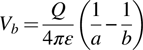
Returning to the example of the concentric spheres (Figure 1.6), we can easily find the voltage difference (commonly called the voltage) between the two spheres by integrating equation (1.14):

Here, we have chosen V(a) = 0 as the voltage reference.
The voltage between the two metal shells is then
From a circuital perspective, we are often more interested in voltages (and fields) at different places in terms of the applied voltage. We obtain this result by dividing equation (1.22) by equation (1.23):
For the parallel plate structure (Figure 1.8), taking z = 0 as the bottom plate and z = d as the top plate, with the bottom plate at ground and the top plate at V 0, integrating equation (1.16), and repeating the same procedure as above, we obtain
Again analogous to the mass in a gravitational field, the potential difference between two points is path independent, it is inconsequential which path the integral takes from point p to point q. This implies that the electrostatic field is conservative—any path leading from point p back to point p will yield a zero-voltage difference. In other words, electrostatic energy is neither gained nor lost going around a closed path. An important point to make here, even though it is beyond the purview of this book, is that this is not a general electromagnetic system property—it is valid only in the electrostatic case.
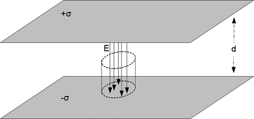
FIGURE 1.8 Electric field between two large parallel plates, near the center.
Restating equation (1.21) to yield the field in terms of the voltage difference, in rectangular coordinates, we have

The operator ∇ is called the gradient operator. This equation shows clearly why an arbitrary reference voltage choice has no effect on the electric field.
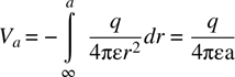
Suppose that there is a charge q at the origin of our coordinate system. If q is the only charge present, then no work was required to bring q from anywhere else to the origin. Now, let us bring a test charge from infinity (where the field due to q is zero) to some radius a. Using equation (1.21), we obtain

and using equation (1.2), the potential at a is
Equation (1.28) is a scalar equation, which is almost always easier to work with than is a vector equation. Also, once the voltage is known, it is a straightforward job to calculate the field. Consequently, we will concentrate on finding voltages and then (if necessary) finding the field, not the other way around.
For the single-point charge of equation (1.28), we already know that the field lines point radially outward (from the charge), going to infinity. Figure 1.9. shows surfaces of constant potential, known as equipotential surfaces or more commonly equipotentials. These surfaces cross the field lines normally and in this situation are spheres.
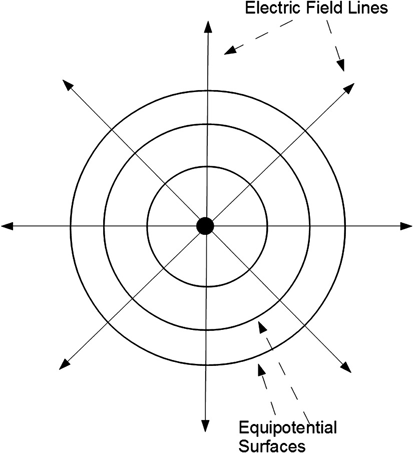
FIGURE 1.9 Electric field lines and equipotential surfaces about a point charge.
If, instead of a single charge q, we have a collection of (discrete) charges, we must replace equation (1.28) by the sum of the contributions of all the charges, and a is replaced by the distances from each of the charges (xi ,yi ,zi ) to the measurement point p = (xp ,yp ,zp ). In other words,
and then
The gradient [equation (1.26)] operating on V produces en electric field vector whose direction is the same as that of the maximum change in V. Since the direction of maximum change from an equipotential contour is always normal to the contour, the electric field lines will always be normal to the equipotential contours. Figure 1.10 is essentially a repeat of Figure 1.1, which shows the electric field lines and the equipotential surfaces about a two-charge system.
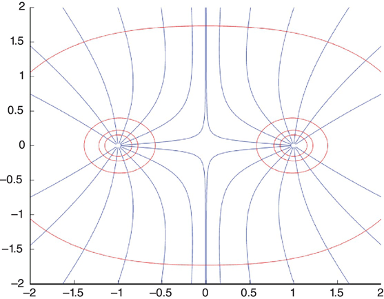
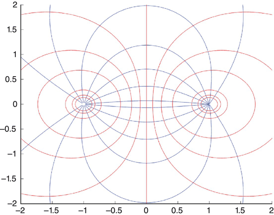
FIGURE 1.10 Repeat of Figure 1.1 with equipotential lines superimposed.
The MATLAB program linesofforce.m generates the curves shown in Figure 1.10 (and Figure 1.1):
% lines of force.m

%  The lines of force between two equal charge
%  q2 may be switched between +1 and -1

close

[x,y] = meshgrid ( -10:.01:10, -10:.01:10 );

q1 = 1; q2 = -1;

theta1 = atan2(y,x + 1);   theta2 = atan2(y,x - 1);
r1sq = (x + 1).^2 + y.^2;   r2sq = (x - 1).^2 + y.^2;

E1x = q1*cos(theta1)./r1sq;  E1y = q1* sin(theta1)./r1sq;
E2x = q2*cos(theta2)./r2sq;  E2y = q2*sin(theta2)./r2sq;

Ex = E1x + E2x;   Ey = E1y + E2y;
startx = [];   starty = [];

for theta = .10: pi/8: .85*pi
 startx = [startx, -1 + .03*cos(theta)];
 starty = [starty, .03*sin(theta)];
end

xy = stream2 ( x, y, Ex, Ey, startx, starty );
figure (1)
axis ([-2, 2, -2, 2])
streamline ( xy );
hold on

xy = stream2 ( x, y, Ex, Ey, startx, -starty );   % symmetry
streamline ( xy );

if q2 >0
 xy = stream2 ( x, y, Ex, Ey, -startx, starty );
 streamline ( xy );

 xy = stream2 ( x, y, Ex, Ey, -startx, -starty );
 streamline ( xy );
end

r1 = sqrt(r1sq); r2 = sqrt(r2sq);

V = (q1./r1 + q2./r2);

V_lines = [[-7:2:7],[-.5,.5, -.2, .2, 0]];
contour (x, y, V, V_lines)
For a distribution of charge with density ρ(xi ,yi ,zi ), we have
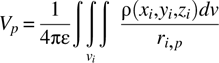
where the integral is over the volume containing the charge distribution.
If we connect a battery between two electrodes, the electrodes assume the potential difference ( i.e., the voltage) of the battery. In this process, some electrons leave the electrode that is connected to the positive terminal of the battery and flow into the battery; an equal number of electrons leave the negative terminal of the battery and flow into its connected electrode. If we were to then remove the battery, this charge imbalance and the voltage difference would remain at the electrodes. The electrode that lost electrons is now positively charged at some charge q, and the electrode that gained electrons is now negatively charged at -q. Both the electrode system (the two electrodes) and the battery remain electrically neutral. Some work has been done in charging the capacitor, and electrochemical changes in the battery that supplied the energy to do this have resulted in some discharging of the battery.
The ratio of the charge q to the voltage difference between the electrodes is called the capacitance of the structure, measured in farads:
For the concentric spherical shells of Figure 1.6, directly from equation (1.23), we obtain
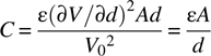
For the central region of a large parallel plate structure (capacitor), we must consider capacitance per unit area. From equation (1.25), we obtain
Equation (1.34) is most often written as the total capacitance for an electrode area A:
Equation (1.35) is known as the ideal parallel plate capacitor relationship. We will see how closely it approximates the capacitance of a real parallel plate capacitor in one of the first examples of calculations using the method of moments, presented later in the book.
1.5 Energy in the Electric Field
Using equation (1.2), the work expended moving a test charge q in the electric field of a capacitor is
If an incremental extra charge dq were then added, the incremental work would be
The work expended in bringing up a total charge Q is
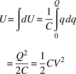
where V is the voltage difference between the capacitor electrodes, that is, the voltage difference to which the capacitor is charged.
In the simple case of an ideal parallel plate capacitor, the electric field is a constant and
The energy density is then
Although this relationship has been derived only for the special case of the ideal parallel plate capacitor, with the help of some vector relationships it can be shown to be true in general.3 This general relationship, for ![]() is then
is then
where the integral is over all space.
Setting equations (1.38) and (1.41), two expressions for the total energy stored in the electric field, equal to each other and bringing in equation (1.26) to express the electric field in terms of the voltage between two electrodes
gives us a way to find the capacitance of a structure without ever explicitly worrying about the charge on the electrodes or the electric field:
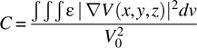
The notation in this equation deserves some clarification: V 0 is the applied voltage at one electrode referred to another electrode of a structure. V(x,y,z) is the voltage distribution throughout the volume (possibly all space) where the electric field is nonzero due to V 0.
Finding the capacitance directly from the voltage distribution will be shown to be a very useful technique when dealing with finite difference or finite element solutions for the voltage distribution.
For an ideal parallel plate capacitor, starting with equation (1.41), we obtain
where 0 ≤ z ≤ d, V 0 is the applied voltage, and the area of the plates is A. Continuing, we obtain

and finally
which, of course, agrees with equation (1.35).
For the concentric spheres, from equation (1.24), we have
so that
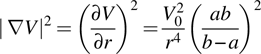
and then, as expected, we obtain

These examples of finding capacitance using the stored energy might seem pointless—the voltage distributions were found from solutions for the electric field in terms of the charge; these distributions were used to find the stored energy and then to find the capacitance “without referring to the field or the charge.” Section 1.6 should clarify this issue. The voltage will be found directly from the structure description, without first looking at the field or the charge.
1.6 Poisson’s and Laplace’s Equations
Combining equations (1.17) and (1.26), again in rectangular coordinates, we have
The operator ∇ ⋅ ∇, written ∇2, is called the Laplacian, and in rectangular coordinates this equation becomes
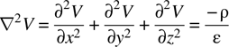
This is Poisson’s equation.
In a charge-free region, Poisson’s equation becomes Laplace’s equation:
Laplace’s equation will prove to be a workhorse throughout much of this book, so it is useful to write out the Laplacian in cylindrical and spherical coordinates. In cylindrical coordinates, we obtain
and in spherical coordinates, looking only at systems with spherical (φ and θ) symmetry, we get
Laplace’s equation, at first blush, seems irrelevant. If there is no charge, what is there to calculate? In many situations, however, we have a structure with two (or more) charged electrodes in an otherwise charge-free region. Consider, for example, two concentric metal shells. While we may never examine the charge explicitly, we can still solve Laplace’s equation for thevoltage distribution in the charge-free region between these shells using the shells as boundary conditions. From equation (1.54), we have
which integrates to
where K 1 is a constant of integration. This, in turn, integrates to
where K 2 is a second constant of integration.
Fortunately, we have two boundary conditions to satisfy: V(a) = 0 and V(b) = V 0. Substituting these conditions into equation (1.57) gives us two equations in the two unknown constants. Solving for these constants and putting the results back into equation (1.57) gives us identically equation (1.47).
In Chapter 2 we will see that in many practical situations a structure is very long and uniform in one dimension and that therefore a cross section of the structure gives us excellent results for V, E, U, and C, the latter two on a per-unit-length basis.
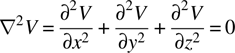
An example of such a structure is the circular coaxial cable shown in Figure 1.11. This is an example of a transmission line; transmission lines will be discussed in Chapter 2. The salient point here is that these are two concentric circular conductors of radii a < b. As long as we are not near the ends of the cylinders, the electrostatic problem is essentially a two-dimensional problem.
FIGURE 1.11 Circular coaxial transmission line and a cross section of the line.
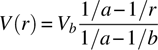
Laplace’s equation in cylindrical coordinates with both circular symmetry and no length (z) dependence is as follows, from equation (1.53):
Again, integrating twice and using the boundary conditions V(a) = 0 and V(b) = V 0, we get

and evaluating equation (1.43):
1.7 Dielectric Interfaces
When a space is uniformly filled with a dielectric material, solution procedures are straightforward. All the conditions and principles discussed and presented above still apply, except for the number actually used for ε. The circular coaxial cable, for example, is often manufactured using a flexible plastic dielectric with a (relative) dielectric constant of approximately 2 separating the inner and outer conductors. In equation (1.60), then, ε = 2ε0, and the analysis is complete.
This is not the case, however, when there are multiple dielectrics, that is, there are dielectric interfaces, present in a structure. Figure 1.12 shows three examples of dielectric interfaces.
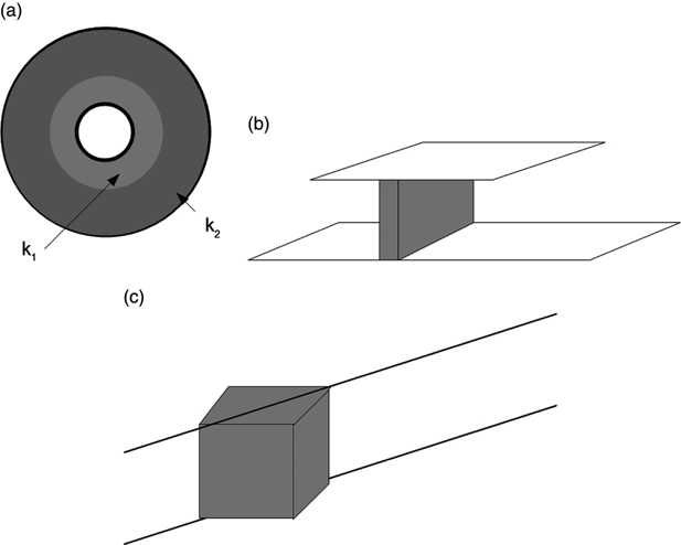
FIGURE 1.12 Three examples of dielectric interfaces.
Figure 1.12a shows the cross section of a coaxial cable with two concentric different dielectric materials between the two electrodes. Figure 1.12b shows a three-dimensional parallel plate capacitor with a slab of dielectric material separating the electrodes. Figure 1.12c shows a block of dielectric material being used as a standoff insulator to separate two power carrying lines. In the latter two cases the dielectric interface is between the dielectric material and the surrounding air.
In Figure 1.12a the direction of the electric field is known — symmetry dictates that it be radial. In Figure 1.12b,c the electric field direction is not known a priori; both the field strength and direction are unknown functions of position and must be found.
Dielectric material regions influence electrostatic solutions in two ways: their dielectric constant itself and the perturbation of the voltage and field distributions in a structure due to the dielectric interfaces. The dielectric interfaces are characterized by boundary conditions that arise at these interfaces.
Consider Figure 1.13a. Shown in cross section, a small virtual pillbox sits between two different dielectric materials. The top and bottom surfaces of the pillbox are of area A. The actual shape of these surfaces doesn’t matter; it could be square, round, or in another configuration. The thickness of the pillbox is Δz. The normal D field components to the top and bottom surfaces is shown.

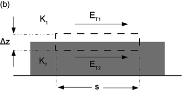
FIGURE 1.13 Boundary between two different dielectric materials.
In the limit as Δz goes to zero (shrinking from the top and bottom toward the middle), contribution to the Gaussian surface whose shape is the pillbox from the sides vanishes, and since there is no charge inside the pillbox, we obtain
or
Now consider Figure 1.13b. In this case the dashed-line rectangle is a two-dimensional path. The integral of the tangential electric field around the path must be zero (the electric field is conservative) so that, as Δz goes to zero, either
or
Equations (1.62) and (1.64) represent the boundary conditions that we are looking for — across a dielectric interface, D normal and E tangential are continuous.
Figure 1.14 shows an example of a parallel plate capacitor containing two dielectric layers. We shall assume that the electrode separation is much less than either electrode dimension and use the ideal parallel plate capacitor approximation. Also, a new circuit symbol has been introduced in this figure. The small “rake” connected to the lower electrode near its left edge is the conventional circuit symbol, stating that the lower electrode is connected to ground, that is, is at zero, or reference, voltage. The upper electrode is at voltage V 0, which is an applied voltage (boundary condition). The dielectric interface is at voltage V 1, which at present we do not know.
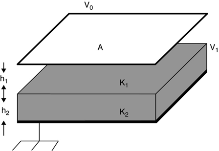
FIGURE 1.14 Two-dielectric-layer parallel plate capacitor.
For the ideal parallel plate capacitor, D is normal to the electrodes, and for a surface charge density σ on the bottom electrode, the total charge on the electrode is
from which
everywhere. The electric field is then

The voltages across the two layers are
and
from which
Since V 0 is the applied voltage to the top electrode, the capacitance is
From equation (1.46), the capacitance of the two layers as individual capacitors is

Substituting equations (1.72) into (1.71), we have derived the relationship for two capacitors in series:
1.8 Electric Dipoles
The dual-opposite-charge system shown in Figure 1.1b has something important missing. If two opposite-charge bodies are placed near each other, the Coulomb force will start pulling them together. What is missing is a mechanical support, or separator, of some sort that prevents the charges from moving. This separator can take many forms. It could be a dielectric slab through which the charges cannot move. It could exist at an atomic level — for instance, positive and negative charges may somehow be “pinned” in separate locations in a molecule of some sort. The molecule is electrically neutral, but it is made up of opposite charges somehow separated and held in place by the molecular structure itself.
However, when the charges are held apart, the electrical component of this structure is called an electric dipole or in context, simply a dipole.
Consider such a structure with the mechanical separating components having a (relative) dielectric constant of one. This lets us examine the electrical properties of dipoles without getting entangled in considerations of dielectric interfaces.
Figure 1.15 details an electric dipole with the supporting structure not shown. Charges +q and -q are located on the Y axis at Y = +L/2 and Y = -L/2, respectively.
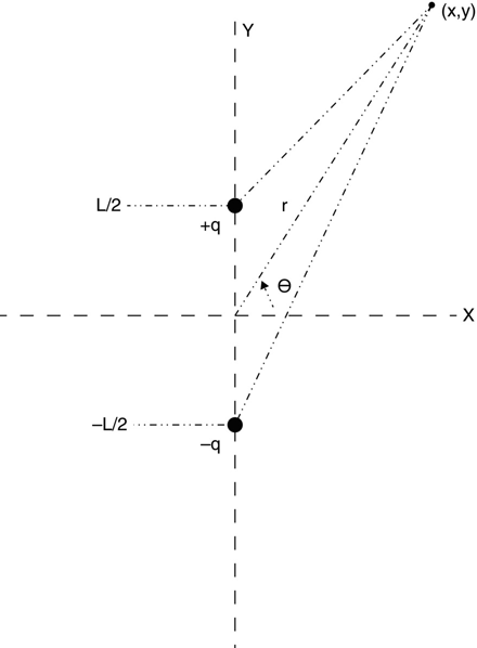
FIGURE 1.15 Structure of an electric dipole.
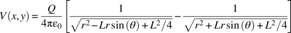
The voltage at any point (x,y) is simply
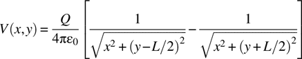
The same expression may, of course, be written in polar coordinates:
If r is much larger than L, equation (1.75) may be approximated by

or
The voltage is a function of r and θ, as expected. At θ = 0 or π (along the X axis), it is exactly zero, as symmetry demands. For any value of θ, the voltage falls off with the square of r. Far from an electric dipole [where distance (“far”) is measured in units of L], the dipole does not have much electrostatic influence as compared to separated charge (“separation” is also measured in units of L).
If an electric dipole is placed in a uniform electric field, there will be no net translation (movement of the center of gravity of the system) force on the dipole. The force trying to move the dipole in the direction of the field will be exactly canceled by the force trying to move the dipole against the direction of the field.
A dipole will rotate in a uniform electric field so as to align itself with the field. If we define the vector L as the line from charge -Q to charge +Q, then we can define the dipole moment as
and then the dipole torque in the uniform field is
As equation (1.79) predicts, the torque is maximum when the dipole is normal to the field (along the X axis in Figure 1.16) and zero when the dipole is aligned with the field (along the X axis in Figure 1.17).
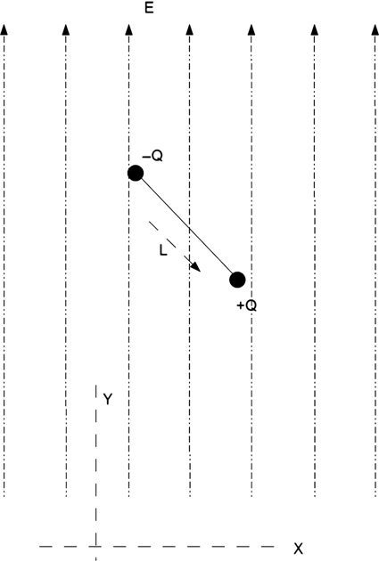
FIGURE 1.16 Electric dipole in a uniform field.
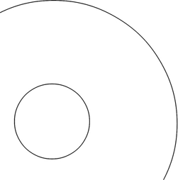
FIGURE 1.17 Section of concentric circles demonstrating a nonuniform field.
Figure 1.17 depicts a situation with a nonuniform electric field. Concentric circular (cross sections of long cylinders) electrodes were chosen for this example because the field lines can be drawn exactly without getting embroiled in calculations.
In this geometry all of the field lines are identical in that they are radial and all have the same magnitude–radius relationship. The nonuniform characteristic of these lines is that no two of them will point in the same direction; remember that two vectors have to agree in magnitude and direction for them to be identical. More complex geometries can be chosen in which the field lines differ in magnitude and direction, but this “extra” characteristic is not necessary for the point of this discussion.
In the situation depicted in the figure, two effects take place concurrently. First, as in the previous example, the dipole will rotate so that the -Q side is pointing toward the higher potential electrode—in this case the inner circle.
The electric field between two circles exhibits a monotonically decreasing magnitude (with increasing r). Once the dipole has rotated so that its -Q side is at a smaller radius than is its +Q side, the -Q side will feel a stronger force pulling it toward the inner circle than the +Q side will feel pulling it to the outer circle. The dipole, while aligning itself with the field lines, will move towards the center electrode (assuming, of course, that it is not being held in place in some way). This effect is called dielectrophoresis.6
Uncharged particles in a fluid will move in a uniform electric field, due to a complex interaction of the surface of the particle collecting a charge from the fluid while the fluid immediately surrounding the particle becomes charged opposite to the particle; the entire system, of course, remains neutral. This phenomenon is called electrophoresis.7
1.9 The Case for Approximate Numerical Analysis
All of the examples presented thus far have been for simple structures with helpful symmetries. The availability of such structures is good for exemplifying solving the equations that have been presented and examining some of these solutions. On the other hand, we must admit that these examples were not chosen only because they provide compact illustrative examples but because it is almost impossible to solve these equations formally for anything except very simple, highly symmetric, structures.
Classical texts are replete with solution techniques and problems that have been solved.8 These are important in that they extend our knowledge of the mathematics and the physics of electrostatics. On the other hand, most situations that commonly arise in practice are either totally unsolvable by any of these techniques or would require months of analysis to produce a solution.
As an example of this situation, consider Figure 1.18. We begin with a strip of metal on the top of a slab of dielectric that is fully metalized on its bottom face. For reasons that will be discussed in Chapter 2, we are interested in the capacitance between these two electrodes and the peak electric field (as a function of the applied voltage). This fairly straightforward situation is already a very difficult problem to attack analytically.
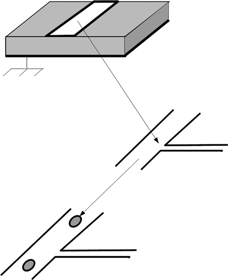
FIGURE 1.18 A common conductor–dielectric structure.
Now let’s add a narrow upper conductor strip branching off the original center conductor. What has happened to the capacitance and the peak electric field? Finally, we’ll add some holes in the upper conductor metalization. At this point we are beyond the capability of an analytic solution.
This example, although somewhat contrived, is actually indicative of real-world issues. Modern electronic devices, such as cellphones, make use of multilayer circuitboard technology. Many layers of dielectric and electrode patterns are sandwiched together into a thin circuitboard structure. Scattered about the board are holes passing from some layer to another. The walls of these holes are metalized; the metal on intermediate electrode layers is cleared away from the holes to prevent accidental contact. Again, the capacitances and peak electric fields are of significant interest: not only the nominal values but the variations in these values with manufacturing tolerances of metal patterns, dielectric thickness, metal patterning alignment errors, and so on.
In general, we need techniques for studying these issues. Changes in geometry must be input parameters that can be varied easily.
The numerical techniques to be presented in the following chapters are not the only techniques available for solving electrostatic problems. They are, however, indicative of two basic approaches: approximating either (1) the charge on electrodes for specified voltages on the electrodes or (2) the voltages in space for specified voltages on the electrodes. In both cases we replace a partial differential equation with a set of linear algebraic equations, which we know very well how to solve. The results are, of course, approximate, but by solving problems that have been solved (or approximated) analytically, we know that excellent accuracy can be obtained.
The approach chosen to present these materials will be somewhat different from that used in many texts. Rather than moving quickly to mathematical sophistication and generalization, we will stay as much as possible with the basic approaches and exploit these approaches to demonstrate the problems that they can solve. The goal here is not to present an exhaustive treatment of the approaches but rather to set up and solve many useful problems with the least sophisticated method possible in each case. If we succeed, this book should complement rather than duplicate the other books available in the literature.
Many concepts in electrostatics, such as image charges, are introduced in the chapters where these concepts fit logically with the analyses being performed. The decision to do this rather than introduce them in this chapter was based on the desire for brevity of this initial chapter—only those topics that are needed to proceed were covered.
Problems
1.1 Two small spheres of mass m are suspended from weightless strings of length L. The suspension points are a distance S apart. The spheres are charged as a capacitor; that is, Q is removed from one sphere and placed on the other. The spheres will move toward each other as shown in Figure P1.1.
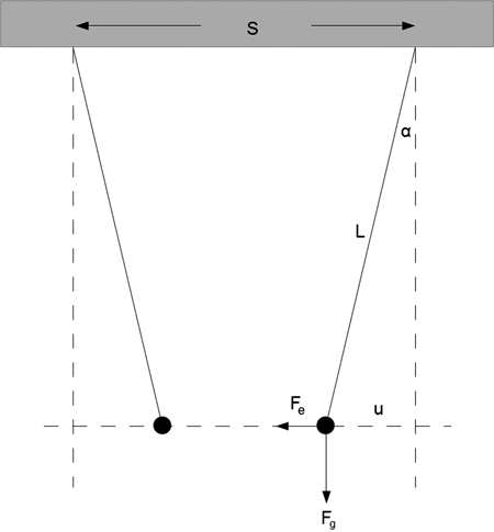
FIGURE P1.1 Two suspended charged spheres, Problem 1.1.
-
- By establishing for equilibrium the force of gravity and the Coulomb force, find the suspension angle α as a function of Q.
- What is the voltage between the spheres as a function of Q?
- What is the smallest angle α can assume (for nonzero Q)?
1.2 Repeat Problem 1.1a by finding the total potential energy of the structure and minimizing it.
1.3 Three small charged spheres are located as shown in Figure P1.3. One sphere is fixed at X = 0 with a charge of -1 (arbtirary units), one sphere is fixed at X = 10 with a charge of -3, and the third sphere is free to move on the X axis, with a charge q. What is the equilibrium position x for this system, and does it matter whether q is positive or negative?
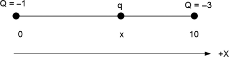
FIGURE P1.3 Layout for Problem 1.3.
1.4 Miniature chip capacitors are often constructed by building up successive layers of conductors and dielectric (typically a ceramic material) and then interconnecting the conductors, as shown in Figure P1.5. In these devices, the thickness : lateral dimensions ratio is low enough that we may use the ideal parallel plate capacitor calculation with good results. If the dielectric thickness between successive conductor layers is h, then the capacitance (per unit area) of the device is
where
- k = relative dielectric constant
- h = dielectric thickness between the metal layers
- n = number of dielectric layers
Suppose that we are allowed a total capacitor thickness of 3 mm. Each metal layers is 0.1 mm thick. We have a choice of dielectrics with relative dielectric constant ranging from 1 to 100. Unfortunately, however, the breakdown field of the dielectrics varies with k as
and the capacitor must be able to withstand 100 V. Find the maximum attainable capacitance per unit area, along with the values of n and k to achieve this maximum capacitance.
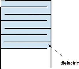
FIGURE P1.5 A multilayer chip capacitors.
1.5 Figure P1.6 shows a quadrupole charge configuration (Figure P1.6). Note that is also possible to define a linear quadrupole configuration. For r > > L, derive an approximation for the voltage as a function of r and ϕ.
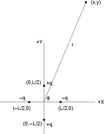
FIGURE P1.6 A quadrupole charge configuration.
1.6 An ideal parallel plate capacitor has a plate separation y. Calculate the force pulling the plates together under two conditions: (a) constant charge on the plates; (b) constant voltage on the plates.
References
- 1. J. D. Jackson, Classical Electrodynamics, 3rd ed., Wiley, New York, 1999.
- 2. G. F. Nicholson, An introduction to the rationalized M.K.S. system of units, Br. J. Appl. Phys. 2: 177 (1951).
- 3. S. Ramo, J . Whinnery, and T. Van Duzer, Fields and Waves in Communication Electronics, Wiley, New York, 1965.
- 4. J. McKelvey, Solid-State and Semiconductor Physics, Harper & Row, New York, 1966.
- 5.
http://en.wikipedia.org/wiki/Van_de_graaf_generator. - 6.
http://en.wikipedia.org/wiki/Dielectrophoresis. - 7.
http://en.wikipedia.org/wiki/Electrophoresis. - 8. W. Smythe, Static and Dynamic Electricity, McGraw-Hill, New York, 1950.