
4
Examples Using the Method of Moments
4.1 A First Modeling Program
We are now in a position to actually write a complete modeling program. We will use it to learn some more electrostatics, and then we will look at its limitations and inaccuracies and plan how we might improve it.
The basic components of this first program are as follows:
- Data input — we have to be able to “tell” the program what structure and what boundary conditions we want to examine.
- Data input processing — the program must be able to take the input data information and convert it into the subrectangles (cells) as described by the data input.
- Calculation of all the Li,j coefficients.
- Adding the extra row and column to the Li,j matrix (and the extra column to the V vector) as described in Chapter 3 to ensure that charge neutrality is maintained.
- Solving the linear equation set.
- Postprocessing and presentation of results — do we want capacitance, voltage, or electric field at some specific points?
- Warnings of possible inaccuracies from the program.
- Automatic improvements of the accuracy of the calculations.
Components 1 and 2 are in general a very sophisticated technology. We want our modeling software to be able to interact with our computer-aided design (CAD) software and extract necessary modeling information from the drawings as accurately and automatically as possible. This is a very important component of electrostatic (or general electromagnetic, mechanical, etc.) modeling. On the other hand, it is not a fundamental component of electrostatics or numerical electrostatic approximations. Our first modeling program will handle only very limited geometry descriptions, so we’ll begin with the brute-force path to data input—we’ll describe our geometry in a handwritten data file.
4.2 Input Data File Preparation for the First Modeling Program
We shall create a data file in which each line presents the minimum amount of information necessary to describe an electrode. The minimum amount criterion is intended to make life as simple as possible for the program user while letting the computer do the (necessary) repetitive work.
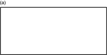
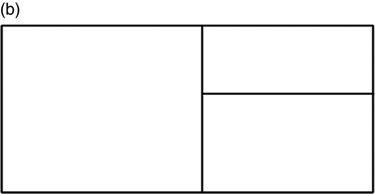

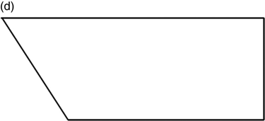
FIGURE 4.1 Basic rectangular modeling elements.
This program’s limitation is that our basic — and only — structure is a rectangle in the X–Y plane as shown in Figure 4.1a. It must be made up of square subsections. The side of each square, 2a, is the same for every rectangle in the dataset. The rectangle can be described as a single rectangle, or the same result can be obtained by describing several rectangles which combine to the same original rectangle, as in Figure 4.2b. This might seem like a waste of time and effort, but it is sometimes useful when a parameter study described by varying a dimension of one of the component rectangles is planned. Similarly, the electrode shown in Figure 4.1c is possible because it consists of rectangles.
On the other hand, the structure of Figure 4.1d is not allowed; it cannot be described by a combination of rectangles. (Note: This is not a fundamental limitation of the method — only an imposed limitation in this chapter.)
It would not be difficult to add the ability to include rectangles in the X–Z and Y–Z planes. The purpose of this first program, however, is to introduce all the aspects of building a modeling program and to learn some electrostatics from the results. Discussion of this capability will therefore be postponed to later chapters.
The default orientation of the input rectangles will be with their axes parallel to the X and Y axes. However, there is much to learn from structures with one or more electrodes rotated (in the X–Y plane), as shown in Figure 4.2.
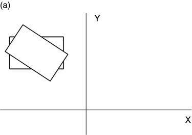
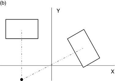
FIGURE 4.2 Rectangular electrode rotated in plane about an arbitrary point.
The most common rotation will be about the rectangle’s own center (Figure 4.2a), although the more general case of a rotation about an arbitrary point will be considered later in this chapter.
Rotation capability will be anticipated by including the required information in each data line, but our first program will ignore this information.
The first line (row) in the file shown in Table 4.1 contains the value of a. The program’s internal constants will use meters for the measure of length, so a should be specified in meters.
TABLE 4.1 Complete Data File for a Parallel Plate Capacitor
| 0.125 | ||||||
| 0.0 | 0.0 | 4 | 4 | 0 | 0.5 | 0 |
| 0.0 | 0.0 | 4 | 4 | 1 | -0.5 | 0 |
Each remaining line in the program (an arbitrary number of lines) contains the description of a rectangular electrode. This description assumes that the electrode’s sides are parallel to the axes, even though rotation will be considered later on.
For each line, the entries, in the order shown, are as follows:
- X0,Y0 = center of electrode
- Nx,Ny = number of cells in x and y that make up this rectangle
- h = height (z value) of rectangle in X–Y plane
- V = voltage applied to electrode
- θ = rotation information, not used yet
The total structure, as shown in Figure 4.3, is of two identical square plates, each subdivided into 16 square plates. The plates are one unit apart (the individual Z values don’t matter here; only the difference between them) with a voltage difference of one volt between them (the individual V values don’t matter here; only the difference between them.
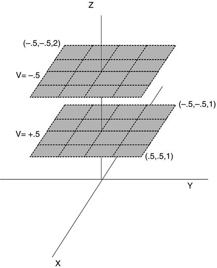
FIGURE 4.3 Capacitor layout described by Table 4.1.
The data file may be prepared by any ASCII text editor and saved to any convenient file name. A typical file extension for text files such as .txt is recommended but not required.
4.3 Processing the Input Data
The MATLAB function get_data.m reads the input file and produces two arrays, an array that contains the information needed to generate the Li,j array and an array containing the V data. This modeling program will use only the corrected single-point approximation (the empirical formula) for the off-diagonal Li,j terms. The information needed is therefore the location of the center of each rectangle and its size. In keeping with prior definitions, a subrectangle's dimensions are 2a × 2b; the a and b values are calculated and stored.
The following get_data.m program returns the arrays data_prep and volts:
function [a, data_prep, volts] = get_data()
% get_data gets the user created data file and converts it to
% a file of cells
% getdata2 assumes a uniorm nx and ny so that there is only 1 a and 1 b

filename = uigetfile('*.txt'), % read the file
xfid = fopen(filename);
all_data = (fscanf(fid, '%g'))';
nr_lines = (length(all_data) - 1)/7;
closeresult = fclose(fid)

a = all_data(1);
data_in = [];           % parse the data
for i = 1:nr_lines
 j = 7*(i-1) + 2;
 data_in = [data_in; all_data(j:j + 6)];
end

volts = [];
data_prep = [];
for i = 1:nr_lines        % loop through data file and build output
 x0 = data_in(i,1); y0 = data_in(i,2); nx = data_in(i,3); ny = data_in(i,4);
 x_ll = x0 - a*nx; x_ur = x0 + a*nx;
 y_ll = y0 - a*ny; y_ur = y0 + a*ny;

% x_ll = data_in(i,1);  x_ur = data_in(i,2);
% y_ll = data_in(i,3);  y_ur = data_in(i,4);
h = data_in(i,5); V = data_in(i,6); theta = data_in(i,7)*pi/180;
 for j = 1:nx
  xj = x_ll - a + j*2*a;
  for k = 1:ny
   yj = y_ll - a + k*2*a;
   if theta == 0
    line = [xj, yj, h];
   else
    % These 3 lines are for rotated electrode calculations
    x_new = xj*cos(theta) - yj*sin(theta);
    y_new = xj*sin(theta) + yj*cos(theta);
    line = [x_new, y_new, h];
   end
   data_prep = [data_prep; line];
   volts = [volts; V];
  end
 end
end
end
Table 4.2 shows these arrays for the dataset of Table 4.1.
| X0 | Y0 | h | V |
| -0.375 | -0.375 | 2 | 0.5 |
| -0.375 | -0.125 | 2 | 0.5 |
| -0.375 | 0.125 | 2 | 0.5 |
| -0.375 | 0.375 | 2 | 0.5 |
| -0.125 | -0.375 | 2 | 0.5 |
| -0.125 | -0.125 | 2 | 0.5 |
| -0.125 | 0.125 | 2 | 0.5 |
| -0.125 | 0.375 | 2 | 0.5 |
| 0.125 | -0.375 | 2 | 0.5 |
| 0.125 | -0.125 | 2 | -0.5 |
| 0.125 | 0.125 | 2 | 0.5 |
| 0.125 | 0.375 | 2 | 0.5 |
| 0.375 | -0.375 | 2 | 0.5 |
| 0.375 | -0.125 | 2 | 0.5 |
| 0.375 | 0.125 | 2 | 0.5 |
| 0.375 | 0.375 | 2 | 0.5 |
| -0.375 | -0.375 | 1 | -0.5 |
| -0.375 | -0.125 | 1 | -0.5 |
| -0.375 | 0.125 | 1 | -0.5 |
| -0.375 | 0.375 | 1 | -0.5 |
| -0.125 | -0.375 | 1 | -0.5 |
| -0.125 | -0.125 | 1 | -0.5 |
| -0.125 | 0.125 | 1 | -0.5 |
| -0.125 | 0.375 | 1 | -0.5 |
| 0.125 | -0.375 | 1 | -0.5 |
| 0.125 | -0.125 | 1 | -0.5 |
| 0.125 | 0.125 | 1 | -0.5 |
| 0.125 | 0.000 | 1 | -0.5 |
| 0.375 | -0.375 | 1 | -0.5 |
| 0.375 | -0.125 | 1 | -0.5 |
| 0.375 | 0.125 | 1 | -0.5 |
| 0.375 | 0.375 | 1 | -0.5 |
The order of the cells generated is arbitrary and inconsequential. The volts array and the data_prep array, however, must both have the cells in the same order. Each line in data_prep presents a cell; its center (xj,yj) and its height above z = 0 (zj). The volts array presents the applied voltage at each subrectangle. The two arrays could have easily been combined, but ultimately the matrix solution setup will require them to be separate arrays, so they were constructed separately from the start.
4.4 Generating the Li,j Array
The following is the L_fit.m program:
function L = L_fit(a, data_prep)
%function L = L_pt_corr(a, b, xi, yi, zi)
% This is the empirical function fit

% xj, yz, zj is the center of the source rectangle in the xyplane
% xi, yi, zi is the field point

global eps0

xi = data_prep(:,1);
yi = data_prep(:,2);
zi = data_prep(:,3);

n = length(xi);  % all the lengths are the same
xs = (repmat(xi,1,n) - repmat(xi',n,1)).^ 2;
ys = (repmat(yi,1,n) - repmat(yi',n,1)).^ 2;
zs = (repmat(zi,1,n) - repmat(zi',n,1)).^ 2;

p = 1.414*a;
La = (log((a + p)/a)/a - log((-a + p)/a)/a);

r = sqrt(xs + ys + zs);

L = r + 1/La./(1 + r/a);
L = 1./L/(4*pi*eps0);

end
The MATLAB function L_fit.m, with the data_prep array for its information, produces the Li,j coefficients using the empirical derived in Chapter 3. The function is vectorized so that no explicit loops are seen. Since the empirical formula returns La when r the field point is in the center of the source rectangle, the entire matrix of points can be calculated using this formula.
The main script for this program, mom1.m, assumes the task of adding the extra row and column to the Li,j array and the extra column to the volts array as specified in Chapter 3.
4.5 Solving the System and Examining Some Results
The mom_1.m program is as follows:
% This is the first MOM program with refining added

global eps0
eps0 = 8.854;
% Read the input file and process it into cell data
% Data Format:

[a, data_prep, volts] = get_data;

% Generate the L data
 L = L_fit(a, data_prep);

 nr_vars = length(L);
 new_col = L(1,1)*ones(nr_vars,1);
 L = [L, new_col];
 new_row = [new_col',0];
 L = [L; new_row];

 volts = [volts;0];
 q = Lvolts;

 cap = 0;
 for i = 1:length(q) - 1
  if q(i) > 0
   cap = cap + q(i);
  end
 end

 q
 cap
When mom_1.m solves the set of linear equations, the result is the vector q of the charges on each subelectrode. Remember that the last entry in q is actually a scaled voltage reference number—it is not the charge on any subelectrode. Ignoring this last entry, there are 32 entries, 16 for the first electrode and 16 for the second electrode.
Figure 4.4 shows the charge on the top electrode. The charge on the bottom electrode is a mirror image with the sign reversed.
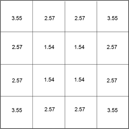
FIGURE 4.4 Charge distribution on a simple parallel plate capacitor.
Since the voltage difference between the two electrodes is 1 V, the capacitance is the sum of all the charges shown in Figure 4.4, C = 28.5 pF. The parallel plate capacitance for this structure is
Is a capacitance of >3 times the parallel plate capacitance reasonable? In other words, does this simulation make sense? Also, we see that the charge distribution is lowest in the center of the electrodes, higher at the edges, and highest at the corners. Is this physically possible and reasonable?
Before answering these questions, let’s get some more data. By reducing a but increasing nx and ny, we can increase the number of subelectrodes uniformly.
Figure 4.5 shows the result of this exercise. As n increases, the capacitance increases, leveling out at approximately 29.74 pF.
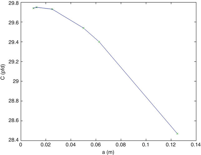
FIGURE 4.5 Capacitance C versus nx = ny for the simple two-electrode capacitor.
Figure 4.6 is a contour plot of the electrode charge for a fairly high resolution (n = 50) calculation.
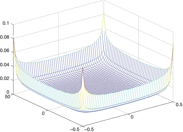
FIGURE 4.6 High-resolution plot of charge distribution on a parallel plate capacitor.
Figure 4.6 shows in much greater detail the story that Figure 4.4 was trying to tell. The highly mobile charge on an electrode pushes charge out to the edges because there is no counterbalancing (repulsive) charge at the edge to push back. This effect is much more significant in the corners because there is a lack of counterbalancing charge in two dimensions rather than in only one dimension, as there is away from the corners along an edge. The corner of an electrode in this capacitor forms a right angle.
4.6 Limits of Resolution
Figure 4.6 makes a clear case for higher-resolution calculations, the result is more accurate.
Making all of the cells as small as possible is not the only way to achieve good accuracy. There is no inherent reason why all the cells must be of the same size. We could start with all equal-size cells, examine our results, and then subdivide cells where the charge is the highest.
Figure 4.7 shows an example of the results of such a calculation. Using a threshold of some multiple of the minimum charge on the electrode, cells with a sufficiently high charge are simply subdivided into four smaller squares. The existing program must first be augmented so that each line in the data_prep array carries its own value of a, and then the chosen lines in data_prep each are replaced by four lines describing the new squares.
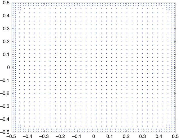
FIGURE 4.7 Refined dataset for simple capacitor example.
Figure 4.7 graphically shows what the new dataset would look like for this example. In this figure each dot represents the center of a (square) cell.
Figure 4.8 shows the program results for the a = 0.01 dataset as h is reduced from 1.
Figure 4.8 shows the ratio of the calculated capacitance to the ideal parallel plate capacitor capacitance. The figure shows that this ratio approaches 1 as the distance between the two electrode plates decreases. What is happening here in terms of the electric field deserves some discussion.
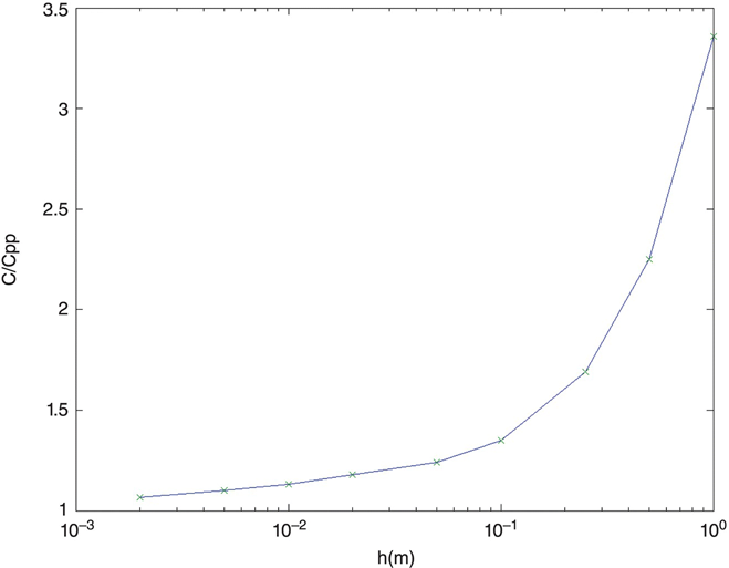
FIGURE 4.8 Example of ratio of capacitance to ideal parallel plate capacitance as height h decreases.
First, however, consider the situation when the plates are pulled farther and farther apart (see Figure 4.9).
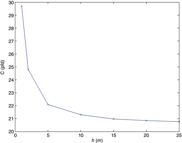
FIGURE 4.9 Example capacitance as h increases.
As is expected, C decreases as h increases. However, C does not fall toward zero but levels off at ~20.5 pF. At some point each electrode loses its effect on the charge on the other electrode. This is the self-capacitance discussed in the problem set for Chapter 3.
4.7 Voltages and Fields
Once the charge distribution in a structure is known, we can approximate the voltage anywhere in space by assuming that the charge in each cell is concentrated at the center of the cell. Then, the voltage Vi at point (xi,yi,zi) is given by
where
Figure 4.10 shows the equipotential surfaces at the center of the electrodes for the capacitor (Figure 4.3) with square electrodes of side 1, electrode separation = 1. These data were taken with a program run at nx = ny = 50. As the symmetry requires, the plane z = 0.5 is an equipotential at V = 0. This will prove important in subsequent discussions.
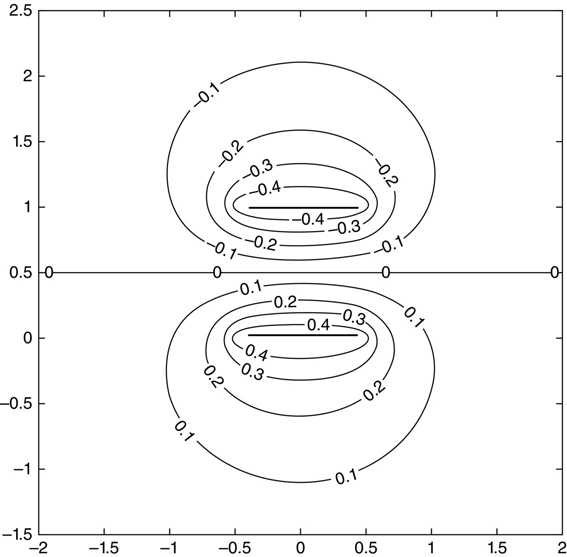
FIGURE 4.10 Equipotential surfaces for capacitor with h = 1.
Equation (4.2) is reasonably accurate provided the field point (i) is not too close to one of the charges. If this occurs, the voltage will approach infinity as point i approaches point j. This problem can be avoided by replacing the problematic term in equation (4.2) with a numerical integral (assume that the charge is distributed uniformly over its cell) or alleviated by using an empirical formula such as the one used in Chapter 3 for calculating Li,j.
The magnitude of the electric field at point i, with the same assumptions and caveats as described above, is
The X component of E is
and therefore

with corresponding expressions for Ey and Ez.
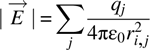
Figure 4.11 is a repeat of Figure 4.10 with electric field lines superimposed on the equipotential surfaces. Since this is the X–Z plane at the center (in y) of square electrodes, Ey = 0, so these field lines are showing the full picture.
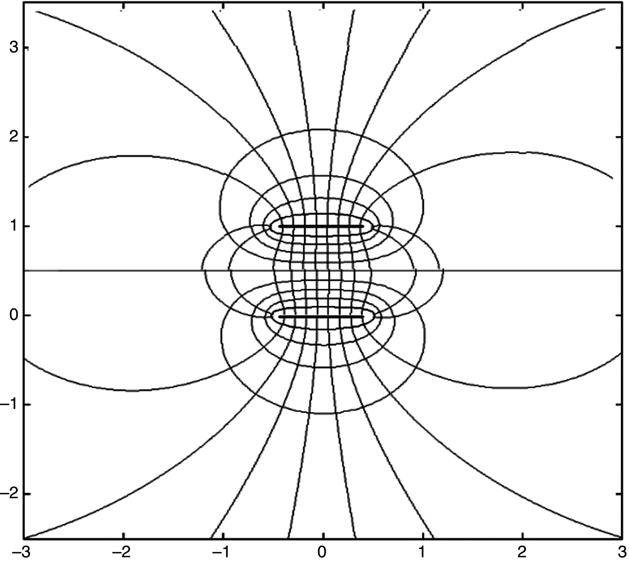
FIGURE 4.11 Electric field magnitude lines superimposed on equipotentials of Figure 4.10.
Note that there is significant field outside the region between the electrodes. This is why the capacitance is greater than the ideal parallel plate capacitance. The majority of the electric field energy not stored between the plates is due to field lines terminating at or near the edges of the electrodes, referred to as fringe, or fringing fields.
Figure 4.12 shows the equipotential surfaces for the same capacitor but with h (the plate separation height) decreased from 1.0 to 0.1. The electric field lines are not shown in this figure, but this omission is really inconsequential because the tightly bunched equipotentials between the electrodes and the widely spaced equipotentials elsewhere tell us that the electric field energy is concentrated principally between the electrodes and we should expect a capacitance close to the parallel plate capacitance.
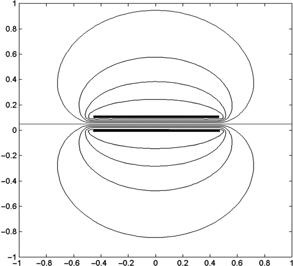
FIGURE 4.12 Equipotentials for a tightly spaced parallel plate capacitor.
Figure 4.5 showed that as the capacitor plates are separated, at h = 5 the capacitance has dropped to ≈ 22 pF and on further plate separation, the capacitance asymptotically approaches ≈ 20.5 pF. At h = 5 we would therefore expect the equipotential surfaces to show us electrodes that still see the effects on each other, but only slightly. Figure 4.13 illustrates this point exactly. For a single electrode we would expect approximately elliptically shaped curves near the electrode, with the curves becoming circular farther away from the electrode.
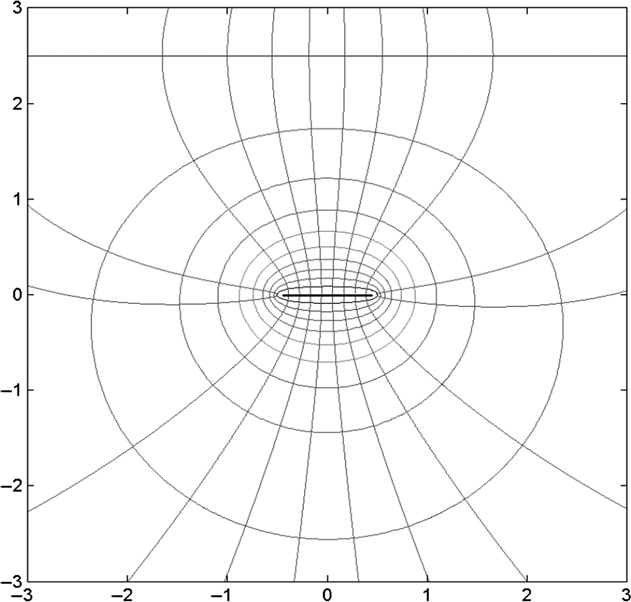
FIGURE 4.13 Equipotentials for widely spaced parallel plate capacitor.
4.8 Varying the Geometry
Various characteristics of the simple capacitor structure can be examined quite easily simply by changing numbers in the data file. For example, Figure 4.14 shows a cross section of the capacitor with one electrode offset (in X) with respect to the other. This offset is accomplished just by changing the first number in either the second or the third line of the file.

FIGURE 4.14 Cross section of capacitor with one electrode offset.
Figure 4.15 shows the results of the electrode offset for two values of h (the electrode separation). When h = 0.1, the capacitance falls almost linearly with xoffset, falling to approximately 25% of its original value, until xoffset = 1. At this point the two electrodes are no longer facing each other at all, and the capacitance decline with increasing xoffset levels off, falling to approximately 21 pF at xoffset = 3. This latter capacitance is, of course, the same capacitance that was approached in Figure 4.9, which showed the capacitance as the two electrodes were pulled apart (h increased). This make physical sense because electrodes that are too far apart to “see” each other don't know in which direction their greatest separation distance occurs.
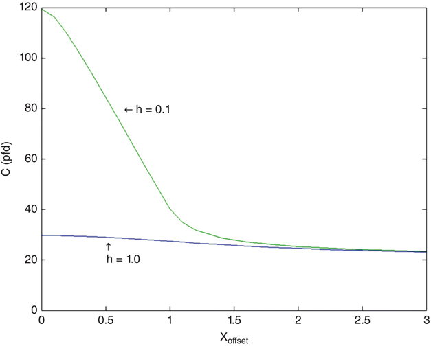
FIGURE 4.15 Parallel plate capacitance versus electrode offset.
When h = 1.0, the capacitance was already close to its maximum plate separation distance, so we see very little change as xoffset is increased. At xoffset = 3, we can't see the difference between the h = 1.0 and the h = 0.1 cases because, again, each electrode no longer knows where the other one is.

FIGURE 4.16 Capacitor with different-size square electrodes.
Figure 4.16 shows another possible variation. In this case both electrodes are kept square and centered, but the size of one of the electrodes is varied. Figure 4.17 shows the results of these variations when h = 0.1.
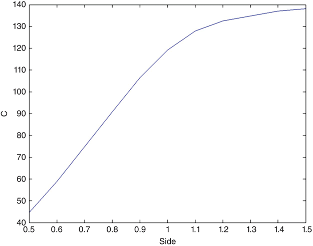
FIGURE 4.17 Capacitance of the capacitor shown in Figure 4.16.
There is no reason why either of the electrodes has to be square, or why different-size electrodes and misorientation cannot be combined.
Figure 4.18 shows a capacitor with connecting leads brought out. In this example the electrodes are rectangular and the two connecting leads do not have the same dimensions.
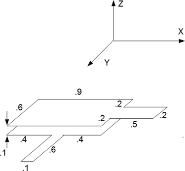
FIGURE 4.18 Capacitor with two different connecting leads.
Table 4.3 shows the data file for mom1.m that creates this capacitor.
TABLE 4.3 Data File for Capacitor Shown in Figure 4.18
| 0.01 | ||||||
| 0 | 0 | 45 | 30 | 0 | -0.5 | 0 |
| 0 | 0.6 | 5 | 30 | 0 | -0.5 | 0 |
| 0 | 0 | 45 | 30 | 0.1 | 0.5 | 0 |
| 0.7 | 0 | 50 | 10 | 0.1 | 0.5 | 0 |
The format of the file is the same as in the previous examples. All dimensions are in meters.
The first line in the data file is the cell ![]() side, a = b = 0.01. The second line describes the electrode of the lower section. The third line describes the connecting lead to this (lower) electrode. The geometry description (center and lengths) render it contiguous with the lower electrode, but this is not necessary for the program to operate correctly—the two pieces could be separate in space. The fourth and fifth lines describe the upper electrode and its connecting lead, respectively. The calculated capacitance is 76.7 pF. If we remove the connecting lines (lines 3 and 5 in the data file), the calculated capacitance drops to 69.2 pF. This is approximately a 10% drop—this may or may not be important, depending on the application.
side, a = b = 0.01. The second line describes the electrode of the lower section. The third line describes the connecting lead to this (lower) electrode. The geometry description (center and lengths) render it contiguous with the lower electrode, but this is not necessary for the program to operate correctly—the two pieces could be separate in space. The fourth and fifth lines describe the upper electrode and its connecting lead, respectively. The calculated capacitance is 76.7 pF. If we remove the connecting lines (lines 3 and 5 in the data file), the calculated capacitance drops to 69.2 pF. This is approximately a 10% drop—this may or may not be important, depending on the application.
The final variation to be presented in this section is the calculation for a rotated electrode. The calculation is not difficult or involved; it was omitted in the original program because it might have been a distraction.
The following equations rotate a point (xj,yj,zj) about the z axis by an angle θ:
This code is implemented in get_data.m. It is not executed until a nonzero rotation is encountered
Figure 4.19 shows an example of an electrode rotating about its center. The data file used is shown in Table 4.4. Figure 4.20 shows the result of this rotation.

FIGURE 4.19 Capacitor with an electrode rotated about its center.
TABLE 4.4 Data File for Capacitor Shown in Figure 4.19
| 0.01 | ||||||
| 0 | 0 | 25 | 200 | 0 | -0.5 | 45 |
| 0 | 0 | 25 | 200 | 0.1 | 0.5 | 0 |
To rotate an electrode about an arbitrary point (either inside our outside of the electrode), it is necessary only to define that point as the center of the coordinate system.
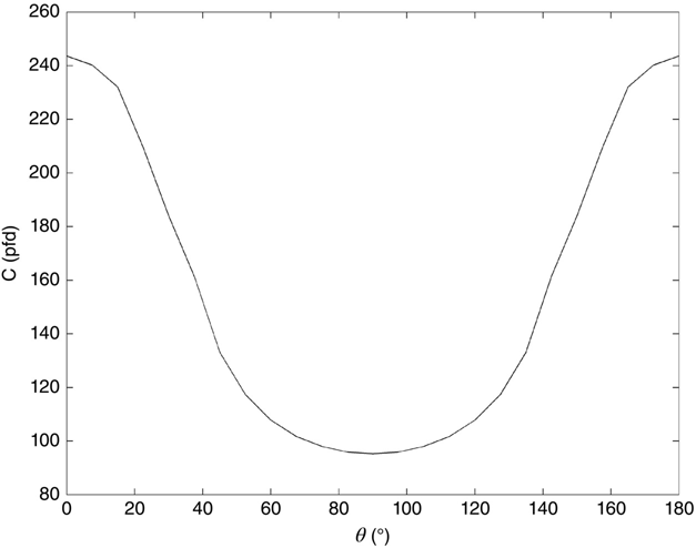
FIGURE 4.20 Capacitance as a function of rotation angle θ for capacitor shown in Figure 4.19.
Figure 4.21 shows an example of this situation; with respect to the origin, the lower left corner of the electrodes is (-0.25,–0.25). The data file is shown in Table 4.5, and the capacitance as a function of θ is shown in Figure 4.22.
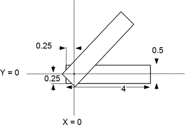
FIGURE 4.21 Capacitor with an electrode rotated about an arbitrary point.
TABLE 4.5 Data File for Capacitor Shown in Figure 4.22
| 0.01 | ||||||
| -0.25 | -0.25 | 20 | 160 | 0 | -0.5 | 45 |
| -0.25 | -0.25 | 20 | 160 | 0.1 | 0.5 | 0 |

FIGURE 4.22 Capacitance as a function of rotation angle θ for capacitor shown in Figure 4.21.
Figure 4.22 shows a curious capacitance behavior—while it is expected that the capacitance will fall drastically as θ is increased from 0, the capacitance variation near θ = 180 degrees might be unexpected. Examination of Figure 4.22, however, shows that this behavior is perfectly reasonable because of the electrodes’ overlay area as θ is varied.
The capacitor shown in Figures 4.21 and 4.22 is clearly a poor choice as a variable capacitor for tuning a radio or as a rotation angle encoder; monotonic capacitance versus rotation angle behavior is mandatory in these applications. This type of information is a very valuable result of simulation; we usually can forgive an absolute capacitance error of a few percent as long as this error repeats in a production environment, but surprises such as the behavior shown Figure 4.22, while educational in simulation, are often very costly once a design has been committed.
Problems
- 4.1 Create a dataset to analyze a square parallel plate capacitor with identical square electrodes 1 cm on a side and 1 cm apart. Use a resolution of a = 0.0002 m. Find the capacitance.
- 4.2 Modify the dataset of Problem 4.1 so that one of the electrodes has a square hole in the center, 0.2 cm on a side. Find the capacitance.
- 4.3 Show the charge density profile on both electrodes for the results of Problem 4.2.
- 4.4 Repeat Problems 4.2 and 4.3 with the same hole in both electrodes.
- 4.5 Calculate voltages and electric fields for (0,0,Z), that is, along the z axis for all of the cases described above.
- 4.6 Modify
mom1.mto locate the cells with the largest |q|, subdivide these cells so as to improve resolution, and recalculate the charge distribution and capacitance. Use the dataset from Problem 4.4 to demonstrate the results.