
Chapter 16
Electric Power Network Splitting Considering Frequency Dynamics and Transmission Overloading Constraints
Nelson Granda1 and Delia G. Colomé2
1Facultad de Ingeniería Eléctrica y Electrónica, Escuela Politécnica Nacional, Quito, Ecuador
2Instituto de Energía Eléctrica, Universidad Nacional de San Juan - CONICET, San Juan, Argentina
16.1 Introduction
Electrical Power System (EPS) security refers to the ability of the system to overcome imminent disturbances without loss of load. Security not only includes stability but also integrity and evaluation of EPS operation considering under/over voltages, under/over frequency, and overloads. Security control aims at decision making considering different time horizons and detail levels in order to prevent catastrophic contingencies and blackouts.
Controlled power system islanding is considered as the last emergency control action to halt failure propagation, avoiding uncontrolled power system separation and preventing wide area blackouts. In order to design a controlled islanding scheme (CIS), it is necessary to define electrical areas with adequate generation/demand balance and transmission facilities that can be opened. A global survey shows that controlled islanding schemes represent around 7% of protection schemes installed worldwide to safeguard EPS integrity [1]. A carefully planned and implemented controlled islanding scheme, besides preventing blackouts, allows: satisfying power demand for some users, maintaining operating generation facilities within safe limits, and assuring stable operation of the newly formed island through control actions that guarantee suitable variations of frequency, voltage, and current variables. In addition, power system restoration becomes more efficient when controlled islanding is applied first [2].
Several methodologies for controlled power system islanding proposed in the literature develop or use different algorithms and techniques to solve the problem; however, most of them can be synthesized in a two stage scheme: (i) Vulnerability Assessment and (ii) Islanding process, as shown in Figure 16.1.
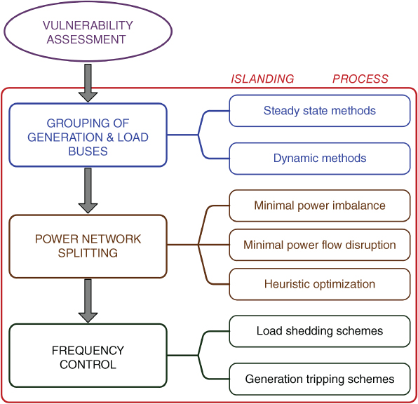
Figure 16.1 Synthesis of proposed methodologies for CIS.
16.1.1 Stage One: Vulnerability Assessment
The goal is to assess the risk level presented by an EPS during a specific static or dynamic operating condition regarding the occurrence of cascading events [3]. Additionally, vulnerability assessment determines the type and timing of control actions to be applied in order to avoid a system collapse. It must answer the following questions: When should the islanding process start? What are the variables to be monitored in order to define the onset of the islanding process? The analysis must consider possible contingencies and changes in operating conditions, establishing indicators to assess the vulnerability of the EPS [4].
16.1.2 Stage Two: Islanding Process
When vulnerability assessment points out that the power system is on the verge of collapse, the islanding process is started:
-
Grouping of generation and load buses: This involves determining the groups of generation and load buses that will shape the islands. Proposed approaches to grouping generation buses divide into: (i) Steady state methods, mainly based on power flow equations [5–7] and (ii) Dynamic analysis methods, which consider the dynamic characteristics of generators and loads as well as network topology [8–12].
Slow coherency has been the most used off-line approach to determine the Groups of Coherent Generators (GCG) in an EPS. However, system operation conditions change continuously during real-time: generation-load pattern, network topology, type, length, and place of faults can alter dynamic generator coherency. WAMS measurements enable dynamic behavior of EPS to be observed and might be used to assess generators' coherency during real-time operation. Due to the great amount of data delivered by WAMS, data mining and computational intelligence techniques are natural routes to solving the problem [13].
- Power network splitting: In this phase, transmission lines to be opened so as to form the islands are defined. Electric network partitioning is a complex optimization problem due to the unavoidable combinatorial explosion of the search space. Moreover, it is necessary to guarantee both speed and accuracy in determining the final islanding strategy. Proposed methods devised to solve the problem can be classified according to the objective function: (i) minimal power imbalance—this means minimizing the imbalance between generated and consumed active power into each island [5, 8, 10, 14–16]; (ii) minimal power flow disruption—the objective function minimizes the change of power flows at each island after system separation [17–20]; and (iii) heuristic optimization, which allows formulating complex objective functions with several variables to be minimized [21, 22]. Constrained spectral [19, 20] and multilevel recursive [15, 17] partitioning algorithms are the most promising candidates for the task.
- Frequency control: It is imperative to ensure integrity and survival of each island after system separation by controlling frequency, voltage, and current variables. The main proposed approaches focus on frequency control in each island after islanding through: (i) Under-frequency load shedding schemes (UFLS), and (ii) Generation tripping schemes (GTS). After islanding, it is virtually impossible to get islands with exact generation-load matching; for this reason UFLS is usually applied to balance active power and control excessive frequency excursions. In the case of islands with a generation surplus, only reference [8] proposes a methodology to control overfrequency by generation tripping; therefore, a GTS able to define the amount and place of generation to be tripped must be defined.
Assessment and control of overloaded transmission facilities after system islanding have not been adequately addressed in approaches proposed to date. Generally, it is assumed that there are sufficient resources to alleviate overloads; furthermore, changes in power injections aimed to control overloads may produce changes in active power balance and consequently in island frequency.
The present work introduces a new methodology to solve the power network splitting problem considering dynamic frequency behavior and overloading limits of transmission facilities. A network splitting mechanism based on the shortest path concept is devised to define the island boundaries; it takes into account active power imbalance constraints inside each island. Power imbalance constraint limits are determined based on maximum and minimum frequency deviations obtained by means of a reduced frequency response model. Load shedding and generation tripping schemes are defined in cases where the active power imbalance constraint is binding. Finally, an approach based on shift factors is used to determine the additional amount of load to be shed in order to alleviate possible overloads. The flowchart of the proposed methodology is shown in Figure 16.2.
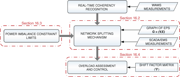
Figure 16.2 Flowchart of the proposed methodology.
In this chapter, it is assumed that vulnerability assessment and real-time generator coherency information is available and has been obtained by approaches [23, 24], respectively. This information is used as input to the proposed network splitting mechanism, introduced in Section 16.2.2. The methodology to determine limits for the active power imbalance constraint is presented in Section 16.3.2. After islands and tie-lines have been defined, the procedure applied to assess and alleviate overloaded transmission links is presented in Section 16.4. A study case is shown in Section 16.4.1, where the proposed methodology is applied to avoid system collapse due to cascade tripping. Finally, the main conclusions and recommendations for future work are given in Section 16.4.5.
16.2 Network Splitting Mechanism
The proposed network splitting mechanism belongs to the minimal power imbalance approaches and determines the composition of each island and the transmission lines that should be opened in order to feature the islands. Firstly, a simple weighted undirected graph of the EPS is obtained off-line and it is continuously reduced and refreshed in real-time with measured active power injections and network topology. Later, through a graph partitioning procedure, generation and load buses are assigned to each GCG—information delivered by the real-time coherency recognition stage—in such a way that the active power imbalance constraint is enforced. During this process, the amount of load or generation that must be shed in order to enforce the active power imbalance constraint into each island is calculated. Finally, tie-lines are determined through a search procedure.
Dynamic frequency behavior is indirectly considered through the power imbalance constraint. Allowed limits for frequency variation, imposed by the user or country technical codes, are translated into active power imbalance by means of analytical expressions obtained from the reduced frequency response model of each island [25]. The flowchart of the proposed network splitting mechanism is shown in Figure 16.3.
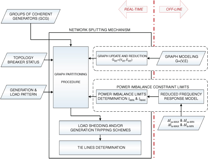
Figure 16.3 Flowchart of the network splitting mechanism.
Most of the calculations associated with the proposed approach are done in a real-time environment and fed with measurements data gathered by WAMS/PMU and SCADA/EMS: voltage and current phasors, frequency, generated and consumed active power, power flow in transmission facilities, and breaker status. Off-line computations are related to the procurement and identification of models to be employed in real-time, mainly a graph representation of the power network and a reduced model of the power-frequency control system of each generator.
16.2.1 Graph Modeling, Update, and Reduction
The procedure starts in an off-line environment, modeling the EPS through a simple weighted undirected graph G, as (16.1):
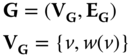
where VG is the vertices set with its weights w(v) that represents power system buses and net active power injection on each bus, respectively; EG is the edges set with its weights w(e) that represents power system transmission links and their distance measures as defined in (16.2), respectively. In transmission networks, line resistance is usually small and can be neglected.
Later, in a real-time environment, the graph G is continuously refreshed with generation-load patterns and breaker status data. The updated graph GRT is conveniently reduced following the guidelines in [26]:
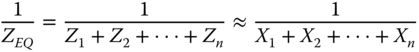
- Equivalence of parallel lines: This is applied when two or more transmission links are connected between two buses u and v; the equivalent impedance is calculated by (16.3):
16.3
- Removal of degree-one nodes: This is the case of radial connected buses, where the interconnection link between buses u, and v is removed as well as bus v. In order to maintain the active power balance after graph reduction, it is necessary to move the active power injection PINJ from the radial bus v to the upstream bus u adding the active power losses PLOSS in the removed transmission link.
- Removal of degree-two nodes: This is the case of switching substations, where net active power injection is zero. The equivalent impedance is calculated by (16.4):
16.4
- Removal of step-up transformers: This is a particular case of degree-one node removal, where the active power injection is the generated active power. The aforementioned reduction rules are illustrated in Figure 16.4.
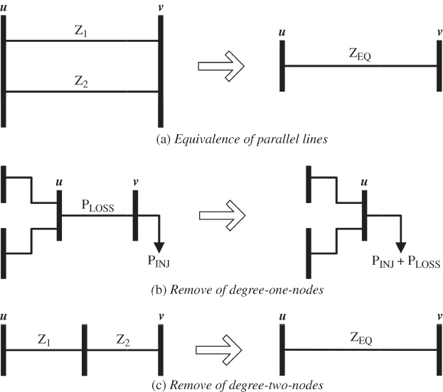
Figure 16.4 Graph reduction rules.
16.2.2 Graph Partitioning Procedure
In this stage, the updated and reduced graph GRT will be divided into a number of islands equal to the number of GCGs. First, generators of each GCG are sorted in descending order according to their pre-disturbance generated active power PG, and all buses are labeled as unvisited. Through a recursive allocation procedure, load buses are appended to the closest GCG. Starting with the first GCG, the generator with the largest generated active power PG is chosen as the pivot generator and labeled as visited. Then the closest load bus to the pivot generator is calculated considering the impedance magnitude as edge weight. Finding the closest load bus implies a minimization problem, given by (16.5), and Dijkstra's shortest path algorithm is used because of its calculation speed [27]:
where Djk denotes a vector with the shortest paths between pivot generation bus BGj and load buses BLk, and NL is the number of non-visited load buses. When the impedance magnitude (16.2) is used as edge weight, the graph partitioning procedure assigns only the closest electrical buses into each island. The closest load bus to the pivot generator is added to the GCG and labeled as visited.
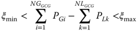
Each time a new load bus is added to a GCG, it is imperative to make sure that the active power imbalance constraint (16.6) is not binding. This means that the active power imbalance on each island—total generated active power minus total assigned load demand—remains within limits ξmax, ξmin. Cases where the active power imbalance constraint is binding are solved by means of UFLS and GTS, as explained in Section 16.3.1.1.
Limit values (ξmax, ξmin) determine the frequency behavior on each island: wider limits imply greater frequency variations on each island, and less load to shed when tripping tie-lines to create the islands.
The recursive allocation procedure concludes when all generators have been checked as visited, whereupon a connectivity check is performed in order to find isolated load buses, which will be added to the closest GCG as explained in the next paragraph. The flowchart of the graph partitioning procedure is presented in Figure 16.5.
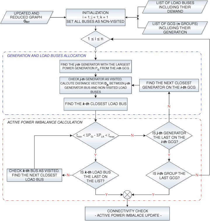
Figure 16.5 Graph partitioning procedure.
16.2.3 Load Shedding/Generation Tripping Schemes
When a disturbance produces the tripping of generation or load facilities, the active power balance is broken, so that some loads cannot be served by the online generators and are not visited during the recursive allocation procedure. These loads are attached to the closest GCG according to (16.7), where Dkj denotes a vector with the shortest paths between pivot load bus BLk and generation buses BGj, and NG is the number of generation buses.
The active power excess provided by these buses must be shed. In the case of a generation surplus, those generators that should be tripped can also be identified. The amount of active power generation or load to be tripped is defined by the active power imbalance constraint limits and has no relation with traditional UFLS or GTS.
16.2.4 Tie-Lines Determination
After all load buses have been attached to a specific GCG, it is possible to determine the tie-lines that need to be opened in order to create the islands. A search procedure is used to look for transmission lines whose endpoints belong to a different GCG, to become tie-lines.
16.3 Power Imbalance Constraint Limits
Maximum (ξmax)and minimum(ξmin) values for the active power imbalance constraint on each island are determined by means of analytical expressions derived from the reduced frequency response model, which essentially represents the average response of all generators in the island following a generation/load imbalance [28]. Inter-machine oscillations during a disturbance are ignored by the model; however, results are still valid since only coherent generators are put together into each island.
Several approaches have been proposed to calculate frequency behavior after a disturbance that produces active power imbalances in the EPS; the most popular are:
- Analytical expressions and nomograms [29–31], which are easy to use and fast to calculate, but the results are approximate.
- Time-domain simulation of the complete EPS model [32–34], including full speed regulator-prime mover models, boiler dynamics, turbine conduit dynamics, AGC, and so on. These approaches provide the exact frequency response with computational costs that can be high depending on the size and complexity of EPS under analysis.
- Equivalent models of the power-frequency control system [25, 28, 35]—usually known as frequency response models—whose accuracy is similar to the simulation of the complete EPS model but with reasonable computational costs. Depending on the generator's technology, complex transfer functions might be used to model the turbine-governor set of each generator [36], obtaining the so called “complete frequency response model.” In this work, the frequency response model of every generator is reduced by using only a first-order approximation of the speed regulator-prime mover set, which allows using a “reduced frequency response model” of each island and formulating analytical expressions to calculate the maximum transient frequency deviation.
16.3.1 Reduced Frequency Response Model
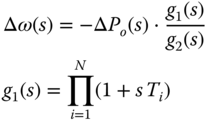
The dynamic frequency response of an isolated EPS following a generation-load imbalance ΔPO(s) can be calculated through a reduced frequency response model with: equivalent system inertia HEQ, generator's permanent droop Rj, and system load damping D. All dynamic models of speed regulators and prime movers are represented with an equivalent first-order model. The dynamic frequency response of the reduced model in the Laplace domain is given by (16.8):
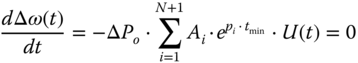
where Kmj, Fi, and Ti are parameters of the equivalent first-order model of speed regulator-prime mover of each generator [25]. These parameters are obtained by fitting the response of the equivalent first-order model to the response of the detailed dynamic model using a non-linear least-squares search method [37]. The time response of the reduced frequency response model is given by (16.9):
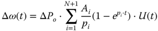
where Ai and pi denote poles and zeros of the transfer function (16.8), respectively. The time instant tmin when the maximum transient frequency deviation occurs is determined by taking the derivative of (16.9) and solving the resulting equation (16.10):
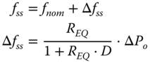
The maximum transient frequency deviation ΔfMAX is calculated by replacing tmin into (16.9). This model has been extended in order to include not only thermal but also hydraulic generators. The steady state frequency deviation Δfss after primary frequency regulation is calculated using (16.11), where REQ is the equivalent system droop of each island and is determined considering only those generators participating in primary frequency control.
The application domain of each model is shown in Figure 16.6, where thin continuous lines correspond to frequency on each bus given by the time-domain simulation of the full EPS model. It can be seen that before 4 s, the time evolution of the complete frequency response model and the reduced model are identical; however after this moment they drift apart. The aforementioned models' response fits well with the frequency evolution obtained by time-domain simulation. The maximum transient frequency deviation obtained by solving (16.8), (16.9), and (16.10) is represented with a diamond. Finally, the steady state frequency deviation obtained with (16.11) agrees well with the steady state frequency obtained by time-domain simulation.
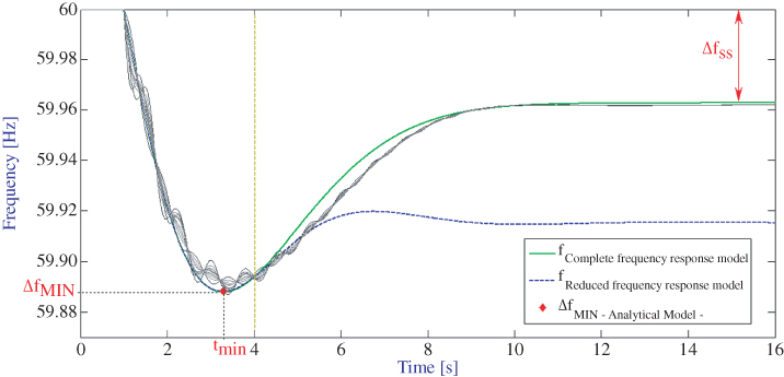
Figure 16.6 Frequency response model application domain.
16.3.2 Power Imbalance Constraint Limits Determination
Using (16.9)–(16.11) for the maximum transient and steady state frequency deviation, the power imbalance constraint limits (ξmax, ξmin) are calculated. As input to the procedure, values of the maximum allowed steady state frequency deviation (Δfss-MAX) and maximum allowed transient frequency deviation (Δfts-MAX) are needed. Usually, these values are defined by country regulations, for example, ENTSO-E standards dictate that, for Continental Europe, the maximum steady state frequency deviation shall be ±200 mHz and the maximum instantaneous frequency deviation shall be ±800 mHz [38]. The procedure to determine active power constraint limits ξmax and ξmin is shown in Figure 16.7.
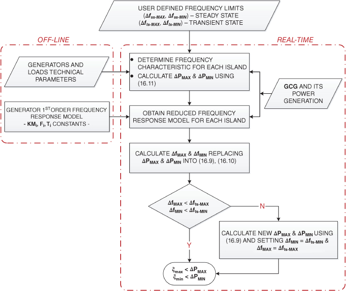
Figure 16.7 Power imbalance constraint limits determination.
First, the active power imbalance (ΔPMAX) that produced the maximum allowed steady state frequency deviation (Δfss-MAX) is calculated using (16.11). The obtained ΔPMAX value is then introduced in (16.9) and (16.10) in order to determine the maximum expected transient frequency deviation (ΔfMAX) on each island. If ΔfMAX is less than Δfts-MAX, this implies that a smaller active power imbalance will produce transient and steady state frequency deviations less than those defined by the user, and consequently ΔPMAX becomes the upper limit ξmax for the active power imbalance constraint. On the other hand, if ΔfMAX is greater than Δfts-MAX then (16.9) is used to calculate a new ΔPMAX value, thereby ensuring that frequency deviations remain under user defined limits. In this case, new ΔPMAX value becomes the upper limit ξmax for the active power imbalance constraint.
The whole procedure is repeated for determining the lower limit ξmin for the active power imbalance constraint, where minimum allowed steady state frequency deviation (Δfss-MIN) and minimum allowed transient frequency deviation values (Δfts-MIN) are used.
16.4 Overload Assessment and Control
So far, generation, load, and topology of each island have been determined. A DC power flow is used to assess overloads on each island and a procedure based on shift factors is employed to determine the amount of load to be shed in order to alleviate the expected overloads. EPS facilities have different overloading levels depending on their constructive characteristics. The proposed scheme aims to control transmission link overloads that must be relieved in short time periods, which is the case for devices based on power electronics such as FACTS, HVDC stations, and power converters associated with solar and wind generation.
The procedure described below is applied to each island and starts with calculation of shift factor matrix Ψ through (16.12), where B is the diagonal branch susceptance matrix, B− is the reduced nodal susceptance matrix, and A− is the reduced incidence matrix. In reduced matrices A− and B−, the column corresponding to the system slack bus is filled with zeros.
The shift factor matrix Ψ, also known as the transmission sensitivity matrix, gives the variations in flow for each line due to changes in the nodal injections, with the slack bus assumed to ensure the real power balance. The shift factor matrix is a function of the transmission element susceptances and network topology [39]. A calculation alternative is to estimate matrix Ψ from PMU measurements in real-time, as proposed in [40].
After this, active power flows Pu-v are calculated by (16.13), where Pinj is the vector of active power injections on each bus. In the case of overloaded transmission links, the surplus power flow ΔPu-v is determined using (16.14), where Pu-v and Pu-vMAX are the calculated and maximum power flow of the transmission link, respectively.
A set of Nb load buses participating in load shedding must be defined according to their entry values in Ψ; those buses with higher shift factors are candidate buses for load shedding. Remember that element ![]() of matrix Ψ represents the sensitivity of the flow on line u-v to a change in the power injection at bus i; therefore, shedding load in bus i with the highest element
of matrix Ψ represents the sensitivity of the flow on line u-v to a change in the power injection at bus i; therefore, shedding load in bus i with the highest element ![]() will produce the biggest change in flow of line u-v.
will produce the biggest change in flow of line u-v.
The surplus power flow ΔPu-v is distributed among the candidate buses Nb through factor FDi calculated by (16.15), that weights individual bus demand with respect to total demand that will be shed. Finally, the real amount of load (PLiLshd) to be shed on bus i is obtained by (16.16):
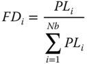
Reactive power to be shed (QLiLshd) on bus i is determined considering that the power factor remains constant, so that (16.17) holds:
The use of DC power flow involves knowing in advance the shift factor matrix Ψ. Calculating Ψ implies computing matrices B, B−, and A− as shown in (16.12); the computational cost of Ψ can be important when considering a large EPS. One way to speed up the calculation of Ψ associated with each island is to determine periodically (on line) the matrix Ψ of the entire EPS before separation into islands. Then, in real-time, the matrix Ψ associated with each island is calculated through elementary matrix operations on the entire system matrix Ψ, as proposed in [41], accelerating the DC power flow calculation process. Overload assessment and control based on DC power flow delivers good results; however, when high reactive power flows in the network, results may be conservative.
16.5 Test Results
The IEEE 10-machine 39-bus test system (New England system) is used to simulate a cascade tripping of transmission lines with the subsequent loss of stability and system collapse. Through the application of the proposed methodology, the system collapse is averted, keeping the main electrical variables within normal operating limits. Generator 10 is modeled as a hydraulic unit in order to show the performance of the reduced frequency response model to predict transient frequency deviations. A traditional UFLS scheme, whose first step trips at 59.4 Hz, is also modeled. The test system is shown in Figure 16.8.
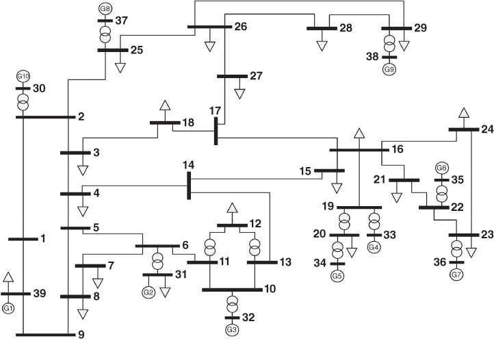
Figure 16.8 Test system—IEEE New England 10-machine 39-bus system.
16.5.1 Power System Collapse
The power system is feeding a total load of P = 5478.3 MW, Q = 1178.6 Mvar, and under these circumstances the trip of line 14-15 at 0.2 s, due to a three-phase fault, causes the overload and subsequent tripping of line 03-04 at 10 s. The cascade tripping produces two electrical areas tied by a radial link. Vulnerability assessment, implemented as proposed in [23], determines that the areas lose synchronism at 12.18 s with subsequent system collapse. The difference between the Center of Inertia (COI) angle of each area and the COI angle of the entire system is used as stability index: when the index value exceeds 180 degrees, it is said that the area is unstable.
Time evolution of generator rotor angles is shown in Figure 16.9 with thin continuous lines, while the thick continuous line represents system COI angle evolution (δCOI). Dotted and dashed lines depict the COI-referred rotor angles of areas 1 (δArea1-COI) and 2 (δArea2-COI), respectively. It can be seen that the COI-referred rotor-angle corresponding to area 2 reaches 180 degrees difference first. It can be observed that after tripping of line 03-04 at 10 s, the system separates into two electrical areas. The time evolution of frequency in all buses is depicted in Figure 16.10, where a similar separation into two areas is also observed.
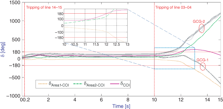
Figure 16.9 Collapse case—COI-referred and generator rotor angles [deg].
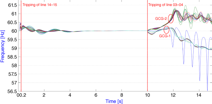
Figure 16.10 Collapse case—Bus frequency [Hz].
16.5.2 Application of Proposed Methodology
After the trip of line 03-04, the real-time coherency recognition procedure identifies GCG-01 = {G1,G2,G3} and GCG-02 = {G4,G5,G6,G7,G8, G9}. This grouping is consistent with the network topology, since after tripping of line 03-04, generators {G1,G2,G3} are connected with the remaining system through a weak radial interconnection (line 01-02 and line 01-39).
Input values for the tolerance limits determination procedure are: Δfss-MAX = 60.4 Hz, Δfss-MIN = 59.6 Hz, Δfts-MAX = 61.0 Hz and Δfts-MIN = 59.4 Hz. It is noteworthy that maximum and minimum transient frequency limits corresponds to over-speed protection of generators and UFLS settings, respectively. Applying the procedure described in Section 16.3.2 to Island 1, it is found that the power imbalance ΔPMIN obtained when considering Δfss-MIN = 59.6 Hz produces an expected transient frequency deviation greater than the minimum allowed (ΔfMIN > Δfts-MIN). This means that after EPS splitting, frequency in Island 1 will drop beyond 59.4 Hz, triggering the first step of the traditional UFLS. Therefore, a new value for ΔPMIN is calculated by setting ΔfMIN = Δfts-MIN = 59.4 Hz, and the result becomes the lower limit for the power imbalance constraint in Island 1. In Island 2, maximum and minimum expected transient frequency deviations are within the specified limits.
The frequency evolution on each island is presented in Figure 16.11; time-domain simulation results of the complete frequency response model are represented with solid lines, and maximum and minimum transient frequency values obtained by solving (16.8)–(16.10) are represented by diamonds. The agreement between the two models is remarkable: frequency error is less than 0.1% and time error is less than 1.5 %. The proposed procedure to determine power imbalance constraint limits allows the coordination between traditional UFLS and CIS. User can define minimum transient frequency deviation after islanding in such a way that traditional UFLS does not act or triggers only up to a certain step.
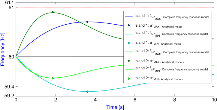
Figure 16.11 Frequency deviation—Complete and analytical frequency response models [Hz].
After finishing the recursive allocation procedure (Figure 16.5), power imbalance into each island lies between calculated limits; however, the connectivity check determines that load bus 4 is isolated and cannot be added to Island 2 because there is no possible electrical connection between them. Therefore, load bus 4 is added to Island 1 with a consequent change in the power imbalance. The load shedding/generation trip procedure determines that 785.2 MW of load must be tripped in Island 1 so that frequency stays within the user specified limits. Island 2 is generation rich and 490 MW of generated power in bus 37 must be tripped to avoid triggering over-speed protections. Finally, the tie-line determination procedure establishes that line 01-02 will be tripped. The aforementioned loads, generator, and tie-line are tripped together at 11.5 s, before the system loses synchronism.
Once the islands have been determined, the overload assessment procedure shows that line 05-06 is overloaded. Following the procedure stated in Section 15.4, an additional 83 MW of load are shed in buses 4 and 8 in order to alleviate the overload. A side effect of this additional load shedding is that minimum transient and final steady state frequencies increase.
Results obtained with the proposed methodology are summarized in Table 16.1. In the first part, maximum and minimum values for transient as well as steady state frequency deviation are shown. In the second part, the active power imbalance evolution through each stage of the network splitting mechanism is shown. Stages of active power imbalance updating are: Graph Partitioning Procedure (GPP), Connectivity Check (CC), and Load Shedding/Generation Trip Schemes (LS/GT) for frequency and overload control. Finally, in the third part, control actions are detailed, including additional load shedding at buses 4 and 8 for overload control.
Table 16.1 Results of the proposed methodology
| ISLAND 1 | ISLAND 2 | ||||
| ANALYTICAL FREQUENCY RESPONSE MODEL | |||||
| ΔPMAX = | 430.2 | [MW] | ΔPMAX = | 736.6 | [MW] |
| Δfss-MAX = | 0.40 | [Hz] | Δfss-MAX = | 0.40 | [Hz] |
| Δfts-MAX = | 0.71 | [Hz] | Δfts-MAX = | 0.90 | [Hz] |
| a ΔPMIN = | −228.1 | [MW] | ΔPMIN = | −355.1 | [MW] |
| Δfss-MIN = | −0.21 | [Hz] | Δfss-MIN = | −0.40 | [Hz] |
| Δfts-MIN = | −0.38 | [Hz] | Δfts-MIN = | −0.44 | [Hz] |
| ACTIVE POWER IMBALANCE EVOLUTION | |||||
| GPP | −127.2 | [MW] | GPP | 277.2 | [MW] |
| CC | −1013.3 | [MW] | CC | 1163.3 | [MW] |
| LS/GT | −228.1 | [MW] | LS/GT | 673.3 | [MW] |
| CONTROL MEASURES | |||||
| Load Shedding Scheme | Generation Tripping Scheme | ||||
| Bus | Load | Generator | Generated Power | ||
| 4 | 301.4 + 48 | [MW] | 37 | 490 | [MW] |
| 7 | 32 | [MW] | |||
| 8 | 164.3 + 35 | [MW] | |||
| 12 | 3.5 | [MW] | |||
| 31 | 4.6 | [MW] | |||
| 39 | 279.5 | [MW] | |||
| Total | 868.3 | [MW] | Total | 490 | [MW] |
a Minimum transient frequency is set to 59,4 Hz, according to specified limits and ΔPMIN is calculated thereafter.
The dynamic performance of the main system variables after controlled system islanding is included in Table 16.2. These values were obtained by time-domain simulation of the full power system model. Maximum and minimum transient frequency deviation after islanding are shown in the first part of the table, while the steady state magnitudes (at 40 s of simulation) of frequency and voltages are presented in the second part.
Table 16.2 Dynamic performance of main system variables
| ISLAND 1 | ISLAND 2 | ||||
| fMIN [Hz] | 59.53 | [Hz] | fMIN [Hz] | 60.1 | [Hz] |
| fMAX [Hz] | 60.21 | [Hz] | fMAX [Hz] | 60.79 | [Hz] |
| f 40s [Hz] | 59.72 | [Hz] | f 40s [Hz] | 60.26 | [Hz] |
| VMIN, 40s [pu] | 0.991 | [pu] | VMIN, 40s [pu] | 1.000 | [pu] |
| VMAX, 40s [pu] | 1.055 | [pu] | VMAX, 40s [pu] | 1.048 | [pu] |
The frequency in Island 1 after system separation is above 59.4 Hz, thus avoiding activation of the traditional UFLS scheme. This is an important advantage considering that an unexpected disturbance could lead the recently formed island to the collapse; a traditional under-frequency load shedding scheme would act as backup protection system. Steady state frequencies and voltages are within normal operation limits except on bus 1 (VMAX, 40s = 1.048 pu), which becomes a radial bus without load (Ferranti effect). Similarly, maximum and steady state frequency values in Island 2 are within normal operating limits, and the same observation applies to voltages. Time evolution of voltage magnitude and frequency on each bus, and lines loadability obtained by time-domain simulation, are shown in Figure 16.12, Figures 16.13 and 16.14, respectively.
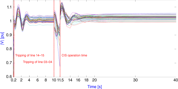
Figure 16.12 Proposed ACIS—Bus voltage magnitude [pu].
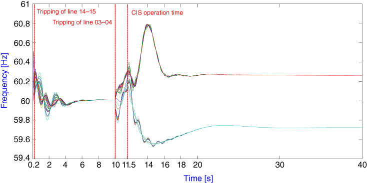
Figure 16.13 Proposed ACIS—Bus frequency [Hz].
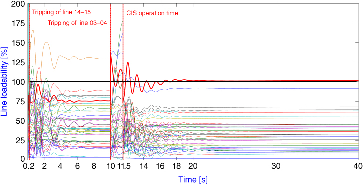
Figure 16.14 Proposed ACIS—Line loadability [%].
16.5.3 Performance of Proposed ACIS
All simulations were performed using MATLAB® 2014a software running on Windows 7® (64-bit) platform, processor Intel i7® [email protected] Ghz with 4 GB RAM memory. Total computation time is 0.12 s (7.2 cycles on 60 Hz). Power imbalance constraint limits and network splitting procedures are the most demanding, taking approximately 98% of total computation time. Overload assessment and control is fast and easy to implement, using only 2.4% of total computation time. A summary of computation times per phase of the methodology are shown in Table 16.3.
Table 16.3 Computation times summary
| Phase | Computation time | ||
| [s] | [%] | [60Hz - cycles] | |
| Power imbalance constraint limits determination | 0.0417 | 34.4 | 2.5 |
| Island 1 | 0.0205 | 16.8 | 1.2 |
| Island 2 | 0.0190 | 15.8 | 1.1 |
| Network splitting mechanism | 0.0756 | 63.2 | 4.5 |
| Overload assessment and control | 0.0028 | 2.4 | 0.2 |
| Total time | 0.1205 | 100 | 7.2 |
Reference [42] presents time delays associated with switching, protection, and control equipment installed in a real EPS to perform wide area control actions. Taking those values into consideration, total time needed to implement control actions dictated by the proposed CIS can be calculated as in (16.18):
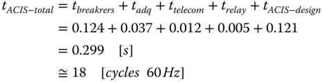
Reference [3] studies tripping times of out of step relays when applied to an IEEE New England 10-machine 39-bus system, and through time-domain simulations and Monte Carlo methods, it determines that: minimum tripping time is 0.8342 s, mean tripping time is 1.2252 s with standard deviation of 0 3746 s. Total time needed to implement proposed CIS is less than minimum tripping time of out of step relays, and therefore the proposed approach is capable of avoiding system collapse by acting before uncontrolled system separation.
16.6 Conclusions and Recommendations
Through the development and integration of novel algorithms and procedures for graph partitioning and frequency behavior estimation, a new approach for power system islanding has been presented. The proposed scheme is able to avoid a system collapse by splitting the system into electrical islands with adequate generation-load balance. The proposed methodology is a contribution to CIS development, improving its ability to determine the necessary control actions to divide the power system and to ensure islands' survival.
The scheme changes its settings automatically according to received real-time data, thus adapting its behavior to system operational conditions. The proposed CIS incorporates a dynamic constraint into the network splitting procedure and allows controlling the frequency on each island based on user specified limits. To the author's knowledge, this is the first controlled islanding scheme that incorporates a dynamic mechanism to define the tolerance of the power imbalance constraint.
Results using the proposed approach show that the frequency on each island can be effectively controlled within user defined limits. This feature allows coordinating actions between traditional UFLS and proposed CIS. An important issue when designing real-time algorithms is to reduce calculation times as much as possible. It was shown that power imbalance constraint limits and network partitioning procedures consume most of the calculation time. Due to its characteristics, the graph partitioning procedure could be implemented using parallel computing, where each generator is assigned to one core. The main implementation issues are related to hardware deployment through the power network in order to open the circuit breakers of generators, loads, and transmission lines. The proposed load shedding/generation trip schemes consider load as a continuous variable, but in a real EPS it is a discrete variable.
Current developments in Wide Area Monitoring, Protection and Control (WAMPAC) systems, and high performance computing open a way for future implementation of the proposed CIS. Further work includes an enhanced procedure for overload assessment and control using PMU measurements to estimate shift factors, and taking into account the reactive components of power flows. These advancements would improve the performance and adaptability of the procedure.
References
- 1 V. Madani, D. Novosel, S. Horowitz, M. Adamiak, J. Amantegui, D. Karlsson, et al., “IEEE PSRC Report on Global Industry Experiences With System Integrity Protection Schemes (SIPS),” Power Delivery, IEEE Transactions on, vol. 25, pp. 2143–2155, October 2010.
- 2 J. Q. Tortos and V. Terzija, “Controlled islanding strategy considering power system restoration constraints,” in Power and Energy Society General Meeting, 2012 IEEE, 2012, pp. 1–8.
- 3 J. C. Cepeda, “Evaluación de la Vulnerabilidad del Sistema Eléctrico de Potencia en Tiempo Real usando Tecnología de Medición Sincrofasorial,” PhD, Instituto de Energía Eléctrica - IEE, UNSJ, San Juan, Argentina, 2014.
- 4 H. Song and M. Kezunovic, “A new analysis method for early detection and prevention of cascading events,” Electric Power Systems Research, vol. 77, pp. 1132–1142, 2007.
- 5 C. G. Wang, B. H. Zhang, J. Shu, P. Li, and Z. Q. Bo, “A fast method for power system splitting boundary searching,” in Power & Energy Society General Meeting, 2009. PES '09. IEEE, 2009, pp. 1–8.
- 6 M. A. Anuar, U. Dorji, and T. Hiyama, “Principal Areas for Islanding Operation Based on Distribution Factor Matrix,” in Intelligent System Applications to Power Systems, 2009. ISAP '09. 15th International Conference on, 2009, pp. 1–6.
- 7 L. Yuanqi and L. Yutian, “Islanding cutset searching approach based on dispatching area,” in Power Engineering Conference, 2007. IPEC 2007. International, 2007, pp. 950–954.
- 8 J. Ming, T. S. Sidhu, and S. Kai, “A New System Splitting Scheme Based on the Unified Stability Control Framework,” Power Systems, IEEE Transactions on, vol. 22, pp. 433–441, 2007.
- 9 X. Wang, W. Shao, and V. Vittal, “Adaptive corrective control strategies for preventing power system blackouts,” in 15th Power Systems Computation Conference, Liège, Belgium, 2005.
- 10 H. You, V. Vittal, and W. Xiaoming, “Slow coherency-based islanding,” Power Systems, IEEE Transactions on, vol. 19, pp. 483–491, 2004.
- 11 X. Guangyue, V. Vittal, A. Meklin, and J. E. Thalman, “Controlled Islanding Demonstrations on the WECC System,” Power Systems, IEEE Transactions on, vol. 26, pp. 334–343, 2011.
- 12 S. M. Tabandeh and M. R. Aghamohammadi, “A new algorithm for detecting real-time matching for controlled islanding based on correlation characteristics of generator rotor angles,” in Universities Power Engineering Conference (UPEC), 2012 47th International, 2012, pp. 1–6.
- 13 C. Juarez, A. R. Messina, R. Castellanos, and G. Espinosa-Perez, “Characterization of Multimachine System Behavior Using a Hierarchical Trajectory Cluster Analysis,” Power Systems, IEEE Transactions on, vol. 26, pp. 972–981, 2011.
- 14 S. Kai, Z. Da-Zhong, and L. Qiang, “Splitting strategies for islanding operation of large-scale power systems using OBDD-based methods,” Power Systems, IEEE Transactions on, vol. 18, pp. 912–923, 2003.
- 15 C. G. Wang, B. H. Zhang, Z. G. Hao, J. Shu, P. Li, and Z. Q. Bo, “A Novel Real-Time Searching Method for Power System Splitting Boundary,” Power Systems, IEEE Transactions on, vol. 25, pp. 1902–1909, 2010.
- 16 P. A. Trodden, W. A. Bukhsh, A. Grothey, and K. I. M. McKinnon, “Optimization-Based Islanding of Power Networks Using Piecewise Linear AC Power Flow,” Power Systems, IEEE Transactions on, vol. 29, pp. 1212–1220, 2014.
- 17 L. Juan, L. Chen-Ching, and K. P. Schneider, “Controlled Partitioning of a Power Network Considering Real and Reactive Power Balance,” Smart Grid, IEEE Transactions on, vol. 1, pp. 261–269, 2010.
- 18 W. Xiaoming and V. Vittal, “System islanding using minimal cutsets with minimum net flow,” in Power Systems Conference and Exposition, 2004. IEEE PES, vol. 1, pp. 379–384, 2004.
- 19 L. Ding, P. Wall, and V. Terzija, “Constrained spectral clustering based controlled islanding,” International Journal of Electrical Power & Energy Systems, vol. 63, pp. 687–694, 2014.
- 20 J. Quiros-Tortos, R. Sanchez-Garcia, J. Brodzki, J. Bialek, and V. Terzija. (2014, Constrained spectral clustering-based methodology for intentional controlled islanding of large-scale power systems. IET Generation, Transmission & Distribution. Available: http://digital-library.theiet.org/content/journals/10.1049/iet-gtd.2014.0228
- 21 C. S. Chang, L. R. Lu, and F. S. Wen, “Power system network partitioning using tabu search,” Electric Power Systems Research, vol. 49, pp. 55–61, 1999.
- 22 L. Liu, W. Liu, D. A. Cartes, and I.-Y. Chung, “Slow coherency and Angle Modulated Particle Swarm Optimization based islanding of large-scale power systems,” Advanced Engineering Informatics, vol. 23, pp. 45–56, 2009.
- 23 J. C. Cepeda, J. L. Rueda, D. G. Colome, and D. E. Echeverria, “Real-time transient stability assessment based on centre-of-inertia estimation from phasor measurement unit records,” Generation, Transmission & Distribution, IET, vol. 8, pp. 1363–1376, 2014.
- 24 N. Granda, Colome D., “Real-Time identification of coherent generators using PMU measurements,” Energia Technical Magazine, vol. 8, pp. 76–84, 2012.
- 25 A. Denis Lee Hau, “A general-order system frequency response model incorporating load shedding: analytic modeling and applications,” Power Systems, IEEE Transactions on, vol. 21, pp. 709–717, 2006.
- 26 X. Guangyue and V. Vittal, “Slow Coherency Based Cutset Determination Algorithm for Large Power Systems,” Power Systems, IEEE Transactions on, vol. 25, pp. 877–884, 2010.
- 27 F. B. Zhan and N. C. E. , “Shortest Path Algorithms: An Evaluation Using Real Road Networks,” Transportation Science, vol. 32, pp. 65–73, Feb. 1998.
- 28 P. M. Anderson and M. Mirheydar, “A low-order system frequency response model,” Power Systems, IEEE Transactions on, vol. 5, pp. 720–729, 1990.
- 29 L. L. Fountain and J. L. Blackburn, “Application and Test of Frequency Relays for Load Shedding,” Power Apparatus and Systems, Part III. Transactions of the American Institute of Electrical Engineers, vol. 73, pp. 1660–1668, 1954.
- 30 C. F. Dalziel and E. W. Steinback, “Underfrequency Protection of Power Systems for System Relief Load Shedding-System Splitting,” Power Apparatus and Systems, Part III. Transactions of the American Institute of Electrical Engineers, vol. 78, pp. 1227–1237, 1959.
- 31 H. E. Lokay and V. Burtnyk, “Application of Underfrequency Relays for Automatic Load Shedding,” Power Apparatus and Systems, IEEE Transactions on, vol. PAS-87, pp. 776–783, 1968.
- 32 C. Evrard and A. Bihain, “Powerful tools for various types of dynamic studies of power systems,” in Proceedings of 1998 International Conference on Power System Technology, POWERCON 1998, pp. 1–6 vol. 1.
- 33 DIgSILENT GmbH, “DIgSILENT PowerFactory User Manual,” ed. Gomaringen, Germany,: DIgSILENT GmbH, 2013.
- 34 Siemens Power Transmission & Distribution Inc, “PSS/E 30.2 Users Manual,” ed. Schenectady, US: Siemens Power Transmission & Distribution Inc, 2005.
- 35 I. Egido, F. Fernandez-Bernal, P. Centeno, and L. Rouco, “Maximum Frequency Deviation Calculation in Small Isolated Power Systems,” Power Systems, IEEE Transactions on, vol. 24, pp. 1731–1738, 2009.
- 36 IEEE-PES Task Force on Turbine-Governor Modeling, “Dynamic Models for Turbine-Governors in Power System Studies,” IEEE, USA, PES-TR1, 2013.
- 37 L. Ljung. (2015). System Identification Toolbox: User's Guide (Online version ed.). Available: http://www.mathworks.com/help/pdf_doc/ident/ident.pdf
- 38 ENTSO-E, “ENTSO-E Network Code on Load-Frequency Control and Reserves (LFCR),” 28 June 2013. [Online]: https://www.entsoe.eu/major-projects/network-code-development/load-frequency-control-reserves/Pages/default.aspx. Accessed on 31-08-2017.
- 39 P. A. Ruiz, A. Rudkevich, M. C. Caramanis, E. Goldis, E. Ntakou, and C. R. Philbrick, “Reduced MIP formulation for transmission topology control,” in Communication, Control, and Computing (Allerton), 2012 50th Annual Allerton Conference on, 2012, pp. 1073–1079.
- 40 Y. C. Chen, A. D. Dominguez-Garcia, and P. W. Sauer, “Measurement-Based Estimation of Linear Sensitivity Distribution Factors and Applications,” Power Systems, IEEE Transactions on, vol. 29, pp. 1372–1382, 2014.
- 41 Y. Fu and Z. Li, “A Direct Calculation of Shift Factors Under Network Islanding,” Power Systems, IEEE Transactions on, vol. 30, pp. 1150–1551, 2014.
- 42 M. V. Flores, D. E. Echeverria, R. P. Barba, and G. Arguello, “Architecture of a systemic protection system for the interconnected national system of Ecuador ” in 2015 IEEE Asia-Pacific Conference on Computer Aided System Engineering (APCASE) Quito, Ecuador, 2015.