Chapter 18
Implementation of a Real Phasor Based Vulnerability Assessment and Control Scheme: The Ecuadorian WAMPAC System
Pablo X. Verdugo1, Jaime C. Cepeda2, Aharon B. De La Torre1 and Diego E. Echeverría1
1Research and Development Engineer, Technical Development Department, Operador Nacional de Electricidad, CENACE, Quito, Ecuador
2Head of Research and Development, Technical Development Department, Operador Nacional de Electricidad, CENACE, Quito, Ecuador
18.1 Introduction
With each passing year, the operation of electric power systems experiences several technical challenges associated with the new paradigms of management and planning such as the inclusion of deregulated markets, the interconnection with neighboring regional systems, the diversification of energy sources, the inclusion of environmental restrictions, and even the massive penetration of nonconventional generation plants. Under these conditions, security and reliability can be seriously compromised since unexpected disturbances may cause violations to the security limits established for the electric power system leading to the outage of important system elements and even partial or total blackouts [1].
Real time supervision of the static and dynamic security of the power system plays a fundamental role inside the applications used in control centers. The main purpose of real time monitoring is to present an early warning to the system operators so they can execute adequate control actions and thus mitigate potentially harmful stress conditions in the system. In this context, besides SCADA/EMS functionalities, it is necessary to include complementary technological solutions to evaluate and improve the security of the power system in real time; synchrophasor measurement systems (PMU/WAMS) are part of these technologies [2]. In addition, other Smart Grid applications have also been designed in order to perform self-healing and adaptive reconfiguration actions based on system-wide analysis with the objective of reducing the risk of power system blackouts.
Phasor Measurement Units (PMUs) are devices that allow the estimation of current and voltage synchrophasors in different areas of an electric power system. Their high precision, response speed, and time synchronization make PMUs viable equipment for monitoring the steady and dynamic states of an electric system and also for applications of protection and control within a Wide Area Monitoring, Control, and Protection (WAMPAC) system. The Ecuadorian National Interconnected System (SNI from the acronym in Spanish) is rather small, and up until 2003 it had no permanent connections with neighboring power systems. Nowadays, the Ecuadorian SNI maintains a synchronous connection with the Colombian system, which is a little less than three times larger in terms of load demand. Several issues have been presented in this interconnected system's operation, such as: oscillatory instability, large congestions in transmission power lines, and partial collapses due to single contingencies, to name but a few. It is in this connection that the need to implement a reliable monitoring system arose. Therefore, since 2010, the Ecuadorian ISO, CENACE, has undertaken a project to implement a WAMPAC infrastructure in Ecuador that facilitates the real time monitoring, supervision, and control of the Ecuadorian system through the use of synchrophasor measurements. This initiative was based on the current availability of synchronized phasor measurement technology for monitoring, in real time, highly stressed operating conditions that might eventually cause problems of steady-state angle or voltage stability, as well as oscillatory stability risks. Within the past few years, CENACE has concluded the first stage of the project, which consists in the installation of 30 PMUs around the SNI along with a complex optical fiber communication infrastructure and a sophisticated phasor data concentrator (PDC), administrated by the WAProtectorTM software developed by the Slovenian Company ELPROS. WAProtectorTM manages the PMU data via the intranet communication network, and it connects to the PMUs using the IEEE C37.118 communication protocol [3]. This platform constitutes CENACE's Wide Area Monitoring System (WAMS). Likewise, a smart infrastructure based on synchrophasor technology for real time control of N-2 critical contingencies has been also implemented in Ecuador. This redundant control scheme is made up of 58 relays with built-in PMU functionality. Together, these two technological infrastructures constitute the current Ecuadorian WAMPAC System.
18.2 PMU Location in the Ecuadorian SNI
One of the criteria used for determining the location of PMUs is system observability, whilst aiming to maximize redundancy by using the fewest PMUs without compromising the desired observability of the system. Several authors have developed mathematical models to determine optimal PMU placement in an electric system using optimization methods [4]. Another criterion for PMU placement relies on placing PMUs at the most important or most significant substation buses, although this is considered subjective since it depends on the information that is required for a specific analysis. As a starting point, PMU placement in the SNI was defined based on monitoring requirements, taking into consideration the most relevant buses in the Ecuadorian power system and the operating criteria. Once the initial WAMS was implemented and the first results were gathered, it was possible to either identify new areas for PMU placement or relocate the ones previously installed with the aim of obtaining full system observability not only related to steady-state conditions but also to dynamic system behavior. Therefore, the necessity of monitoring different areas that are considered to have a relatively high operative relevance, in order to perform a precise and reliable evaluation of the system performance, has been defined in a procedure for deciding further PMU locations. In general terms, the main objectives for installing PMUs in the SNI, which have been defined in CENACE's procedure, are:
- Supervising the real time dynamic operation of the SNI to allow the operators to take preventive actions when facing instability risks (early warning).
- Having more precise information and tools to perform stability analysis and determine the presence of poorly damped oscillation modes.
- Performing post-mortem analyses in order to evaluate the system behavior and then improve the procedures to restore the energy supply after fault events.
- Tuning of Power System Stabilizers (PSS) and validation of control systems models.
- Monitoring the most congested transmission corridors via steady-state angle stability and voltage stability assessment tools.
Once each PMU is located, the measured data is delivered to the control center where WAProtector enables PMU management and further power system analysis. Inside the WAProtector server, data analysis and real time assessment of system security, including the evaluation of steady-state and oscillatory stability phenomena, are carried out. The main applications available in WAProtector are: steady-state angle stability (phase angle difference), steady-state voltage stability of transmission corridors, oscillatory stability, islanding detection, harmonic distortion analysis, historic data, and system event analysis, among others. WAProtector's applications enable early-warning alerts when pre-specified thresholds are exceeded; however, these limits must be configured by the user. Therefore, it is necessary to specify an adequate reference framework to allow the monitoring of specific power system thresholds as regards each one of the available supervisory applications. In this connection, three methodologies were proposed by CENACE for determining adequate thresholds regarding: (i) phase angle difference, (ii) voltage profile power transfer of transmission corridors, and (iii) oscillatory issues. These limits are the referential framework for assessing stability in real time, and constitute indicators that give the operators real time early-warning signals of the possible risk of system stress conditions.
18.3 Steady-State Angle Stability
Angle stability refers to the ability of the synchronous machines of an interconnected power system to remain in synchronism after the system has been subjected to a disturbance. To maintain synchronization, it is necessary to keep or restore the balance between the mechanical and electromagnetic torques of each synchronous machine [5].
The angular difference between two buses of a power system is a direct measure of the transfer capacity between these nodes. Figure 18.1 illustrates two areas (A and B) of a power system interconnected through a set of electric branches.
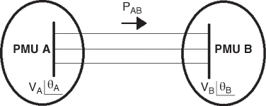
Figure 18.1 Power transfer between two system buses.
Assuming the “π” equivalent model for the set of branches between the two areas, presented in Figure 18.2, the power transfer between A and B is given by (18.1):
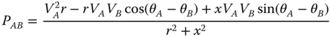
where VA and VB are the voltage phasor magnitudes at buses A and B, respectively; θA and θB represent voltage phasor angles at buses A and B, respectively; x is the series reactance between buses A and B; and r corresponds to the series resistance.
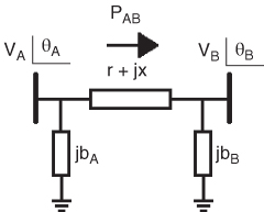
Figure 18.2 “π” equivalent of system branches.
Considering that ![]() in a high-voltage power system, (18.1) can be reduced to (18.2), whose graphic representation is depicted in Figure 18.3.
in a high-voltage power system, (18.1) can be reduced to (18.2), whose graphic representation is depicted in Figure 18.3.
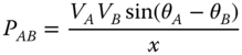
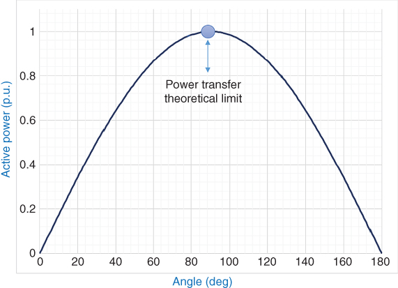
Figure 18.3 Power–angle curve.
Mathematically, maximum power transfer occurs when ![]() , that is when
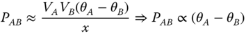
, that is when ![]() . Nevertheless, due to the complexity of the power system that can cause congestion in the transmission network, it is usually not possible to reach this theoretical limit. Thus, the maximum difference between nodal phase angles depends on the actual system topology, and it has to be computed for each electric power system. Considering that θA – θB usually presents small values in electric power systems that satisfy the steady-state angle stability constraint, the power flow transferred by the branch between buses A and B, as shown in (18.3), is proportional to the angle difference between these two buses:
. Nevertheless, due to the complexity of the power system that can cause congestion in the transmission network, it is usually not possible to reach this theoretical limit. Thus, the maximum difference between nodal phase angles depends on the actual system topology, and it has to be computed for each electric power system. Considering that θA – θB usually presents small values in electric power systems that satisfy the steady-state angle stability constraint, the power flow transferred by the branch between buses A and B, as shown in (18.3), is proportional to the angle difference between these two buses:
In this connection, the actual power transfer limit between buses A and B depends on the maximum phase angle difference between these nodes, and vice versa. Therefore, to determine the phase angle difference maximum limit (defined as steady-state angle stability limit), it is necessary to reach the power transfer limits through the transmission corridor. Thus, the monitoring of phase angle differences between the system buses gives the operator an early warning of potential system congestion. WAProtector has an application that allows monitoring the angle difference of phasor voltages at buses supervised by PMUs through advanced visualization applications. Figure 18.4 shows an example of the graphic display via dynamic contour plots of the angle difference in the SNI in real time. It is possible to observe how the contour of the Ecuadorian map turns into a light-gray like tone in correspondence with an increase of the congestion of the network and thus the growth of the angular difference. Additionally, the software allows setting the limit values of angle separation between buses, with the aim of providing the operator an adequate warning. These values correspond to the limits of steady-state angle stability, which should be properly determined.
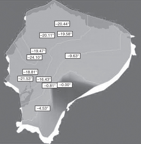
Figure 18.4 Dynamic Contour plot of angle differences.
As a starting point, it is necessary to define a reference bus (in this case, the Molino 230 kV substation, where one of the largest generation plants in Ecuador, Paute, is located), in order to give the operator an adequate reference as to provide an early warning of the risk of congestion, under the premise of maintaining the steady-state system security. The proposal consists of performing static simulations to assess the most critical power transfer conditions in the SNI, considering the potential occurrence of N-1 contingencies and the gradual increase of nodal loads on particular system areas. The proposed mechanism of analysis is to simulate, by means of power system simulator software (DIgSILENT PowerFactory in this case), the behavior of the power transfers under different operating conditions (high and low hydrological scenarios with low, medium, and high demand conditions), including contingency analysis and the gradual increase of load. The approach presented in Figure 18.5 is proposed to this end. The methodology begins with the definition of scenarios. Subsequently, case studies that include the operational conditions to be analyzed are prepared. Then, a DPL (DIgSILENT Programming Language) script is executed that controls an iterative N-1 contingency analysis of several transmission elements associated with gradual increases of load in specific areas (50 previously defined critical contingencies are simulated). This analysis allows reaching high-stress system conditions, and thus determining the maximum angular separation between the 230 kV buses of the Ecuadorian SNI and the Molino substation. Interested readers can find further explanation of this methodology in [2].
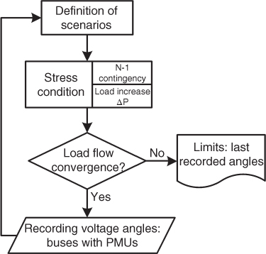
Figure 18.5 Methodology for determining the steady-state angle stability limits.
The mean (μ) of the established maximum angular differences is the alert limit. Moreover, the alarm limit corresponds to the sum of the mean and one standard deviation (σ) of the sample. This is based on the criterion that at least 50% of the analyzed values should be included within the range of the standard deviation around the mean (![]() ), known as Chebyshev's inequality [6]. As an illustration, Figure 18.6 presents the resulting histogram of the angle differences between Pascuales and Molino 230 kV buses for high hydrological scenarios. Additionally, Table 18.1 summarizes the results of alert and alarm limits for all SNI buses with PMUs for high hydrological scenarios.
), known as Chebyshev's inequality [6]. As an illustration, Figure 18.6 presents the resulting histogram of the angle differences between Pascuales and Molino 230 kV buses for high hydrological scenarios. Additionally, Table 18.1 summarizes the results of alert and alarm limits for all SNI buses with PMUs for high hydrological scenarios.
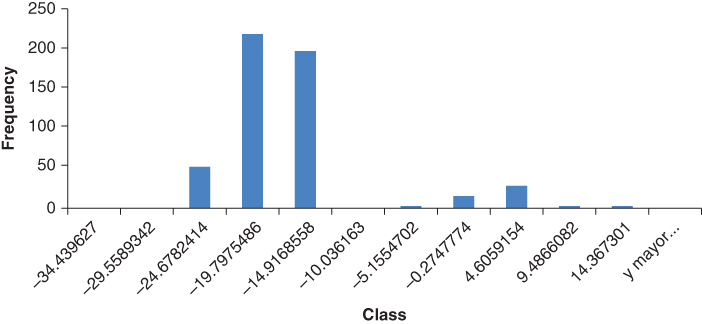
Figure 18.6 Histogram of angle differences between Pascuales and Molino buses for high hydrological scenarios.
Table 18.1 Alert and alarm limits for SNI buses as regards Molino bus—high hydrological scenarios
| 230 kV Bus | Alert Limit | Alarm Limit |
| Milagro | −15.02° | −20.74° |
| Pascuales | −18.86° | −25.65° |
| Pomasqui | −24.27° | −35.62° |
| Quevedo | −21.61° | −29.68° |
| Santa Rosa | −23.42° | −33.98° |
| Totoras | −11.86° | −18.20° |
| Zhoray | −0.98° | −2.16° |
18.4 Steady-State Voltage Stability
Voltage stability refers to the ability of a power system to maintain steady voltages in all buses in the system after being subjected to a disturbance from a given initial operating condition [5]. Computation of Power–Voltage (P-V) curves and the corresponding available transfer capability are the tools most commonly used to analyze the power system steady-state voltage stability [7]. The emerging synchronized phasor measurement technology has allowed the development of novel methodologies to monitor the power system voltage stability in real time. One of the most promising techniques is the so-called Thevenin equivalent method, which allows computing the proximity of the actual operational state to the voltage collapse via the determination of the P-V curve in real time. This tool is mainly being used for monitoring the voltage stability of transmission corridors since it allows determination of the power system relative strength in regards to the load buses [7]. This type of application is offered by WAProtector.
Nevertheless, one of the main challenges is to determine the adequate reference early-warning indicators that allow configuring the real time monitoring application. In this connection, a methodology for determining the voltage profile power transfer limits of the monitored transmission corridors is proposed. These transfer limits are the referential framework for assessing voltage stability in real time, and constitute the early-warning indicators for the system operators. The Thevenin equivalent method allows estimating, in real time, the P-V curve of transmission corridors whose sending bus (B1) and receiving bus (B2) have PMUs installed. Figure 18.7 illustrates a transmission corridor monitored by PMUs.
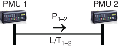
Figure 18.7 Transmission corridor monitored by PMUs.
The receiving end is considered as a load bus (![]() ), which can be calculated with the voltage and current phasor measurements obtained from PMU 2. This end is connected to a Thevenin equivalent consisting of an equivalent voltage generator (
), which can be calculated with the voltage and current phasor measurements obtained from PMU 2. This end is connected to a Thevenin equivalent consisting of an equivalent voltage generator (![]() ) in series with an equivalent impedance (
) in series with an equivalent impedance (![]() ). Based on this approach, the transmission corridor of Figure 18.7 can be represented by the Thevenin equivalent depicted in Figure 18.8.
). Based on this approach, the transmission corridor of Figure 18.7 can be represented by the Thevenin equivalent depicted in Figure 18.8.
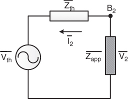
Figure 18.8 Thevenin equivalent of a transmission corridor.
Each parameter of the Thevenin equivalent can be easily determined by using the phasor measurements of PMU 1 and PMU 2, as shown by (18.4) and (18.5) [7]:
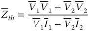
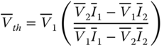
where ![]() and
and ![]() are the voltage and current phasors measured at PMU 1 (sending end), and
are the voltage and current phasors measured at PMU 1 (sending end), and ![]() and
and ![]() are the voltage and current phasors measured at PMU 2 (receiving end).
are the voltage and current phasors measured at PMU 2 (receiving end).
By using the Thevenin equivalent parameters and the computed receiving end load power (i.e., the transfer power), it is possible to determine V2 (voltage magnitude of receiving end) as a function of the transfer power, as shown by (18.6) [7]:
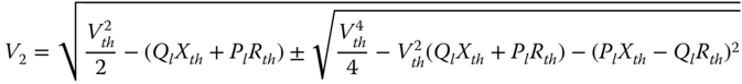
where Pl and Ql are the load's active and reactive power, Rth and Xth are the real and imaginary parts of the Thevenin equivalent impedance (i.e., equivalent resistance and reactance), and Vth is the magnitude of the Thevenin equivalent voltage.
The expression (18.6) constitutes the mathematical representation of the P-V curve of the transmission corridor determined via the Thevenin equivalent method. This curve can be easily determined using real time measurements of voltage and current phasors of PMUs installed at each end of the corridor. WAProtector has an application that computes, in real time, the P-V curve of transmission corridors using the Thevenin equivalent method. Similarly to the steady-state angle stability application, this voltage stability function requires the adequate setting of predefined alert and alarm thresholds, which will give the operators an early-warning signal. These security limits correspond to the so-called voltage profile stability transfer limits, which are determined by applying the existing relationship between P-V curves and the voltage profile stability band, as stated in [8].
Figure 18.9 illustrates a transmission corridor P-V curve obtained via the Thevenin equivalent method in combination with the voltage profile stability band (shaded area). This voltage profile stability band is formed by the upper and lower limits of voltage values for normal voltage operation. The voltage profile stability transfer limit is then calculated considering the first intersection of the P-V curve with the stability band [8], that is, point A in Figure 18.9. For SNI, two bands have been defined based on the concept of normal (−3%) and emergency (−6%) operation [7]. Thus, the alert and alarm threshold values are the result of the P-V curve intersection with the normal and emergency bands, respectively (i.e., normal and emergency voltage profile stability transfer limits).
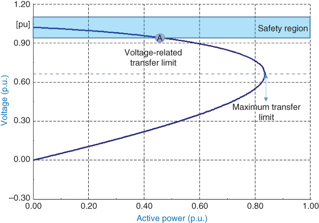
Figure 18.9 P-V curve and voltage profile stability band.
In order to iteratively consider the most critical power transfer conditions in the SNI, taking into account the potential occurrence of N-1 contingencies as well as high and low hydrological scenarios, the methodology depicted in Figure 18.10 has also been included into DIgSILENT PowerFactory via DPL programing scripts. All the formulation of the Thevenin equivalent method has been included in the DPL script in order to compute P-V curves for multiple scenarios. Interested readers can find further explanation of this methodology in [7].
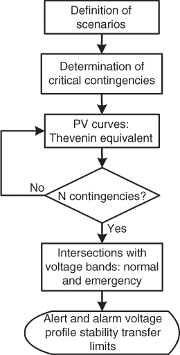
Figure 18.10 Methodology for determining the voltage profile stability transfer limit of transmission corridors.
As an illustration, the P-V curves of the double circuit Totoras–Santa Rosa 230 kV transmission line, per circuit and per unit based on 300 MW, considering maximum load and a high hydrological scenario, are presented in Figure 18.11. The continuous P-V curve corresponds to a normal condition scenario whereas the dotted P-V curve results from the worst voltage-related contingency. The intersections of the worst contingency P-V curve (dotted) with the lower limits of the bands (i.e. −3% and −6%) correspond to the alert and alarm voltage profile stability transfer limits, respectively.
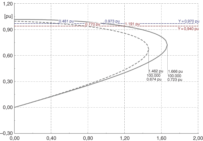
Figure 18.11 P-V curves of the Totoras–Santa Rosa 230 kV transmission line.
With the objective of getting the most representative values of alert and alarm transfer limits, the means of the values obtained for each hydrological scenario are computed. Table 18.2 presents a summary of the alert and alarm limits (mean values) for the Totoras–Santa Rosa 230 kV transmission line considering both high and low hydrological scenarios.
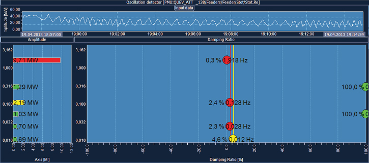
Figure 18.12 Oscillatory event recorded by WAProtector.
18.5 Oscillatory Stability
The rotor angle stability problem involves the study of the electromechanical oscillations inherent in power systems. Oscillatory instability occurs when there is lack of damping torque [5]. Oscillation problems may be either local or global in nature [9]. Local problems (local mode oscillations) are associated with oscillations among the rotors of a few generators close to each other. These oscillations have frequencies in the range of 0.7 to 2.0 Hz. Global problems (inter-area mode oscillations) are caused by interactions among large groups of generators. These oscillations have frequencies in the range of 0.1 to 0.7 Hz. There is another type of oscillatory problem caused by controllers of different system components, named control modes [9]. These types of oscillations present a large associated range of frequencies. From these types of modes, the Ecuadorian National Interconnected System presents the so-called very low frequency control modes (in the range of 0.01 to 0.1 Hz), which usually appear in systems with high penetration of hydroelectric plants and are associated with improper tuning of hydroelectric unit governors.
It is well-known that the damping ratio associated with system dominant modes can vary significantly depending on different factors, such as, for instance, grid strength, generator operating points, loading conditions, and the number of power transfers. Thus, continuous evaluation of the system's damping performance should be performed in order to capture the operating conditions that could entail major damping concerns. In this connection, WAProtector possesses a modal identification algorithm that allows the identification of critical oscillatory modes from the PMUs power flow measurements. This tool allows estimation of the frequency, damping, magnitude, and phase of the critical modes that are observable in a given power flow signal record. The real time data analysis functionality of WAProtector is also complemented by the option of obtaining hourly statistical information of the most predominant oscillatory modes detected by each PMU in order to perform post-operative analysis. Figure 18.12 shows WAProtector's oscillatory application for the active power signal recorded in the PMU installed at Quevedo substation after the outage of the Quevedo–San Gregorio 230 kV transmission line. After this event, power oscillations of large amplitude were recorded, while the transmission line was out of service.
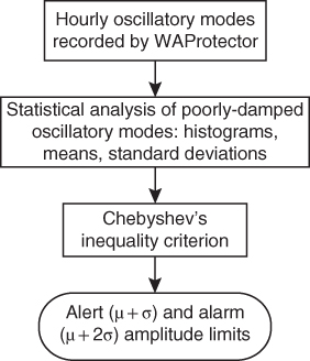
Figure 18.13 Methodology for determining amplitude oscillation limits.
By using the modal identification algorithm, the active power signal immersed modes are determined during the event period, showing the appearance of a local mode at a frequency of 1.918 Hz, damping of 0.3% and a large amplitude of about 9.71 MW. Therefore, this event caused a sustained oscillatory phenomenon that was alerted to the operators via the WAMS application. WAProtector also allows calculating the damping hourly average of dominant oscillatory modes, according to frequency ranges. For this purpose, the modal identification algorithm permanently updates the required windows and calculations, which are recorded in the appropriate databases. It is worth mentioning that the modal identification algorithm of WAProtector constantly regulates itself in order to determine the modes presented in the power signal in the range of 0 to 10 Hz. Through the methodology depicted in the flowchart presented in Figure 18.13, initially introduced by the authors in [10], a statistical analysis of the information obtained from the recorded data of the PMUs located in the power system is performed in order to characterize the oscillatory behavior of the SNI and to determine the most typical amplitudes of oscillations (used to define the alert and alarm amplitude limits).
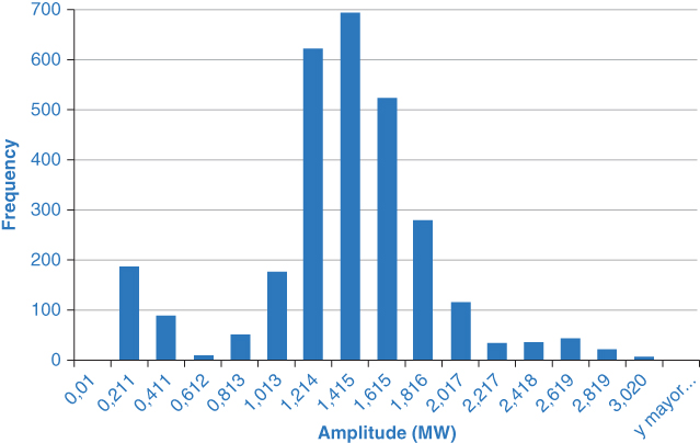
Figure 18.14 Histogram of inter-area mode amplitude.
From the complete information, only modes that present a damping lower than the predefined alert and alarm thresholds are analyzed. These thresholds have been agreed as 5% (alert limit) and 3% (alarm limit) according to the SNI small signal stability periodical study [10]. The proposal corresponds to a statistical analysis carried out via histograms and computation of means and standard deviations of the modes. As an example, Figure 18.14 presents a histogram of the amplitudes of the modes with a damping smaller than 5%, registered within one month.
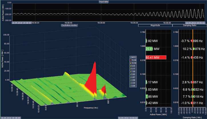
Figure 18.15 Presence of the inter-area mode in the Ecuador–Colombia interconnected system.
This statistical information of oscillatory modes is then employed to determine the limits of oscillation amplitudes that will be used as an early-warning reference for real time monitoring as the alert and alarm settled thresholds. With the statistical information, the alert and alarm limits of amplitudes are determined based on the mean (μ), standard deviation (σ), and the above mentioned Chebyshev's inequality criterion [6], which specifies that at least 50% of the analyzed values should be in the range of one standard deviation around the mean (![]() ), while 75% of the analyzed values should be within the range covered by two standard deviations (
), while 75% of the analyzed values should be within the range covered by two standard deviations (![]() . In this context, the values presented in Table 18.3 have been determined as the alert and alarm limits for the magnitude of the SNI registered oscillations, for the low frequency control modes, inter-area modes, and local modes.
. In this context, the values presented in Table 18.3 have been determined as the alert and alarm limits for the magnitude of the SNI registered oscillations, for the low frequency control modes, inter-area modes, and local modes.
Table 18.2 Alert and alarm voltage limits of Totoras–Santa Rosa 230 kV transmission line per circuit
| High hydrology | Low hydrology | |
| Alert limit (MW) | 254.4 | 149.4 |
| Alarm limit (MW) | 340.8 | 200.1 |
Table 18.3 Alert and alarm amplitude limits for SNI oscillatory modes
| Control modes | Inter-area modes | Local modes | |
| Alert limit (MW) | 2.5 | 1.8 | 0.4 |
| Alarm limit (MW) | 3.5 | 2.4 | 0.6 |
18.5.1 Power System Stabilizer Tuning
As was previously mentioned, the Ecuadorian SNI maintains a permanent 60 Hz synchronous connection with the Colombian power system through four 230 kV transmission lines. It is to be considered that due to voltage control tactics, some of these transmission lines are disconnected in low demand scenarios, increasing the impedance in the connection between the two countries. Several offline analyses and constant monitoring of the oscillatory stability of the Ecuador–Colombia interconnected power system, via the Ecuadorian WAMS, have shown that there is a permanent presence of a poorly damped inter-area mode whose frequency varies within the range of 0.4 to 0.5 Hz. To be more accurate, this mode is mostly seen around a frequency of 0.45 Hz. Figure 18.15 shows the damping and the amplitude of this inter-area mode from WAProtector's Oscillatory Stability tool, as registered by the PMU connected closest to the Colombian system, during a severe event in the SNI. For didactic purposes, the Ecuadorian 230 kV transmission corridor and its connection to Colombia is presented in Figure 18.16.
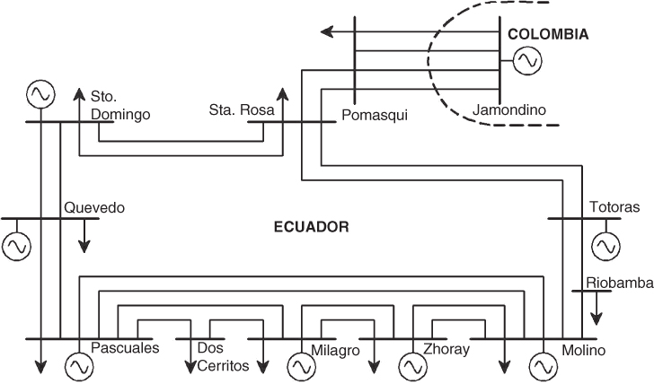
Figure 18.16 Diagram of the 230 kV Ecuadorian transmission corridors.
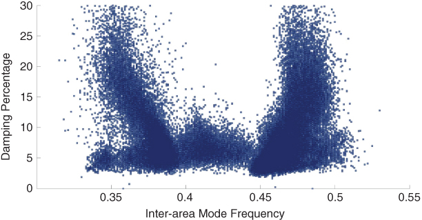
Figure 18.17 Scatter plot of the frequency and damping percentage of the inter-area modes observed in 2015.
It is known that the damping of inter-area modes declines with an increase in the congestion of transmission lines, and consequently with an increase in the angle difference between areas. In this regard, in order to avoid unstable oscillatory conditions in the Ecuadorian system, in some scenarios it has been necessary to limit the power transfer between Colombia and Ecuador, particularly from Ecuador to Colombia, and to avoid disconnecting the interconnection transmission lines. It is easy to see then that improving the damping of the 0.45 Hz inter-area mode will benefit the operation of the Ecuadorian SNI both technically and economically. In order to understand the criticality of the problem, a scatter plot of the frequency and damping of all inter-area modes that appeared during 2015 is presented in Figure 18.17; this has been extracted from the PMUs' available data via the application of the modal identification algorithm of WAProtector. As was previously mentioned for the Ecuadorian system, a mode is considered poorly damped when its damping percentage is smaller than 5%. It is possible to observe that there are two different inter-area modes in the Ecuador–Colombia interconnected power system. One of them corresponds to the 0.45 Hz inter-area mode, which involves the participation of generation units in Colombia and in Ecuador, and the other one whose frequency oscillates between 0.35 and 0.4 Hz involves the action of generators connected in the Ecuadorian system alone.
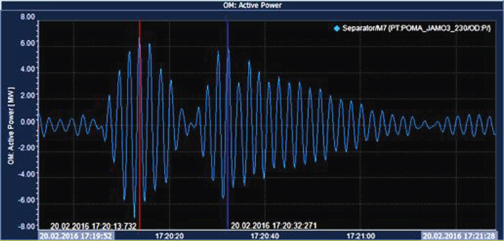
Figure 18.18 Oscillations in the Ecuadorian power system caused by a loss of generation event.
As stated, in order to improve the oscillatory stability in the Ecuador–Colombia interconnected power system, which will ultimately allow increasing the power transfer between these countries, a PSS tuning is done with focus on the 0.45 Hz inter-area mode. According to [12], the phase of oscillations detected in different parts of a system show the differences in the damping contribution from different generators. Thus, generators with leading phase provide less damping to the oscillation mode, while generators with lagging phase provide more damping. In this context, through a phase analysis of signals registered in different PMUs connected in the Ecuadorian power system decomposed in different frequency ranges using the WAProtector modal identification algorithm, it is possible to determine where the 0.45 Hz is more observable, and which generators present a larger participation in this mode—in other words, it is possible to establish the oscillation source location. To illustrate this procedure, Figure 18.18 presents an oscillation detected in the Pomasqui substation. In this particular case, the 0.45 Hz inter-area mode is excited due to a response of the Paute generation plant to a loss of generation event in the Ecuadorian system. The phase analysis of this oscillation using the modal identification algorithm is presented in Figure 18.19. Through the phase analysis, it is possible to determine that, as the inter-area mode was excited, the signals observed in Pomasqui (the closest substation to Colombia), Santa Rosa, and Molino present the highest phase lead; and the signal in Quevedo, a substation not included in the path of the Ecuador–Colombia inter-area mode, presents a phase lag, therefore there are no oscillation sources located in this area. It is then possible to conclude that generators in Colombia and Paute hydroelectric power plant are the biggest contributors to the 0.45 Hz inter-area mode. Paute is one of the largest generation plants in Ecuador and consists of two plants: plant AB connected to the Molino 138 kV substation and plant C connected to the Molino 230 kV bus.
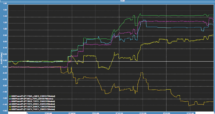
Figure 18.19 Phase analysis of the angle of signals obtained from PMUs.
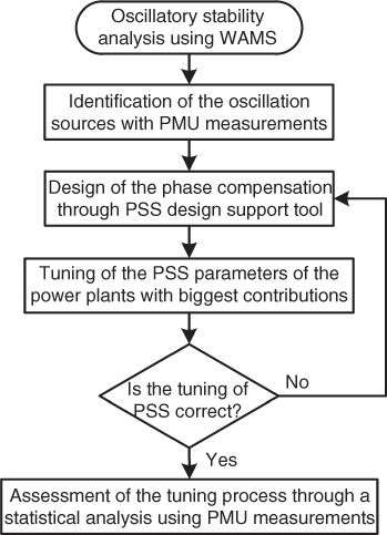
Figure 18.20 Procedure for tuning Paute plant AB stabilizers.
Once it had been determined that the Paute generation plant presents the largest contribution to the 0.45 Hz inter-area mode, from the Ecuadorian side, and considering some technological limitations regarding the structure of the PSSs installed in phase C and the fact that these devices were tuned to improve the damping of a local mode inherent to the plant, a tuning process was carried out for the existing PSSs in phase AB. It is worth mentioning that within this plant, only unit U2 has a digital excitation system. In general terms, Figure 18.20 presents the methodology for carrying out the PSS tuning of the Paute plant's AB generators based on synchrophasor measurements, which also includes the previously presented step.
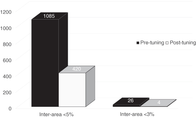
Figure 18.21 Bar plot comparing the appearances of the 0.45 Hz inter-area mode pre-tuning and post-tuning.
For theoretically tuning the power stabilizers in the Paute AB generation plant, the Generator Exciter Power System (GEP) approach was used along with the Single Machine Infinite Bus methodology [13]. The PSS installed in Paute's unit U2 resembles a PSS2B standard, a dual input PSS that is capable of using both generator speed and power, however the speed input was disabled since Ecuador is prone to large frequency deviations due to the predominantly hydro generation and relatively low inertia of the power system [14]. The phase compensation parameters were determined to provide a phase shift in PSS+AVR+Gen as close to −90° as possible, for the main mode frequency, and the washout filter parameters were defined to reduce the low frequency modes and to allow full observability of the 0.4–0.5 Hz inter-area mode.
It is to be noted that the washout transfer function also introduces a phase lead that needs to be accounted for in the design of the phase compensation [13]. Once the parameters were computed, a complete set of field tests using real time information from PMUs connected to each generation unit in Paute was carried out. The gain of the PSS was set based on online tests in order to avoid instability of control modes that would become less stable as the gain is increased. Theoretically, once the instability gain is found, it is reduced to 1/3 of this value [15]. It should be mentioned that during the tuning exercise it was not possible to find control mode instability; therefore the gain was limited not by control stability issues, but rather by the allowable MVAr swings in the generation unit [14].
Once the PSS tuning of the Paute AB generation plant was concluded, it was necessary to carry out a monitoring stage in order to identify the effectiveness of the process. For this purpose, the same WAProtector modal identification algorithm was used in order to determine the damping of the inter-area mode before and after the tuning, considering a one month test period. It is possible to determine that the tuning of the PSSs of the Paute AB generation plant had a positive effect on damping the 0.45 Hz inter-area mode, as can be seen in the bar plot presented in Figure 18.21. From this data, it has been determined that the number of appearances of this mode with a damping percentage below 5% has decreased by about 61%.
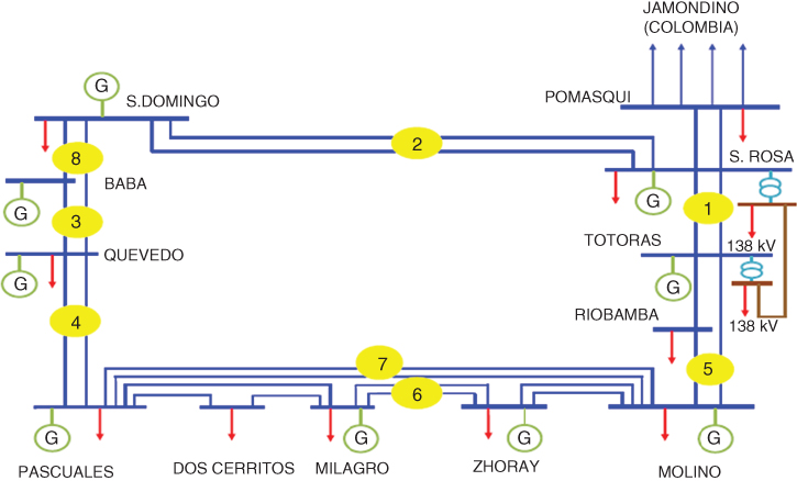
Figure 18.22 Diagram of the implemented strategies in the SPS.
Interested readers can find further explanation of this methodology in [16].
18.6 Ecuadorian Special Protection Scheme (SPS)
Special Protection Schemes (SPS) are designed in order to detect abnormal conditions and carry out corrective actions that mitigate possible consequences and allow an acceptable system performance. However, the conditions that lead the system to blackouts are not easy to identify mainly because the process of system collapse depends on multiple interactions. In this connection, some Smart Grid applications have been designed in order to perform timely self-healing and adaptive reconfiguration actions based on system-wide analysis, with the objective of reducing the risk of power system blackouts. Real time dynamic vulnerability assessment (DVA) has to be done first in order to decide and coordinate the appropriate corrective control actions, depending on the event evolution. Emerging technologies such as PMUs and WAMS offer a new benchmark for performing post-contingency DVA that could be used to trigger SPSs in order to implement enhanced corrective control actions [17].
In the Ecuadorian case, ensuring efficiency in the daily operation of the SNI has become a paramount concern due to several factors that have increased the potential sources for system disturbances and occasionally lowered the operational security and flexibility. Among these factors are weakly meshed topology and unsymmetrical distribution of generation and load, especially for distant portions of the eastern and southern areas that are radially connected to the main 230 kV transmission ring [18, 19]. Component failures and protections operation due to bottlenecks in key transmission corridors have sometimes led to adverse consequences such as partial or widespread disruptions. Occasionally, overloading of certain transmission facilities occur, especially due to high power transfers from bulk generation located in the central and southern areas to the main consumption centers in the northern (i.e., Quito) and southwestern (i.e., Guayaquil) areas; this can entail congestion, unexpected generation outages, load shedding, and/or poor dynamic performance. In this connection, the Special Protection Scheme (SPS) portrayed in this section was designed to prevent out-of-step conditions between Ecuador and Colombia or the separation of both grids, which can lead to a grid collapse in Ecuador. The study results, based on different operational scenarios that consider double contingencies of the 230 kV main trunk transmission lines, and subsequent statistical and regression analyses, have led to the establishment of tables of mitigation actions that must present a quick response (less than 200 ms) in real time to predefined contingencies. These tables represent functions that allow determination of the place where the contingency occurs and the loads that are in the affected and nearby circuits, in order to execute adequate countermeasures. The mitigation actions comprise the automatic shedding of computed quantities of generation and load at pre-specified locations or regions. The Ecuadorian SPS is defined as an automatic system, composed of a set of elements of protection, control, and communication networks, which acts upon the occurrence of predefined events (the untimely disconnection of critical SNI branches), executing a post-contingency corrective action composed of calculated load shedding and disconnection of generation, in order to avoid or mitigate problems of instability. The SPS is a wide area controller of stability of a power system that is capable of responding in a very short time (in the order of milliseconds) [20]. The Ecuadorian SPS is based on synchrophasor technology that makes up a redundant control scheme made up by 58 local relays with built-in PMU functionality installed in the main SNI substations. Inside the so-called Mitigation Matrix there is a set of equations, for each of the strategies listed in Table 18.4 and represented in Figure 18.22, that allows calculating the right amount of load and generation that must be disconnected in order to avoid system instability, on occurrence of one of the eight defined N-2 contingencies, taking into account the pre-fault power flow in the transmission corridors. The reader can find further information about the SPS implemented in Ecuador in [21].
Table 18.4 Implemented strategies in the SPS
| Strategy | N-2 Transmission lines contingencies |
| 1 | Santa Rosa–Totoras |
| 2 | Santo Domingo–Santa Rosa |
| 3 | Santo Domingo–Quevedo and Quevedo–Baba |
| 4 | Quevedo–Pascuales |
| 5 | Totoras–Molino and Molino–Riobamba |
| 6 | Milagro–Zhoray |
| 7 | Molino–Pascuales |
| 8 | Santo Domingo–Quevedo and Santo Domingo–Baba |
18.6.1 SPS Operation Analysis
On May 6, 2015, the Molino–Pascuales 230 kV transmission line got disconnected (strategy 7) with a pre-fault power flow of 414 MW. According to the analysis performed, the strategy programmed in the SPS for this contingency should be activated with a power flow of 350 MW. In accordance with the expressions defined for this strategy, as depicted in (18.7) and (18.8), the execution of the mitigation actions produced the disconnection of 114 MW of generation and 123 MW of load, causing around 89.2 MWh of energy not supplied. It is worth mentioning that it only took 141.7 ms, after the detection of the switching of the transmission line, for the SPS to execute all mitigation actions.
where DP and DPLoad are the active power values that need to be disconnected from generators and loads, respectively, P is the measured pre-fault power flow through the transmission line, DPactual is the real disconnected amount from generation, and k7_1, k7_2, Pset7_2 and Pset7_3 are the previously defined constants via the above mentioned regression analysis. These computations are done inside a master smart PDC that manages the local relays.
In order to evaluate the effectiveness of the SPS, a post-mortem analysis was performed via simulation to estimate the consequences in the SNI operation in the face of the occurrence of this contingency without the SPS. It was possible to determine that after the contingency of the Molino–Pascuales 230 kV transmission line, there would have been a large reactive power requirement in the Guayaquil area, mainly caused by the loss of the reactive compensation supplied by Paute generation plant and by the reactive power consumption of nearby transmission lines due to the sudden increase of the active power. This reactive power deficit would have certainly caused the switching of two major generation plants in the Guayaquil area due to over-excitation and thus a further reactive power deficit and subsequent uncontrollable voltage decay. In this context, it is possible to establish that without the SPS, the outage of the Molino–Pascuales transmission line would have caused a voltage collapse in several SNI substations. From the available data it was determined that this voltage collapse would have caused the outage of about 893.4 MW of load. In raw numbers, and assuming the feasibility of restoring the power supply to the affected areas in approximately 1 or 1.5 hours, the energy not supplied would have reached an estimated value between 893 MWh and 1340 MWh. In Ecuador, the cost of energy not supplied is 1533.00 USD/MWh (defined by the Regulator), and so, as shown in Table 18.5, the actuation of the SPS was able to prevent the loss of an economic amount between USD 1.2 million and USD 1.9 million, in one event alone.
Table 18.5 Energy Not Supplied cost with and without the actuation of SPS
| Energy not supplied (MWh) | Cost from energy not supplied (USD MM) | |
| Without SPS | [893.4, 1340.1] | [1.37, 2.05] |
| With SPS | 89.2 | 0.14 |
| Economic savings | [1.2, 1.9] |
18.7 Concluding Remarks
Three methodologies for determining adequate thresholds regarding: (i) phase angle difference, (ii) voltage profile power transfer of transmission corridors, and (iii) oscillatory issues have been presented in this chapter. These limits are calculated periodically and are later set into the WAProtector application as the referential framework for assessing stability in real time. Additionally, a practical procedure for determining the source locations of poorly damped low frequency power system oscillations using WAMS records was presented. For this purpose, the WAProtector's modal identification algorithm was used in order to determine the Ecuadorian system oscillatory behavior. Afterwards, the tuning of PSSs and further assessment was also carried out based on the results obtained from the WAMS application. It is feasible to determine that the PSS tuning process performed in the Ecuadorian SNI, whose main focus was to improve the damping of the Ecuador–Colombia inter-area mode, had successful results, considering the decrease in the appearances of poorly damped 0.45 Hz inter-area modes. A similar procedure will be followed for tuning additional PSSs in the Ecuadorian system with the aid of a real time digital simulator recently implemented in CENACE.
The Ecuadorian Special Protection Scheme (SPS) was designed to prevent partial or total collapses in the SNI due to the occurrence of eight defined double contingencies in the 230 kV trunk transmission corridors. Since its commissioning, it has had three satisfactory actuations and it has been established that during the outage of the Molino–Pascuales 230 kV transmission line, the SPS was able to prevent the loss of an economic amount between USD 1.2 million and USD 1.9 million, taking into consideration the cost of energy not supplied (CENS) in Ecuador. Due to the growth of the SNI, the SPS will be redesigned, using also the recently implemented real time digital simulator.
References
- 1 J. Cepeda, J. Rueda, G. Colomé and I. Erlich, “Data-Mining-Based Approach for Predicting the Power System Post-contingency Dynamic Vulnerability Status,” International Transactions on Electrical Energy Systems, vol. 25, issue 10, pp. 2515–2546, October 2015.
- 2 J. Cepeda and P. Verdugo, “Determinación de los Límites de Estabilidad Estática de Ángulo del Sistema Nacional Interconectado,” Revista Técnica “energía”, No. 10, January 2014.
- 3 IEEE Power Engineering Society, “IEEE Standard for Synchrophasors for Power Systems,” IEEE Std. C37.118.12011, December 2011.
- 4 A. De La Torre and J. Cepeda, “Implementación de un sistema de monitoreo de área extendida WAMS en el Sistema Nacional Interconectado del Ecuador SNI,” Ingenius, vol. 10, pp. 34–43, 2013.
- 5 P. Kundur, J. Paserba, V. Ajjarapu, et al, “Definition and Classification of Power System Stability,” IEEE/CIGRE Joint Task Force on Stability: Terms and Definitions. IEEE Transactions on Power Systems, vol. 19, August 2004.
- 6 J. Han and M. Kamber, Data Mining: Concepts and Techniques. Second edition, Elsevier, Morgan Kaufmann Publishers, 2006.
- 7 J. Cepeda, P. Verdugo and G. Argüello, “Monitoreo de la Estabilidad de Voltaje de Corredores de Transmisión en Tiempo Real a partir de Mediciones Sincrofasoriales,” Revista Politécnica, vol. 33.
- 8 Y. Nguegan, Real-time identification and monitoring of the voltage stability margin in electric power transmission systems using synchronized measurements. Universität Kassel, Doctoral Thesis, June 2009.
- 9 P. Kundur, Power System Stability and Control. McGraw-Hill, Inc., Copyright 1994.
- 10 J. Cepeda, and A. De La Torre, “Monitoreo de las oscilaciones de baja frecuencia del Sistema Nacional Interconectado a partir de los registros en tiempo real,” Revista Técnica “energía”, No. 10, January 2014.
- 11 L. Grigsby, Power system stability and control, Boca Raton: Taylor & Francis Group, 2007.
- 12 N. Al-Ashwal, D. Wilson and M. Parashar, “Identifying Sources of Oscillations Using Wide Area Measurements”, CIGRE US National Committee, 2014.
- 13 D. Wilson, N. Al-Ashwal and K. Hay, “Power System Stabiliser Tuning: Part 1 System Analysis & Plant Selection”, ALSTOM – PSYMETRIX Consulting Project, 2015.
- 14 D. Wilson, N. Al-Ashwal and B. Berry, “Power System Stabiliser Tuning: Part 3 Final Report”, ALSTOM – PSYMETRIX Consulting Project, 2015.
- 15 J. Agee, S. Patterson, R. Beaulieu, M. Coultes, R. Grondin, I. Kamwa, et al., “IEEE tutorial course power system stabilization via excitation control”, IEEE Power and Energy Society, June 2007.
- 16 P. Verdugo, J. Cepeda, A. De La Torre, D. Echeverría, and H. Flores, “Oscillation Source Location and Power System Stabilizer Tuning Using Synchrophasor Measurements”, IEEE Transmission and Distribution Latin America (T&D-LA) 2016, Morelia, México, September 2016.
- 17 J. Cepeda, “Real Time Vulnerability Assessment of Electric Power Systems Using Synchronized Phasor Measurement Technology”, National University of San Juan, Doctoral Thesis, December 2013.
- 18 Corporación Eléctrica del Ecuador-TRANSELECTRIC, “Plan de expansión de transmisión período 2013–2022”, Quito, March 2012.
- 19 Agencia de Regulación y Control del Ecuador-ARCONEL, “Plan Maestro de Electrificación 2013–2022”, Quito, Available: http://www.conelec.gob.ec.
- 20 S. Wang, and G. Rodriguez, “Smart RAS (Remedial Action Scheme)”, Innovative Smart Grid Technologies (ISGT), IEEE, Gaithersburg, MD, 2010.
- 21 M. Flores, D. Echeverría, R. Barba and G. Argüello, “Architecture of a Systemic Protection System for the Interconnected National System of Ecuador”, 2015 Asia-Pacific Conference on Computer Aided System Engineering (APCASE), IEEE, Quito, July 2015.