
CHAPTER 8
Quantitative Momentum Beats the Market
“… we slavishly follow the model. You do whatever it says no matter how smart or dumb you think it is.”
– Jim Simons, Renaissance Technologies1
The components and knowledge required to understand the quantitative momentum system are outlined in Chapters 5 through 7. In Chapter 5, we outline the generic relative strength momentum indicator commonly used in academic research. Generic momentum is a starting point in the quantitative momentum system. We calculate the generic momentum measure as the total return (including dividends) of a stock over some particular look-back period (e.g., the past 12 months) and skip the most recent month. We calculate this measure for all stocks in our investment universe.
The next aspect of the quantitative momentum system relates to how we differentiate among generic momentum stocks. If you recall, in Chapter 6 we speak to the evidence on two aspects of investor behavior: (1) a preference for lottery-like assets and (2) limited attention. We first show the evidence that stocks with large short-term “spikes” in performance generally underperform. This underperformance is the result of mispricing caused by biased investors who overpay for lottery-like stock characteristics. Next, we examine the so-called frog-in-the-pan momentum algorithm (FIP), which attempts to quantify the path of a high momentum stock. The calculation for the measure is described as follows:
The FIP measure looks at the past 252 trading days for all high-momentum stocks and tabulates the percentage of trading days with negative returns and the percentage of trading days that are positive. These two calculation components are subtracted from one another and multiplied by the sign of the generic momentum signal (i.e., 12-month total return, skipping the first month). For example, say stock ABC has a generic momentum calculation of 50 percent. If 35 percent of the past 252 trading days are negative, 1 percent of trading days are flat, and 64 percent are positive, then ABC's ![]() . The more negative the FIP, the better. The FIP algorithm separates high momentum stocks into those that have more continuous price paths (i.e., smooth, with a slow diffusion of gradual information elements) versus those high momentum stocks that have more discrete price paths (i.e., jumpy, with immediate information elements). The FIP algorithm serves as a 2-for-1 benefit, as it systematically minimizes exposure to lottery-like stock characteristics and focuses on those high momentum stocks that are most likely to be suffering from the core reason why momentum stocks outperform: investors are systematically underreacting to positive news.
. The more negative the FIP, the better. The FIP algorithm separates high momentum stocks into those that have more continuous price paths (i.e., smooth, with a slow diffusion of gradual information elements) versus those high momentum stocks that have more discrete price paths (i.e., jumpy, with immediate information elements). The FIP algorithm serves as a 2-for-1 benefit, as it systematically minimizes exposure to lottery-like stock characteristics and focuses on those high momentum stocks that are most likely to be suffering from the core reason why momentum stocks outperform: investors are systematically underreacting to positive news.
Finally, in Chapter 7, we investigate seasonality and how it relates to momentum strategies. The core finding from this chapter is that window dressing and tax minimization incentives likely play a role in the time series dynamics of the profitability of momentum strategies. We discuss the difficulty of exploiting this seasonality evidence due to real-world concerns related to frictional costs and trading complexity. However, we highlight that this information can be indirectly leveraged by incorporating seasonality knowledge into the rebalance program of a momentum strategy. Our research highlights that timing momentum strategy rebalances, such that the strategy trades ahead of window dressers and tax motivated investors, delivers a positive contribution to expected performance.
In the end, we boiled down our momentum process into five sequential steps (depicted in Figure 8.1):

Figure 8.1 Quantitative Momentum Process
- 1. Identify Investable Universe: Our universe generally consists of mid- to large-capitalization U.S. exchange-traded stocks.
- 2. Generic Momentum Screen: We rank stocks within our universe based on their past 12-month returns, ignoring the last month.
- 3. Momentum Quality Screen: We screen high-momentum stocks on the “quality” of their momentum, which we measure via the FIP algorithm.
- 4. Momentum Seasonality Screen: We take advantage of seasonal aspects applicable to momentum investing, which determines the timing of our rebalance. We rebalance quarterly before quarter ending months.
- 5. Invest with Conviction: We seek to invest in a concentrated portfolio of stocks with the highest quality momentum. This form of investing requires disciplined commitment, as well as a willingness to deviate from standard benchmarks.
A hypothetical portfolio construction scenario would work in the following way. Consider a universe of 1,000 stocks identified in step 1. In step 2, we calculate generic momentum scores for each of the 1,000 securities and identify the top 10 percent, or 100 highest generic momentum stocks. For step 3, we calculate the FIP score for the 100 high-momentum names identified in step 2 and rank these 100 stocks on FIP, where lower is better. We identify the top half, or 50 high-momentum stocks with the smoothest momentum. In step 4, we determine the model portfolio and conduct our rebalance at the end of February, May, August, and November to exploit seasonality effects. Finally, in step 5, we implement the roughly 50-stock portfolio strategy with an equal-weight construction (to minimize stock specific risk) and prepare for high relative performance volatility and the blessing (and curse) of long periods of relative outperformance (and underperformance).
TRANSACTION COSTS
Transaction costs are commonly discussed as a core reason why momentum is a failed investment practice left to the hypothetical day trading technical analysis heretics who lack brains. We covered some of the academic research on the subject of momentum profits net of transaction costs in Chapter 5. And while the academic research consensus is that transaction costs matter for momentum strategies, as they do for any active investment strategy, the myth of momentum strategies as being too expensive to exploit is probably too strong. This “myth” is often preached by those who are (1) unfamiliar with the research on the subject and (2) have never had experience trading momentum strategies in practice. Cliff Asness et al. attack this issue head on in their appropriately titled paper “Facts, Fiction, and Momentum Investing.” Asness states succinctly that “you don't have to do much math to realize that momentum can easily survive trading costs.”2 We encourage interested readers to explore and compare the analysis of momentum transaction costs presented in Frazzini, Israel, and Moskowitz,3 who analyze realized transaction costs data from AQR capital over a sustained period of time, and Lesmond, Schill, and Zhou, who estimate trading costs from daily and intra-day analysis via an academic exercise that does not consider that professional investors have much lower trading costs and implement strategies to minimize rebalance costs.4 Of course, extrapolating Asness's research too far would also be foolish. Common sense suggests that one cannot jam billions upon billions of dollars into momentum strategies without recourse. If more disciplined capital is deployed into momentum strategies over time, without a corresponding decrease in transaction costs, the net benefit to a momentum strategy may become muted.
When testing the quantitative momentum algorithm, we must decide at the outset of the investment simulation how we incorporate transaction costs into our backtests. For simplicity, we incorporate a 1 percent management fee, under the assumption that most investors would need to hire a professional to implement a robust momentum strategy, and a 0.20 percent rebalancing cost. Our 0.20 rebalance cost is assessed four times per year for a quarterly rebalanced strategy, and this translates into a 0.80 percent annual trading cost. The total management fee and trading costs sum up to 1.80 percent per year, which is what we use for all the analysis we present in this chapter, unless stated otherwise.
Now, before the reader suffers a knee-jerk reaction that the fees should be much higher or much lower, consider the fact that we already know this estimate is unlikely to be the true estimate and will vary wildly. In practice, different investors will have different cost structures, tax situations, and trading and execution skills. Cost assumptions for one group of investors can be a degree of magnitude larger (or smaller) for another set of investors. We are merely establishing a baseline cost estimate to take into account the fact that costs will have some effect on the final outcome. In our own live trading of the quantitative momentum strategy, we have experienced much lower trading costs than those assumed, but historically the trading costs would have been much higher than those assumed. We hope that our estimate is a “goldilocks” estimate—not too cold; not too hot; and perhaps just right. We don't claim to have the perfect answers and we encourage all investors to gauge the expected costs of running these systems and adjust the results accordingly.
THE PARAMETERS OF THE UNIVERSE
To ensure other researchers have enough information to replicate and independently verify our results, we outline the details of the stock universe we explore and the assumptions we make to conduct our analysis in Table 8.1. Our universe is liquid and investable, requiring a minimum market capitalization at each rebalance period that is greater than the NYSE 40 percent market capitalization breakpoint at the time of the rebalance. Our analysis runs from March 1, 1927, through December 31, 2014,5 and our data come from the academic research gold standard for return data: CRSP (The Center for Research in Security Prices).
Table 8.1 Universe Selection Parameters
| Item | Item Description |
| Market Capitalization | NYSE 40% Breakpoint |
| Exchanges | NYSE/AMEX/NASDAQ |
| Included Security Types | Ordinary Common Shares |
| Excluded Industries | None |
| Return Data | Prices adjusted for dividends, splits, and corporate actions |
| Delisting Algorithm | “Delisting Returns and their Effect on Accounting-Based Market Anomalies,” by William Beaver, Maureen McNichols, and Richard Price6 |
| Portfolio Weights | Market-capitalization weighted (VW, or value-weight) |
QUANTITATIVE MOMENTUM ANALYSIS
We do a deep dive into the historical performance of the quantitative momentum system. Our analysis is organized as follows:
- Summary statistics
- Reward analysis
- Risk analysis
- Robustness analysis
Summary Statistics
Table 8.2 sets out the standard statistical analyses of the quantitative momentum strategy's performance and risk profile, comparing it to the generic momentum strategy (no seasonality, no FIP), and the Standard & Poor's 500 Total Return Index (S&P 500 TR Index). The returns shown in Table 8.2 are net of 1.80 percent in fees for all three of the momentum strategies, and the S&P 500 Index is gross of fees. We give the passive index an unrealistic cost advantage (i.e., free) to ensure we are conservative in our assessment of the results. All results are value-weight (sometimes referred to as market-cap weight) to maintain consistency. An alternative weighting scheme is to equal-weight the portfolio holdings. This alternative equal-weighting scheme is beneficial in two ways:
Table 8.2 VW Quantitative Momentum Performance (1927–2014)
| Quantitative Momentum (Net) | Generic Momentum (Net) | S&P 500 Index | |
| CAGR | 15.80% | 13.45% | 9.92% |
| Standard Deviation | 23.89% | 23.62% | 19.11% |
| Downside Deviation | 17.56% | 17.44% | 14.22% |
| Sharpe Ratio | 0.60 | 0.51 | 0.41 |
| Sortino Ratio (MAR |
0.72 | 0.60 | 0.44 |
| Worst Drawdown | –76.97% | –75.81% | –84.59% |
| Worst Month Return | –31.91% | –30.15% | –28.73% |
| Best Month Return | 31.70% | 33.73% | 41.65% |
| Profitable Months | 63.00% | 61.39% | 61.76% |
- Diversification—You allocate the same percentage of capital to each stock, so no one stock has a large weight in the portfolio.
- Small-cap Effect—On average, the returns to smaller stocks has been larger in the past, and for our portfolio, this means higher expected returns.
Table 8.2 shows that the quantitative momentum strategy generated a compound annual growth rate (CAGR) of 15.80 percent, significantly outperforming the generic momentum performance of 13.45 percent. The Quantitative Momentum strategy also outperformed the S&P 500, which returned 9.92 percent.
The quantitative momentum portfolio achieved this return with a much higher volatility than the benchmark portfolio, which is to be expected because the portfolio is more concentrated than the passive benchmark (i.e., averages 43.9 stocks over the time period) and the strategy is designed to be difficult to follow. Quantitative momentum had a standard deviation of 23.89 percent against the passive S&P 500 benchmark volatility measure of 19.11 percent. Despite the enhanced volatility, the risk-adjusted parameters are still favorable for the quantitative momentum strategy. The strategy has a Sharpe ratio of 0.60, considerably better than the S&P 500 Sharpe ratio of 0.41. The strategy also has a higher downside volatility, with downside deviation at 17.56 percent to the benchmark's 14.22 percent. However, the higher returns compensate for the higher downside volatility, leading to an exceptional Sortino ratio of 0.72 for the quantitative momentum strategy, against 0.44 for the benchmark.
If we look at the worst drawdowns, which represent the worst possible peak-to-trough returns associated with the various strategies, the quantitative momentum strategy showcases that the strategy can be extraordinarily painful! The worst drawdown suffered by the quantitative momentum portfolio is –76.97 percent, which is the Great Depression drawdown (the benchmark drawdown was an even worse –84.59 percent).
We must emphatically emphasize that investors need to be prepared for the enhanced volatility and drawdown risks associated with momentum strategies—that is a primary reason why this system is expected to work in the future—but this enhanced risk is more than offset by additional expected returns, which is what makes momentum anomalous.
Rewards Analysis
Consider Figure 8.2, which shows the cumulative performance of the quantitative momentum portfolio compared to the other strategies.
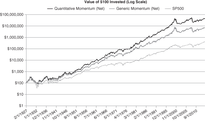
Figure 8.2 Cumulative Value for Quantitative Momentum (1927–2014)
Figure 8.2 illustrates the effects of compounding an edge over a long period of time. The quantitative momentum portfolio's small advantage leads to a jaw-dropping spread relative to the passive benchmark.
Table 8.3 shows the compound annual growth rates (CAGR) of the quantitative momentum portfolio and the competition over different decades. The intent of this test is to examine the robustness of performance across time.
Table 8.3 CAGR Across Different Decades
| Quantitative Momentum (Net) | Generic Momentum (Net) | S&P 500 Index | |
| 1930–1939 | 3.08% | 1.64% | –1.34% |
| 1940–1949 | 11.01% | 11.85% | 9.15% |
| 1950–1959 | 24.98% | 21.31% | 19.42% |
| 1960–1969 | 20.50% | 18.26% | 7.84% |
| 1970–1979 | 13.93% | 13.21% | 5.83% |
| 1980–1989 | 24.48% | 17.38% | 17.61% |
| 1990–1999 | 36.48% | 30.21% | 18.37% |
| 2000–2009 | –3.58% | –4.88% | –0.68% |
Over eight full decades, the quantitative momentum portfolio outperformed in seven of the eight. A concern some may have is that the quantitative momentum portfolio lost in the most recent decade. Perhaps momentum is dead because the smart arbitrageurs eliminated the momentum premium? We can never eliminate this possibility; however, a decade of underperformance is not unexpected. Geczy and Samonov find that long periods of poor relative performance occur on multiple occasions in out-of-sample testing over the 1801 to 1926 time period.7 Moreover, as we explained earlier in the book, sticking to the algorithm is difficult because of the high volatility and career risk. Second, if one examines the net of fee results of the equal-weighted quantitative momentum portfolio (not shown), this portfolio actually outperformed on a CAGR basis over the 2000–2009 decade. Nonetheless, no sustainable system can work all the time. And while Figure 8.2 makes quantitative momentum seem like a “no-brainer,” a deeper dive into shorter windows highlights the fact that there are periods of extreme relative underperformance over the 1927 to 2014 period. Momentum investing is simple, but not easy.
Here we look at a variety of measures to assess the performance across rolling periods. Figures 8.3a and 8.3b show the rolling 5- and 10-year CAGRs for the strategy. These figures show the relevant holding period return at different points in time. A robust strategy will show consistent outperformance regardless of timing; a “lucky” strategy may have extreme outperformance in one time period but flounder in others.

Figure 8.3a Five-Year Rolling CAGR for Quantitative Momentum

Figure 8.3b Ten-Year Rolling CAGR for Quantitative Momentum
Figures 8.3a and 8.3b illustrate how consistently the strategy beats the Generic momentum portfolio and the S&P 500 on rolling 5- and 10-year bases. Only rarely, and for brief periods, was it better to have been invested in the others. Two periods of long-term underperformance include the Great Depression period and the most recent period following the 2008 financial crisis. This underperformance is to be expected, and appreciated, because these periods “shake out” weak hands. Over the long haul, a sustainable process executed with discipline wins out.
Risk Analysis
As the previous analysis emphasizes, the power of momentum is an ability to generate outsize returns that dwarf returns associated with passive benchmarks. Unfortunately, outsized expected returns deliver enhanced risks. The risk and reward trade-off for momentum is still favorable, but not acknowledging the increased risk would be intellectually dishonest and set up a prospective momentum investor with the improper expectations. We examine the risks associated with quantitative momentum in the analysis that follows.
Our risk analysis focuses on maximum drawdowns. The maximum drawdown is defined as the maximum peak to trough loss associated with a time series. Maximum drawdown captures the worst possible performance scenario experienced by a buy and hold investor dedicated to a specific strategy. The intuition behind maximum drawdown is simple: How much can I lose?
Figure 8.4 shows the summary drawdown performance of quantitative momentum across commonly assessed horizons of one month, one year, and three years.

Figure 8.4 Summary Drawdown Analysis
The quantitative momentum strategy protects capital nearly as well as the competition based on the results in Figure 8.4. The strategy's single-worst drawdown was worse than the generic momentum strategy, but beat the S&P 500. However, quantitative momentum did lose over rolling 1- and 12-month periods to the competition. The worst-case scenario for the strategy over a 3-year period was again slightly better than the S&P 500. To be clear—our portfolio is a long-only strategy, so it is expected to have similar drawdowns when compared to the market.
Figures 8.5a and 8.5b show the rolling 5- and 10-year maximum drawdowns for the strategy. These figures help researchers identify the frequency and intensity of a strategy's maximum drawdowns over a designated time horizon (e.g., 5 years or 10 years). But why are rolling drawdowns a useful analytical tool? Consider two strategies with similar worst drawdowns. If one strategy experiences big drawdowns several times through history, while the other experiences big drawdowns only once, this analysis helps us identify this higher frequency of large drawdowns.

Figure 8.5a Five-Year Rolling Max Drawdown for Quantitative Momentum

Figure 8.5b Ten-Year Rolling Max Drawdown for Quantitative Momentum
The rolling drawdown analysis shows that the strategy suffers drawdowns that can be larger than the competition. For example, in the aftermath of the Internet bubble, quantitative momentum took it on the chin, especially compared to the broad index. Similarly, in the 2008 financial crisis, the quantitative momentum portfolio was hit a bit harder than the broad index.
Finally, we end our analysis with an assessment of the relative performance of quantitative momentum during the strategy's worst 10 drawdowns. We compare the quantitative momentum drawdowns to the performance of the passive index over the same time period. This analysis gives us insight into the tail-risk correlations between the quantitative momentum strategy and the passive market. Table 8.4 highlights two points: First, quantitative momentum is a long-only equity strategy with huge drawdowns. Second, the drawdowns are correlated with general market drawdowns. Overall, the quantitative momentum portfolio will have large drawdowns and periods of underperformance, and one should expect this at the outset.
Table 8.4 Top 10 Drawdown Analysis
| Rank | Date Start | Date End | Quantitative Momentum | S&P 500 TR Index |
| 1 | 1/31/1929 | 5/31/1932 | –76.97% | –80.67% |
| 2 | 2/29/2000 | 2/28/2003 | –68.14% | –35.14% |
| 3 | 6/30/2008 | 2/28/2009 | –62.12% | –40.82% |
| 4 | 3/31/1937 | 3/31/1938 | –52.99% | –51.11% |
| 5 | 12/31/1972 | 9/30/1974 | –38.68% | –42.73% |
| 6 | 11/30/1961 | 6/30/1962 | –34.57% | –21.97% |
| 7 | 5/31/1946 | 6/30/1949 | –31.69% | –13.77% |
| 8 | 9/30/1987 | 11/30/1987 | –30.88% | –28.00% |
| 9 | 4/30/1940 | 4/30/1942 | –30.81% | –26.52% |
| 10 | 11/30/1968 | 6/30/1970 | –27.23% | –29.23% |
Robustness Analysis
In this section, we examine a variety of tests that look at a strategy from different angles so that we can gain insight into the big picture and ascertain that the summary statistics reflect a broad reality that is not driven by extreme outliers.
We first analyze market cycle performance of the quantitative momentum strategy compared to the other strategies over a variety of bull and bear markets since 1927. Table 8.5 shows the dates used to calculate market cycle returns.
Table 8.5 Market Cycle Definitions
| Month Begin | Month End | |
| Bear | September-29 | July-32 |
| Bull | June-62 | February-66 |
| Bear | November-68 | May-70 |
| Bull | May-70 | December-72 |
| Bear | January-73 | September-74 |
| Bull | June-82 | December-84 |
| Bear | July-87 | December-87 |
| Bull | December-87 | June-90 |
| Bear | March-00 | September-01 |
| Bull | October-01 | July-07 |
| Bear | August-08 | February-09 |
| Bull | March-09 | December-14 |
Figure 8.6 demonstrates that, on average, the strategy performed similar to the S&P 500 in bear markets and outperformed the S&P 500 in bull markets. Again, relative losses to the S&P 500 appear in the most recent bear and bull markets. There are surely commentators that claim “momentum is dead.” Great, we hope this commentary continues. While the strategy may occasionally struggle for short—or even long—periods of time, momentum systems provide a high chance of expected outperformance through a full market cycle.
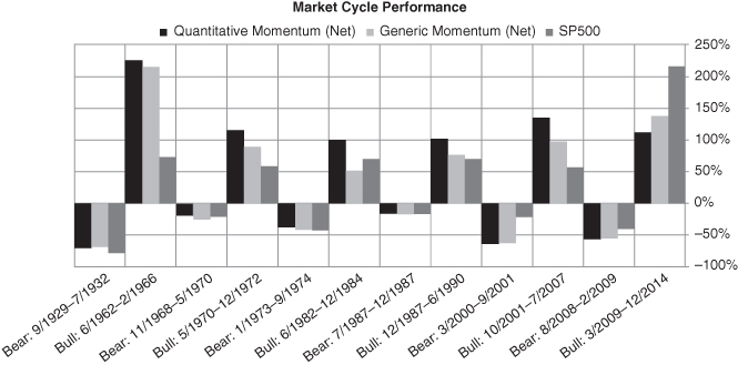
Figure 8.6 Market Cycle Performance for Quantitative Momentum
Figure 8.7 shows the relative performances during recent short-term stress events of the quantitative momentum strategy and the other strategies. This analysis examines how a strategy tends to perform through extraordinary short-term market events. The model shows strong performance compared to the other S&P 500 during the NASDAQ run-up, but underperformance in the NASDAQ crash in 1998 and the 2008 financial crisis.

Figure 8.7 Short-Term Stress Event Tests for Quantitative Momentum
Figures 8.8a and 8.8b show the rolling 5- and 10-year alpha for the strategy. Alpha analysis is typically found in quantitative research articles published in academic journals. The procedures researchers use to estimate alpha can be complicated, but the idea is simple: How much average excess return does a strategy create after controlling for a variety of risk factors?

Figure 8.8a Five-Year Rolling Alpha for Quantitative Momentum

Figure 8.8b Ten-Year Rolling Alpha for Quantitative Momentum
To assess robustness, we estimate alpha using several different asset-pricing models. We control for general market risk using the capital asset pricing model;8 we adjust for market, size, and value exposures with the Fama and French three-factor model,9 and we account for momentum using the four-factor model.10,11 All of these factors can be found at Ken French's website.12
Figures 8.8a and 8.8b confirm that the quantitative momentum strategy generates relatively consistent alpha estimates on a rolling 5- and 10-year basis, regardless of the asset pricing model we choose. Not surprisingly, the four-factor alpha is the smallest, as this model controls for exposure to generic momentum. On a rolling 5-year basis there are only a few instances where the strategy's performance does not add value after controlling for risk. The 10-year rolling chart tells the story vividly: Over the long-term, quantitative momentum has generally added value for investor portfolios.
In this section, we calculate the formal beta estimates and alpha estimates associated with our kitchen sink of asset pricing models. Table 8.6 shows the full sample coefficient estimates for the four asset-pricing models. MKT-RF represents the excess return on the market-weight returns of all New York Stock Exchange (NYSE)/American Stock Exchange (AMEX)/NASDAQ stocks. SMB is a long/short factor portfolio that captures exposures to small capitalization stocks. HML is a long/short factor portfolio that controls for exposure to high book value-to-market capitalization stocks. MOM is a long/short factor portfolio that controls for exposure to stocks that have had great performance over the recent year.
Table 8.6 Asset Pricing Coefficient Estimates for Quantitative Momentum
| Annual Alpha | MKT-RF | SMB | HML | MOM | |
| CAPM | 6.30% | 1.02 | — | — | — |
| Three-Factor | 7.44% | 1.05 | 0.17 | –0.41 | — |
| Four-Factor | 0.85% | 1.17 | 0.21 | –0.16 | 0.55 |
The results are tabulated in Table 8.6 and coefficient estimates that are significant at the 5 percent confidence level (two-tailed tests) are bolded.
Table 8.6 suggests that quantitative momentum generates between approximately 6 or 7 percent per year in “alpha,” or performance not explained by exposures to known expected return factors such as the market, size, and value. When including the generic momentum factor, the quantitative momentum portfolio does not provide any significant alpha, but does load positively on the momentum factor (MOM). The alpha analysis suggests that the quantitative momentum strategies stronger performance is related to higher beta exposure than the broader market (MKT-RF beta slightly above 1), the system tends to be exposed to smaller stocks (0.17 and 0.21 on the SMB factor), and very importantly, is not value (HML is –0.41 and –0.16). If we compare the alpha statistics against the generic momentum strategy, the relationship between HML is less negative (i.e., diversification benefits are not as high). Overall, from a factor analysis perspective, quantitative momentum is no better or worse than generic momentum, the strategy is simply different: The strategy delivers a higher beta version of the generic momentum strategy that also has a stronger diversification benefit when coupled with value strategies. While factor analysis is important, we believe this assessment should be coupled with the results presented in Table 8.2, which reflect more customary—and intuitive—analytics.
A PEEK INSIDE THE BLACK BOX
Quantitative methods are often considered black box, and thus, shunned by many in the investment community. Quants generally have earned the negative assessment. Traditional “quants” make things too complex and too opaque, when communication can be simple and radically transparent. The logic portrayed is that by keeping strategies “proprietary,” the quants can keep their intellectual property from being exploited and their investors will be better off. In the context of unsustainable, always changing, trading strategies, this result is certainly true. However, when discussing sustainable, highly active long-term investment strategies, opacity and a general lack of understanding lead to investor failure. At the pinnacle point of pain, when the most disciplined and hardened active investors earn their keep, the active investor with a clear mind, thorough understanding, and a strong conviction for their process will win. Those who do not fully understand why a process works are more likely to provide the active alpha to the clairvoyant investor who can hold on to an active portfolio like grim death.
Table 8.7 lists the top 10 stocks selected by the model on November 30, 2014. This date would be the last rebalance of the portfolio in our tests, which takes advantage of the seasonality by rebalancing at the end of November 2014—since we hold the portfolio for three months, this ends up being the portfolio as of December 31, 2014, as well. Table 8.7 also highlights the important summary statistics, such as the firm's momentum score (total return over the past twelve months ignoring the recent month), and the percentage of positive days minus the percentage of negative return days (remember, this is used to create the frog-in-the-pan variable).
Table 8.7 December 31, 2014, Quantitative Momentum Portfolio Holdings
| Stock Name | Ticker | Momentum | (% Positive) – (% Negative) |
| International Rectifier Corp. | IRF | 66.1% | 24.3% |
| Marriott International Inc. | MAR | 62.6% | 22.3% |
| N X P Semiconductors N V | NXPI | 61.6% | 21.5% |
| Sandisk Corp | SNDK | 39.8% | 21.1% |
| Dr. Pepper Snapple Group Inc. | DPS | 47.7% | 20.3% |
| Southwest Airlines Co. | LUV | 87.0% | 19.1% |
| Dynegy Inc. | DYN | 42.5% | 18.3% |
| Pilgrims Pride Corp New | PPC | 73.4% | 18.3% |
| Windstream Holdings Inc. | WIN | 44.7% | 17.9% |
| Mallinckrodt Plc. | MNK | 77.4% | 17.9% |
Many of the names listed are well established, but they aren't necessarily the most exciting high-momentum names in the universe. A lot of these firms are somewhat boring, but their price signals are highlighting that there is a sustained amount of positive news driving their momentum. This group of firms is in contrast to some of the higher profile momentum names that do not make the cut: these include Tesla Motors, Monster Beverage, Amgen, Green Mountain Coffee, and Solarwinds. All of these firms have high momentum, but their path to momentum is more discrete and has come via large short-term spikes in performance.
BEATING THE MARKET WITH QUANTITATIVE MOMENTUM
Momentum is clearly robust and has been studied and documented for many years. The epitome of this sort of research was completed by Chris Geczy and Mikhail Samonov, who confirm momentum's historical track record via an individual stock dataset that is over 200 years in length, stating “that the momentum effect is not a product of data-mining.”13 In this chapter, we present the results of our quantitative momentum system, which is a reflection of the research and concepts outlined in this book. Our solution does not claim to be the “best” or the most “optimized,” but we do think our process is reasonable and ties back to behavioral finance in a coherent and logical way.14 But will the process work in the future? Nobody knows, but recall in the first four chapters of the book that we outlined a framework for determining whether a historically strong strategy is sustainable into the future. How can we be sure momentum is sustainable? We support this proposition using the same arguments we use to understand why value investing works. Namely, sustainable active investment strategies require the following ingredients:
- A mispricing component
- A costly arbitrage component
As far as mispricing is concerned, as long as human beings suffer from systematic expectation errors, prices will sometimes deviate from fundamentals. In the context of value, this expectation error seems to be an overreaction to negative news, on average; for momentum, the expectation error is likely tied to an underreaction to positive news and predictable seasonal effects. Value and momentum are really two sides of the same behavioral bias coin.
But why aren't momentum strategies (or value strategies) exploited by all smart investors and arbitraged away? As we discussed, the speed at which these mispricing opportunities are eliminated depends on the cost of exploitation. Putting aside an array of transaction and information acquisition costs (which are nonzero, but we will assume don't matter for the purpose of this argument), the biggest cost to exploiting long-lasting mispricing opportunities are agency costs, or career risk concerns. The career risk aspect is created because investors delegate a professional to manage their capital on their behalf. Unfortunately, the investors that delegate their capital to the professional fund managers often assess the performance of their hired manager based on their short-term relative performance to a benchmark. But this creates a warped incentive for the professional fund manager. On the one hand, the fund manager wants to exploit mispricing opportunities because of the high expected long-term performance, but on the other hand, they can do so only to the extent to which exploiting the mispricing opportunities does not cause their expected performance to deviate too far—and/or for too long—from a standard benchmark. In summary, strategies like value and momentum presumably will continue to work because they sometimes fail spectacularly relative to passive benchmarks. And if we follow along this line of reasoning, we only need to assume the following to believe that momentum strategies, like value strategies, are sustainable:
- Investors will continue to suffer behavioral bias.
- Investors who delegate will be short-sighted performance chasers.
We think these are two assumptions we can rely on for the foreseeable future. And because of our faith in these assumptions, we believe there will always be opportunities for process-driven, long-term focused, disciplined investors. If we can internalize the lessons from the sustainable active framework, our belief in this framework will grant us the discipline to stick with strategies that many investors find extremely uncomfortable. The ability to stay disciplined to a process is arguably the most important aspect of being a successful investor. How one actually invests is almost a secondary issue. But as is highlighted in a quote attributed to Warren Buffett, “Investing is simple, but not easy.”