
Appendix A
Investigating Alternative Momentum Concepts
We've spent multiple years trying to understand how to capture a sustainable long-term momentum premium. Although this book is essentially a summary of our efforts, it is not meant to be a literature review of momentum. If we went down that route, the book would be over a thousand pages long and the reader would still be left with the question we try to answer in this book: What is the “best” momentum strategy? Indeed, anyone who takes the time to review the entire literature on momentum might reasonably arrive at different conclusions. Nonetheless, because we read every research paper we could find on momentum, we thought we should share the most interesting ideas, and why we chose to not include them in our quantitative momentum process. We hope this will assist our readers to better understand why we think our approach makes the most sense as compared with the variations we discuss below. All of the results presented use the same universe of stocks used through the book and the focus is on long-only strategies.
The ideas presented and analyzed are as follows:
- How is momentum related to fundamentals?
- Is the 52-week high a better momentum signal?
- Can absolute strength improve relative strength momentum?
- Can the volatility of momentum be constrained?
- Do we even need stock selection momentum?
While there are many other interesting and promising ideas associated with momentum, these appear to be the core areas that we identified that were the most reasonable and compelling. We also hope to explain why, at the margin, we think our approach is superior to these alternatives.
HOW IS MOMENTUM RELATED TO FUNDAMENTALS?
In 1998, Nicholas Barberis, Andrei Shleifer, and Robert Vishny1 published a theoretical model on investor sentiment, which described the possibility that behavioral biases drive underreaction and overreaction, which lead to value and momentum effects. Value is essentially an overreaction to bad news; momentum is an underreaction to good news. In a 1996 empirical paper, Louis Chan, Narisimhan Jegadeesh, and Josef Lakonishok2 find that the momentum anomaly is arguably driven, in part, by a sluggish response to past news. In their own words, “Security analysts' earnings forecasts … respond sluggishly to past news, especially in the case of stocks with the worst past performance. The results suggest a market that responds only gradually to new information.” Sometimes such new information is reflected in fundamentals.
Robert Novy-Marx takes the relationship between fundamentals and momentum a bit further. In a working paper titled, “Fundamentally, Momentum Is Fundamental Momentum,”3 Novy-Marx tries to understand why momentum strategies have historically outperformed. He finds that price momentum is a manifestation of the earnings momentum anomaly. In other words, the momentum anomaly works because investors systematically underreact to earnings surprises. Novy-Marx then shows that after controlling for earnings momentum, price-based momentum is no longer “anomalous.”
We investigate the results presented by Novy-Marx and discuss them below. Let's first review the concept of price and earnings momentum, and how portfolios based on these two strategies are formed:
- Price momentum: Stocks with the strongest past price performance tend to outperform those with the weakest past price performance. Portfolios are formed based on the past 12 months' performance, while ignoring the most recent month to avoid short-term reversals. This strategy is what we recommend as the baseline “momentum” screen and is the typical way academic researchers describe momentum.
- Earnings momentum: Stocks with strong past earnings surprises outperform those with weak past earnings surprises. Earnings momentum portfolios are formed based on past earnings surprises. Earnings surprise is measured via two ways in the Novy-Marx paper:
- 1. Standardized unexpected earnings (SUE): SUE is defined as the most recent year-over-year change in earnings per share, scaled by the standard deviation of the earnings changes over the last eight announcements.
- 2. Cumulative three-day abnormal returns (CAR3): CAR3 is defined as the cumulative return in excess of the market over the three days starting the day before the most recent earnings announcement and ending at the end of the day following the announcement.
Using the portfolio construction outlined, Novy-Marx examines cross-sectional (Fama-MacBeth) regressions of a firms' returns on both past performance and earnings surprises. The results suggest that price momentum can be largely explained by earnings momentum.
Next, Novy-Marx looks at three long/short factor portfolios:
- UMD = long high-price momentum and short low-price momentum stocks
- SUE = long high SUE and short low SUE stocks
- CAR3 = long high CAR3 and short low CAR3 stocks
To compare across the strategies, the long/short portfolios are all set to have the same volatility (we scale them to match UMD) using our universe of mid/large cap stocks. Mechanically, this means that leverage is deployed to enhance the volatility of strategies with lower natural leverage (e.g., SUE and CAR3) to match the natural volatility of the long/short price momentum portfolio.4 Figure A1.1 shows the performance of these three portfolios from January 1, 1975, to December 31, 2014 (all portfolios are long/short portfolios). We can see that both of the earnings momentum strategies dramatically outperform the price momentum strategy.
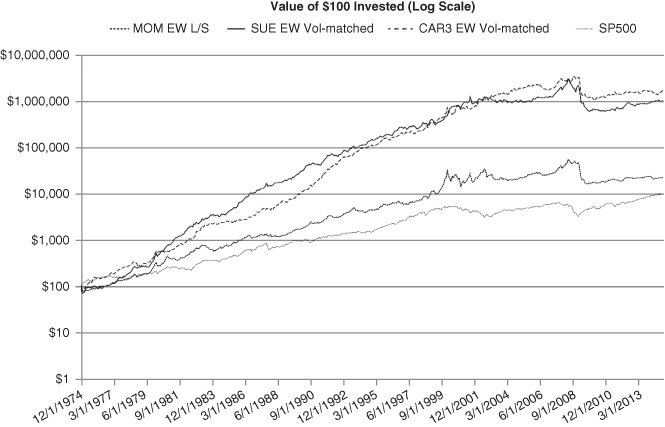
Figure A1.1 Fundamental Momentum Returns
Table 2 in the Novy-Marx paper shows the results of time-series regressions: Panel A shows that UMD loads heavily on both SUE and CAR3. A few key findings: First, after controlling for earnings momentum and various risk factors (e.g., market exposure, size exposure, and value exposure), price momentum no longer produces alpha. Panels B and C of Table 2 show that the alphas associated with SUE and CAR3 are highly significant. Novy-Marx concludes that earnings momentum “subsumes” price momentum, since it seems to explain the entire effect.
But the paper's assault on price momentum goes further. There are two additional findings in the paper:
- Excluding the price momentum factor from earnings momentum factors improves the earnings momentum performance, while excluding earnings momentum from price momentum worsens the price momentum performance. This is in the context of a long/short strategy run at a scaled volatility of 10 percent.
- Controlling for price momentum when constructing earnings momentum strategies can help reduce volatility and eliminate crashes to a large extent. (The price momentum strategy is known for being sensitive to market cycles5 and is more volatile in poor market environments.6)
In summary, Novy-Marx's findings highlight what has been known for a while in academic research, namely, that the anomalous returns associated with a price momentum strategy seem to be associated with an underreaction to earnings news. However, Novy-Marx points out that price momentum is not the right proxy to capture this underreaction effect, instead we should be focused on earnings momentum metrics and the underreaction to unexpected earnings surprises. According to Novy-Marx's analysis, price momentum doesn't matter—earnings momentum does. However, this evidence directly contradicts the analysis from Chan, Jegadeesh, and Lakonishok, who show that both earnings momentum and price momentum play a role in identifying anomalous returns.
Because the results of price momentum and earnings momentum are mixed, we did our own investigation of this research under our own research conditions. We focus on the universe of stocks we've used throughout this book: mid- and large-cap US traded common stocks. We create the portfolios described in Novy-Marx and examine the top and bottom decile portfolios created from our universe based on price momentum, SUE, and CAR3. Monthly rebalanced portfolios are formed by equal-weighting the firms and the returns run from January 1, 1975, through December 31, 2014. Returns are shown gross of any fees.
Table A1.1 shows the top decile (long portfolio) for the measures, while Table A1.2 shows the bottom decile (short portfolio) for the measures.
Table A1.1 Top Decile Portfolio Summary Statistics
| Price Momentum | SUE | CAR3 | SP500 | |
| CAGR | 19.81% | 19.64% | 16.79% | 12.31% |
| Standard Deviation | 25.73% | 18.85% | 22.28% | 15.10% |
| Downside Deviation | 18.21% | 14.28% | 15.40% | 10.95% |
| Sharpe Ratio | 0.65 | 0.80 | 0.60 | 0.53 |
| Sortino Ratio (MAR |
0.91 | 1.04 | 0.85 | 0.71 |
| Worst Drawdown | –58.59% | –56.08% | –59.05% | –50.21% |
Table A1.2 Bottom Decile Portfolio Summary Statistics
| Price Momentum | SUE | CAR3 | SP500 | |
| CAGR | 6.07% | 11.31% | 8.12% | 12.31% |
| Standard Deviation | 26.48% | 19.39% | 23.06% | 15.10% |
| Downside Deviation | 18.00% | 13.85% | 16.44% | 10.95% |
| Sharpe Ratio | 0.17 | 0.40 | 0.25 | 0.53 |
| Sortino Ratio (MAR |
0.24 | 0.55 | 0.34 | 0.71 |
| Worst Drawdown | –80.96% | –62.18% | –69.51% | –50.21% |
The price momentum and the SUE portfolio have the best top decile performance (long leg in a long/short strategy), while price momentum has the worst bottom performance (short leg in a long/short strategy). At first glance, one might assume that the best long/short portfolio would be associated with the price momentum strategy, since the spread between the long and the short portfolio is greatest. That assumption is wrong. We examine the performance of monthly rebalanced long/short portfolios that go long the top decile portfolio and short the bottom decile portfolio. The results are tabulated in Table A1.3.
Table A1.3 Long/Short Momentum Portfolio Annual Returns
| Price Momentum (L/S) | SUE (L/S) | CAR3 (L/S) | SP500 | |
| CAGR | 14.59% | 12.38% | 12.83% | 12.31% |
| Standard Deviation | 25.28% | 8.30% | 8.04% | 15.10% |
| Downside Deviation | 21.94% | 6.29% | 6.13% | 10.95% |
| Sharpe Ratio | 0.48 | 0.87 | 0.95 | 0.53 |
| Sortino Ratio (MAR |
0.55 | 1.13 | 1.22 | 0.71 |
| Worst Drawdown | –71.36% | –37.93% | –29.26% | –50.21% |
The results in Table A1.3 show that the price momentum long/short portfolio has the highest compound annual growth rate (CAGR); however, this strategy has the highest risk. On balance, the performance is relatively weak on a risk-adjusted basis. In contrast, the SUE and CAR long/short portfolios' Sharpe and Sortino ratios are almost double that for the price momentum long/short portfolio. To make matters worse, the drawdown for the price momentum long/short portfolio (71.36%) is close to double that of the SUE (37.93%) and CAR3 (29.26%) long/short portfolios. To summarize, the long/short SUE and CAR3 portfolios look better than the price momentum portfolio and this is the core evidence that Novy-Marx rests on to highlight that price momentum is inferior to—and subsumed by—earnings momentum.
Thus far, we have identified that long-only price momentum is a promising strategy, but long/short SUE and CAR3 are much better long/short concepts in terms of risk-adjusted returns. However, as we learned in Chapter 4, the stand-alone performance of a strategy, while relevant, does not always tell us the complete story. For example, in Chapter 4, we look at the performance of long/short price momentum in Japan, which is a market where momentum is arguably a poor performer on stand-alone basis. But this compartmentalized focus on momentum ignores the fact that combining long/short momentum with a long/short value approach actually allows an investor to create the most robust portfolio market neutral portfolio. Why? Because long/short value and momentum share an incredible attribute: they are strongly negatively correlated. This means that the two strategies tend to work well at different times. And this diversification benefit associated with momentum cannot be captured by a Sharpe ratio. Sounds great, but how can we quantify this benefit? We take a simple factor analysis approach to ascertain how the three various long/short momentum strategies load on common risk factors related to market risk, size risk, and value risk.7 The results are shown in Table A1.4.
Table A1.4 Long/Short Momentum Portfolio Factor Loadings
| Price Momentum (L/S) | SUE (L/S) | CAR3 (L/S) | |
| Alpha (annual) | 0.16 | 0.08 | 0.09 |
| p-value | 0.0001 | 0.0000 | 0.0000 |
| RM-RF | –0.28 | –0.03 | –0.10 |
| p-value | 0.0128 | 0.4421 | 0.0024 |
| SMB | 0.45 | –0.06 | 0.08 |
| p-value | 0.0377 | 0.2141 | 0.1644 |
| HML | –0.67 | –0.10 | –0.13 |
| p-value | 0.0013 | 0.1195 | 0.0160 |
The factor analysis shows that all three strategies have alpha—which has already been identified by previous research. However, we focus on the value factor (HML), which identifies the statistical relationship between a given strategy and a generic long/short value portfolio. The price momentum strategy has a highly significant loading of –0.67, making it a prime candidate for pairing with a value strategy. However, the earnings momentum strategies, SUE and CAR3, have value loadings that are closer to zero. The data suggest that these strategies may not be as useful, from a portfolio perspective, for pooling with a value-centric portfolio.
To get a better feel for the practical implications of the analysis above, we conduct an empirical test. Over the January 1, 1975, to December 31, 2014, sample period, we form four portfolios that allocate 50 percent to value and 50 percent to momentum every month. The value portfolio is represented by a portfolio that is long the top decile of firms ranked on EBIT/TEV (Earnings before Interest and Taxes/Total Enterprise Value) and rebalanced annually. The value portfolio is combined with the price momentum strategy, the SUE strategy, the CAR3 strategy, and the frog-in-the pan momentum portfolio (the four momentum-related strategies are all monthly rebalanced). In Chapters 5 through 8, we recommend a quarterly rebalanced portfolio, but here we use the monthly rebalanced portfolio to facilitate a fair comparison. Chapters 5 to 8 also show returns from 1974–2014, here we show returns from 1975–2014 due to data constraints on the SUE portfolios. All return streams are shown gross of any fees or transaction costs. Results are in Table A1.5.
Table A1.5 Value and Momentum Portfolio Annual Returns
| 50% Frog Momentum/ 50% Value | 50% Price Momentum/ 50% Value | 50% SUE/ 50% Value | 50% CAR/ 50% Value | |
| CAGR | 20.54% | 19.72% | 19.25% | 17.92% |
| Standard Deviation | 19.55% | 19.84% | 17.62% | 19.05% |
| Downside Deviation | 14.36% | 14.50% | 13.48% | 13.64% |
| Sharpe Ratio | 0.81 | 0.77 | 0.82 | 0.71 |
| Sortino Ratio (MAR |
1.10 | 1.04 | 1.06 | 0.98 |
| Worst Drawdown | –52.55% | –50.29% | –50.06% | –49.11% |
The combination portfolio of the frog-in-the-pan momentum portfolio and the value portfolio produce the highest CAGR and Sortino ratios. The SUE portfolio is also strong, with marginally weaker results. In short, while the results Novy-Marx presents on SUE are intriguing, and certainly worth consideration, when viewed through the practitioner lens, we believe this is a much ado about nothing situation. The results aren't powerful enough to suggest that price momentum is dead.8
IS THE 52-WEEK HIGH A BETTER MOMENTUM SIGNAL?
The 52-week high metric is widely reported and readily available to investors. But do investors respond rationally to this piece of information? Investors may react irrationally to 52-week high signals because of anchoring and framing biases. For example, irrational investors may take the 52-week high metric as a signal to sell without considering the fact that the current price may undervalue the security on a fundamental basis.
A paper written in 2012 by Malcom Baker, Xin Pan, and Jeffrey Wurgler9 examines the effect of reference points in mergers and acquisitions. The findings are quite astonishing—here is a summary taken from the abstract:
So the peak price (52-week high) actually influences the unconditional probability of merger completion—that certainly wasn't part of the efficient market hypothesis textbooks we were reading in graduate school! Clearly, the 52-week high affects merger and acquisition activity, but what about using the metric for stock selection? Intuitively, the 52-week high will be related to relative strength momentum measures that we've discussed throughout the book. But is it a better measure than traditional momentum calculations? In 2004, Thomas J. George and Chuan-Yang Hwang10 set out to write a paper to address this question.
George and Hwang's paper titled “The 52 Week High and Momentum Investing,” finds that the 52-week-high strategy is better than traditional momentum strategies. The conclusion of the paper is bold: “Returns associated with winners and losers identified by the 52-week high strategy are about twice as large as those associated with the other [momentum] strategies.”
The authors explain their result by suggesting that when good news has pushed a stock's price near a 52-week high, investors are reluctant to bid the price of the stock higher, even if the information warrants it. Essentially, the weird feeling of buying a stock when the chart is at a peak prevents stocks from reaching fundamentals. Fundamental information eventually is incorporated into the stock price and the price moves up, resulting in a “momentum-like” effect. Similarly, when bad news pushes a stock's price far from its 52-week high, traders are initially unwilling to sell the stock at prices that are perceived to be “too low.” However, fundamental news is eventually reflected in the stock price, prices drop, and anomalous returns are earned by shorting stocks near their 52-week lows.
What are we to make of these results? We spent the bulk of this book explaining that a momentum strategy should be built using only the past returns, while this paper claims that the profits can be doubled if one uses a 52-week-high indicator. To better understand the strategy we replicate the results from this paper and run them through our laboratory tests.
We first examine the results from the original paper. The paper compares three momentum strategies using a sample of all US traded stocks from 1963 to 2001:
- 1. Price momentum: The price momentum portfolio takes long (short) positions in the 30 percent top (bottom) performing stocks based on their past six months' returns and is rebalanced every six months.11
- 2. Industry momentum: In 1999, Toby Moskowitz and Mark Grinblatt12 develop an industry momentum screen. The universe of stocks is split into 20 industries, and a value-weight return is computed for each industry. The industry momentum portfolio takes long (short) position in stocks in the 30 percent top (bottom) performing industries.
- 3. 52-week-high momentum: The 52-week-high portfolio takes long (short) positions in stocks whose current price is close to (far from) the 52-week high. The distance from the 52-week high is measured by the price of the stock one month ago divided by the 52-week high in the previous year. So if we are standing on December 31, 2015, we divide the price on November 30, 2015, by the 52-week high November 30, 2014–2015.
For the three strategies listed above, the stocks within the long and short portfolios are equally weighted, held for six months, and reconstituted every month (to create overlapping portfolios). In Table 2 of the original paper, the authors find that the profits to the three long/short momentum strategies listed above are the highest (when excluding January) using the 52-week high screen. The paper also investigates which strategy is most effective, after controlling for various factors and market microstructure considerations. Regression results from Table 5 in the original paper show that 52-week high winner/loser dummy is a good predictor of future return—better than the past stock returns or industry factors.
The collective results suggest the 52-week high is a better trading signal than price momentum. But what do the results look like using our universe of stocks? It should be pointed out that the George and Hwang paper uses all stocks, and thus includes small-cap stocks, which can greatly skew results. In contrast, we stick to a mid- and large-cap universe that is relatively liquid and where the data are more robust. We form portfolios using the 52-week-high screening variable, and place stocks into deciles based on the ranking. Portfolios are reconstituted monthly, and are held for either one month, three months, or six months. For the portfolios with three- and six-month holding periods, overlapping portfolios are used. Portfolios are formed by equal-weighting the firms, and the returns run from January 1, 1974, through December 31, 2014. Returns are shown gross of any fees. For each decile, we plot the CAGR in Figure A1.2.

Figure A1.2 Decile Returns to 52-Week High Screen
The results in Figure A1.2 document a few important findings. First, we notice that for the three- and six-month holding periods, there is a near monotonic increase in the CAGR as one moves from decile 1 (furthest away from 52-week high) up to decile 10 (closest to the 52-week high). This should be expected as the paper goes long the top three deciles and shorts the bottom three deciles to form the 52-week-high L/S portfolio discussed in the paper. The paper also focuses their discussion around the portfolios that are held for six months, which, not surprisingly, have the best performance. However, for the monthly rebalanced version of the 52-week-high strategy, the results break down dramatically. In other words, they fail a simple robustness test. When results are fragile to reasonable changes in portfolio construction, we get queasy that data mining may explain the analysis.
To make matters worse for the 52-week-high strategy, a basic long strategy that buys the portfolio of stocks based on nearness to the 52-week high isn't that compelling. For example, the top decile 52-week-high portfolio, held for 3 months, earns a 14.15 percent CAGR. Not bad, relative to the market before transaction costs, but this CAGR is much lower than the simple price momentum top decile portfolio (discussed in Chapter 5) held for three months, which earned a 17.10 percent CAGR over the same period.
Overall, we are impressed with the story behind the 52-week-high concept, but we feel there is no robust evidence that the strategy is more effective than relative strength price momentum strategies. Nevertheless, the 52-week-high evidence does point in the general direction of the price momentum anomaly and serves as another data point, which highlights that momentum strategies likely exploit mispricing caused by marketwide underreaction to news.
CAN ABSOLUTE STRENGTH IMPROVE RELATIVE STRENGTH MOMENTUM?
“Absolute Strength: Exploring Momentum in Stock Returns,” by Huseyin Gulen and Relitsa Petkova,13 has an interesting twist on standard relative strength momentum strategies. As we've discussed throughout this book, the academic research community captures the generic momentum strategy by ranking firms on their past 12-month momentum (ignoring last month's return). Portfolios are then formed on these rankings. Most research papers long the winners and short the losers. However, the classification of a “winner” stock and a “loser” stock changes over time. During the Internet bubble, to be classified as a “winner” a firm needed to have a past momentum score of around 250 percent (near the peak). During the 2008 financial crisis, a “winner” stock would be any stock with a return above negative 5 percent. Clearly, relative strength winners can have wide-ranging returns (the same wide-ranging result is seen on relative strength losers).
The authors explore the idea that perhaps a momentum strategy can be improved by focusing on the “absolute” strength score. The idea is to look back each month at the historical cutoffs for winners and losers, while using all available returns to create the cutoffs. An example will illustrate the methodology more clearly. Imagine it is January 31, 1965, and we examine all the momentum scores (past 12-month momentum, skipping the most recent month) for all stocks measured in January, using every year available prior to 1965. This would be all the momentum scores on January 31, 1927, January 31, 1928 … , and January 31, 1965. From this sample set, identify the 10th and 90th percentile values and use these as the “absolute” momentum cutoffs. The cutoff analysis is completed each month, so the percentile values are dynamic over time.
The absolute momentum cutoffs ensure that the definition of a winning and a losing stock are more consistent over time. Using results from the paper, the “winning” stock cutoff is near 60 percent, while the “losing” stock cutoff is around negative 35 percent. Portfolios are formed using stocks that meet the cutoff points. And while this approach has intuitive appeal, the portfolio strategy will create stock portfolios with differing numbers of stock holdings. In some cases, the number of stock holdings can be extreme. For example, a figure from the original paper shows that during the 2008 financial crisis, the number of winners drops close to zero, while the number of losers goes above 1,500. A relative strength momentum rule on the other hand, will always buy the top 10 percent and sell the bottom 10 percent of the universe. So if there are 5,000 firms in the universe, the relative strength portfolio would buy 500 stocks and sell 500 stocks, keeping the portfolio size in balance.
Construction issues aside, how does this absolute momentum portfolio perform? The author's strategy that buys absolute strength winners and sells absolute strength losers delivers a risk-adjusted return of 2.42 percent per month from 1965 to 2014 and 1.55 percent per month from 2000 to 2014. The baseline results to the long/short portfolios are impressive.
We're a bit skeptical of the results based on the universe used by the authors. Their universe includes microcaps stocks, which make up around 60 percent of the names in the CRSP universe, but only about 3 percent of the market cap according to Fama and French 2008.14 Imagine trying to long or short hundreds of microcap stocks!
To assess the validity of the absolute momentum results we decided to perform the same analysis on a universe of mid- and large-cap US stocks. We reconstruct the absolute momentum signal every month according the cookbook outlined in the original paper. Figure A1.3 plots the breakpoints over time. The return breakpoints are similar to those in the paper: the “winning” stock cutoff is around 60 percent, while the “losing” stock cutoff is around –35 percent. We only include stocks in the winner portfolio if they are above the winner cutoff and only include stocks in the loser portfolio if they are below the loser cutoff. As mentioned previously, this approach introduces an odd portfolio construction element. Figure A1.4 highlights the number of firms in the high and low absolute momentum portfolios across time and compares these portfolio sizes to the standard price momentum approach that buys the top 10 percent relative strength stocks and shorts the bottom 10 percent relative strength stocks.
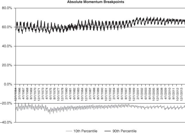
Figure A1.3 Absolute Momentum Breakpoints

Figure A1.4 Absolute Momentum Number of Firms
Similar to the original paper, there are extreme variations in portfolio sizes. During the financial crisis the absolute momentum portfolio is long one firm in January 2009, while the absolute momentum portfolio is short over 800 stocks.
We next assess the performance of the absolute momentum long/short strategy. We examine long/short returns to the equal-weighted monthly rebalanced portfolios from January 1965 to December 2014. All returns shown are total returns but are gross of any fees and transaction costs. The results are shown in Table A1.6.
Table A1.6 Absolute Momentum Long/Short Returns
| Absolute Strength (L/S) | Relative Strength (L/S) | SP500 | |
| CAGR | 25.28% | 17.97% | 10.01% |
| Standard Deviation | 23.26% | 24.02% | 15.04% |
| Downside Deviation | 17.57% | 20.58% | 10.64% |
| Sharpe Ratio | 0.88 | 0.61 | 0.38 |
| Sortino Ratio (MAR |
1.17 | 0.71 | 0.54 |
| Worst Drawdown | –68.27% | –70.86% | –50.21% |
The results are similar to the paper: the absolute momentum long/short portfolio outperforms the relative strength portfolio on a variety of metrics. To dig a bit deeper into the absolute momentum concept, we look at the performance of the long and short portfolios, separately.
Table A1.7 shows the results to the four portfolios (Absolute Strength Winners and Losers; Relative Strength Winners and Losers). Portfolios are equal-weighted and rebalanced monthly from January 1965 to December 2014. All returns shown are total returns but are gross of any fees and transaction costs.
Table A1.7 Absolute Momentum Long-Only Portfolio Returns
| Absolute Momentum Winner Portfolio | Relative Momentum Winner Portfolio | Absolute Momentum Loser Portfolio | Relative Momentum Loser Portfolio | |
| CAGR | 18.91% | 18.74% | –3.42% | 2.40% |
| Standard Deviation | 24.85% | 25.11% | 26.17% | 26.20% |
| Downside Deviation | 17.06% | 17.41% | 17.09% | 17.39% |
| Sharpe Ratio | 0.63 | 0.62 | –0.19 | 0.03 |
| Sortino Ratio (MAR |
0.91 | 0.89 | –0.29 | 0.04 |
| Worst Drawdown | –65.09% | –58.40% | –94.10% | –82.01% |
Examining the results, the long-only “winner” portfolios are similar and there is little marginal benefit of an absolute momentum strategy relative to a classic price momentum strategy. The absolute momentum loser portfolio, however, is much worse than the relative momentum loser portfolio. These results suggest that the short leg drives the performance difference between the long/short absolute momentum strategy and the long/short relative momentum strategy.
Another potential issue is that the absolute momentum rule can create portfolios with varying sizes from month to month. Alternatively, the relative strength signal creates a highly consistent N in the portfolio from month to month. Indirectly, the absolute momentum rule opens an investor up to a lot of risk that may not be captured in a backtest. For example, in January 2009, the absolute momentum portfolio is long a single stock and the absolute momentum portfolio is short over 800 stocks. We don't know many investors who would consider it prudent to hold a single stock portfolio. Obviously, this didn't have a huge effect historically, but out of sample this could create serious consequences.
CAN THE VOLATILITY OF MOMENTUM BE CONSTRAINED?
A negative aspect to momentum investing is the fact that a high-momentum portfolio tends to have large drawdowns and gut-wrenching volatility. On the one hand, this is a terrible characteristic, but on the other hand, this is why momentum is sustainable—it is not easy to “arbitrage.” But perhaps there is a better way to manage the volatility of momentum strategies. Yufeng Han, Guofu Zhou, and Yingzi Zhu make a good attempt in their paper, “Taming Momentum Crashes: A Simple Stop-Loss Strategy.” The authors apply a simple stop-loss rule to the classic long/short momentum portfolio.15 The results are impressive. Using a 10 percent stop-loss rule, the authors drop the maximum monthly loss from negative 49.79 percent to negative 11.36 percent and the Sharpe ratios are more than doubled.
The specifics of the trading strategy can be summarized in three rules:
- Rebalance the long and short book monthly by sorting stocks on their past returns (the paper uses the last seven months' returns, excluding the most recent month).
- Monitor the long portfolio daily: If a long position declines by X percent (e.g., 10), sell the position and invest it in the risk-free rate until the end of the month.
- Monitor the short portfolio daily: If a short position rises by X percent (e.g., 10), cover the position and invest any proceeds in the risk-free rate until the end of the month.
Table A1.8 shows the original figures from the paper.
Table A1.8 Equal-Weighted Stop-Loss Momentum Monthly Returns
| Variable | Avg Ret (%) | Minimum (%) |
| Panel A: Original Momentum | ||
| Market | 0.65 | –29.10 |
| Losers | 0.24 | –39.50 |
| Winners | 1.24 | –33.06 |
| WML | 0.99 | –49.79 |
| Panel B: Stop Loss at 10% | ||
| Losers | –0.42 | –39.27 |
| Winners | 1.27 | –12.87 |
| WML | 1.69 | –11.36 |
| Panel C: Stop Loss at 5% | ||
| Losers | –0.83 | –36.34 |
| Winners | 1.53 | –8.48 |
| WML | 2.35 | –8.94 |
Not only does the portfolio have smaller monthly drawdowns, but the average returns increase with the use of the stop-loss rules! If we examine the winners minus losers (WML) long/short portfolio the average monthly returns are highest using the 5 percent rule. Any strategy that can lower drawdowns and increase returns is pretty compelling and worth a second look.
Of course, nothing in financial markets is ever easy, although sometimes it looks that way. A downside of the stop-loss approach is that the strategy requires daily analysis of every stock position, which may be quite difficult—not to mention costly—for many investors to implement unless they use trailing stop loss orders. Also, from the perspective of a long-only investor, which is the focus of our book, the benefits to a stop-loss strategy are muted. For example, a momentum strategy with a 10 percent stop-loss rule has a 1.27 percent average monthly return, which is similar to a long-only buy and hold momentum strategy, which earns a 1.24 percent average monthly return. That said, there is a risk management benefit to a stop-loss approach, which we will examine in more detail.
Similar to our prior analysis, we examine the stop-loss strategy under our own research conditions. We examine a mid- to large-cap US traded universe and we focus our analysis on the long-only portfolios. All returns are gross, and no management fee or transaction costs are applied. We examine the returns from January 1, 1927, to December 31, 2013, to cover the same sample period analyzed in the paper. We examine the following four portfolios:
- 1. High momentum: Top 10 percent of firms ranked on their past momentum (total return over the past 12 months ignoring last month). Portfolio is monthly rebalanced and equal weighted.
- 2. High momentum with 10 percent stop-loss rule: Top 10 percent of firms ranked on their past momentum (total return over the past 12 months ignoring last month). Portfolio is monthly rebalanced and equal weighted. If during the month any individual stock position is down 10 percent, sell the security and remain in cash until the end of the month, at which time the portfolio is rebalanced into the top 10 percent of momentum firms.
- 3. High momentum with 5 percent stop-loss rule: Top 10 percent of firms ranked on their past momentum (total return over the past 12 months ignoring last month). Portfolio is monthly rebalanced and equal weighted. If during the month any individual stock position is down 5 percent, sell the security and remain in cash until the end of the month, at which time the portfolio is rebalanced into the top 10 percent of momentum firms.
- 4. SP500: Total return of the S&P 500 Index.
The results of the analysis are presented in Table A1.9.
Table A1.9 Momentum Stop-Loss Performance
| High Momentum | High Momentum 10% Stop-Loss | High Momentum 5% Stop-Loss | SP500 | |
| CAGR | 19.34% | 15.47% | 15.29% | 9.91% |
| Standard Deviation | 24.78% | 22.19% | 18.31% | 19.18% |
| Downside Deviation | 18.26% | 12.73% | 8.36% | 14.26% |
| Sharpe Ratio | 0.70 | 0.61 | 0.68 | 0.41 |
| Sortino Ratio (MAR |
0.87 | 0.93 | 1.31 | 0.44 |
| Worst Drawdown | –71.73% | –64.02% | –48.11% | –84.59% |
The long-only generic momentum portfolio generates a much higher CAGR than the risk-managed portfolios; however, the risk profile is arguably better for the stop-loss systems. However, the risk profile is highly dependent on the stop-loss rule examined, which hints toward a robustness issue. Relative to the 10 percent stop-loss rule, generic momentum is a better strategy, but relative to a 5 percent stop-loss rule, generic momentum is worse on a risk-adjusted basis.
On net, the stop-loss rule is interesting; however, risk management via stop-loss is not the only option. One can apply a simple long-term trend-following rule16 and/or a time-series momentum rule17 on a long-only momentum strategy and avoid the complexity and operational commitment required for a daily-assessed momentum portfolio. For example, consider a simple time-series momentum trading rule that is long the momentum portfolio if the past 12 month return on the S&P 500 is above the risk-free rate, otherwise, the portfolio is investing in risk-free bonds.
Here are the four portfolios we test:
- 1. High momentum w/TSMOM: Top 10 percent of firms ranked on their past momentum (total return over the past 12 months ignoring last month). Portfolio is monthly rebalanced and equal weighted. A 12-month time-series momentum-trading rule is applied each month.
- 2. High momentum: Top 10 percent of firms ranked on their past momentum (total return over the past 12 months, ignoring last month). Portfolio is monthly rebalanced and equal weighted.
- 3. High momentum with 10 percent stop-loss rule: Top 10 percent of firms ranked on their past momentum (total return over the past 12 months ignoring last month). Portfolio is monthly rebalanced and equal weighted. If during the month any individual stock position is down 10 percent, sell the security and remain in cash until the end of the month, at which time the portfolio is rebalanced into the top 10 percent of momentum firms.
- 4. High momentum with 5 percent stop-loss rule: Top 10 percent of firms ranked on their past momentum (total return over the past 12 months ignoring last month). Portfolio is monthly rebalanced and equal weighted. If during the month any individual stock position is down 5 percent, sell the security and remain in cash until the end of the month, at which time the portfolio is rebalanced into the top 5 percent of momentum firms.
The returns run from January 1, 1928, to December 31, 2013 (we don't include 1927 because we need to use 12 months of data to get the TSMOM rule). Results are gross of fees. All returns are total returns and include the reinvestment of distributions (e.g., dividends).
The results from Table A1.10 highlight that a simple monthly reviewed risk management rule applied at the portfolio level can achieve the same level of risk control, but with a lot less complication, than daily-assessed stop-loss rules.
Table A1.10 Time-Series Momentum Performance
| High Momentum TSMOM | High Momentum | High Momentum 10% Stop-Loss | High Momentum 5% Stop-Loss | |
| CAGR | 16.57% | 18.93% | 15.06% | 14.88% |
| Standard Deviation | 20.97% | 24.84% | 22.23% | 18.32% |
| Downside Deviation | 16.80% | 18.31% | 12.75% | 8.36% |
| Sharpe Ratio | 0.68 | 0.69 | 0.59 | 0.66 |
| Sortino Ratio (MAR |
0.75 | 0.85 | 0.91 | 1.26 |
| Worst Drawdown | –50.99% | –71.73% | –64.02% | –48.11% |
If investors are interested in managing the volatility of their portfolio, werecommend that investors first focus on achieving the best possible long-only momentum portfolio and combine it with the best possible long-only value portfolio. Once that is achieved, and the investor is capturing the highest expected equity premium on a risk-adjusted basis, the investor can deploy risk-management rules at the portfolio level. Although a detailed discussion of this approach is beyond the scope of this book, we recommend that investors focus on simple trend-following and time-series momentum type rules to facilitate portfolio-level risk management.