
CHAPTER 7
Momentum Investors Need to Know Their Seasons
“… planetary aspects and sunspot activity have significant power predicting anomalies' returns.”
—Robert Novy-Marx, Journal of Financial Economics1
Seasonality, broadly defined in the context of stock market research, refers to the idea of building timing signals based on the calendar. Turn on any financial news outlet and there typically is a discussion about seasonality. One of the more popular concepts is, “Sell in May and Go Away,” which suggests that investors go to cash before June and get back in to the market in November. However, a 2014 Novy-Marx paper titled “Predicting Anomaly Performance with Politics, the Weather, Global Warming, Sunspots, and the Stars,”2 highlights an important point: One needs to be skeptical of seasonality-type claims. Moreover, Cherry Zhang and Ben Jacobsen review over 300 years of UK stock market data and conclude that documented seasonality effects should be digested with a healthy dose of skepticism.3 That said, a recent paper by Matti Keloharju, Juhani Linnainmaa, and Peter Nyberg using the latest data and research techniques shows that stock market return seasonalities exist in almost every asset class, are remarkably persistent over time, and are extremely large.4 At a high level, seasonality makes sense: Institutional and behavioral incentives plausibly can drive supply and demand shocks that create robust seasonality effects. We consider the effects of window dressing and tax incentives in this chapter.
But why are we even talking about seasonality and how is this related to momentum investing? Let us explain. Five years ago, we started working on what we considered a “unique” idea that related seasonality to momentum investing. Our hypothesis was that window dressing and tax-loss selling could be exploited to maximize the benefits of a traditional seasonality-agnostic momentum strategy. We conducted a battery of empirical tests and summarized all our data. The results were stunning. What was even more exciting was that fact that our idea had never been published in what is considered a top-tier academic finance journal, a descriptor that is typically reserved for The Journal of Finance, Journal of Financial Economics, and the Review of Financial Studies. Of course, as a last-minute check, we reviewed what academic researchers consider to be the “nonserious research” journals, also referred to as the practitioner journals (e.g., Financial Analyst Journal or The Journal of Portfolio Management). Turns out, it was good we reviewed these journals. Richard Sias had already published our results in a Financial Analyst Journal issue in 2007.5 Our initial reaction was disappointment, because as academic researchers we had hoped we could publish a new idea, but at the same time we were happy because our independent analysis of seasonality in the context of momentum was confirmed—and already discovered—by an independent party. So to make a long story short, Sias got to the front of the line before we could get there. We like his idea, obviously, but to really understand the results from Sias's paper, we need to dig into some marketplace incentives. We first analyze the motivations behind window dressing and tax-loss selling and then explore why they are important for momentum investing in the sections that follow.
WINDOW DRESSING
In the retail business, window dressing refers to the practice of arranging merchandise in a store window to make it appear as attractive as possible. Window dressing works because it brings customers into the store, even if the merchandise is not as good as it looks in the window. In the financial services industry, fund managers leverage the same concept.
The concept of window dressing goes back—literally—to the beginning of formal economic research. Window dressing in economics, for readers unfamiliar with the term, is a behavior exhibited by finance professionals to mislead and cater to the whims of less sophisticated clients. The American Economic Review, which is considered one of the oldest and most respected scholarly journals in economics, was established in 1911. And in its initial publication, Edwin Kemmerer,6 an established economics professor and advisor to foreign governments, mentions the term window dressing to describe the New York money market near the end of the year.
Here is how window dressing works in practice: Fund managers know they must report their holdings on quarterly statements, which will get mailed to their clients. But the last thing poor-performing managers want their clients to see is their loser stocks that underperformed the market. In other words, they don't want investors seeing loser stocks in their “window,” which people will be viewing. To manage around this scenario, just before the statement reporting date the manager will sell their loser stocks and buy all the recent winning stocks so they look good on the statement, which is analogous to a “window” for a bricks and mortar retailer. Voila! The window now looks much more enticing.
Obviously, window dressing is not going to be a cure for bad performance and this tactic is not going to trick sophisticated clients, but the fund manager's hope is that window dressing activity will at least make them appear to have been doing something smart, and reduce client questions when they receive their statements. For example, consider the two scenarios between a client and a fund manager in 2002, following the bursting of the Internet Bubble:
- Scenario 1: “Geez, you underperformed by 10 percent. And wow, you owned Pets.com, which is down a lot? … Why do you own that horrible stock? You really must be an idiot!”
- Scenario 2: “Geez, you underperformed by 10 percent. But it looks like you own Berkshire Hathaway—that is a stable value stock that has done well. You probably had an unlucky stretch, but you seem like a good manager.”
Clearly, the manager would much rather face the reaction in scenario 2 as opposed to the one in scenario 1.
Of course, this scenario sounds like a great story, but what is the evidence that sneaky mutual fund managers actually engage in window dressing? Some authors think window dressing represents an anecdotal story, but not reality. For example, Gang Hu, David McLean, Jeff Pontiff, and Qinghai Wang find little evidence of window dressing by institutional investors.7 Others disagree. Consider Marcin Kacperczyk, Clemens Sialm, and Lu Zheng's paper “Unobserved Actions of Mutual Fund Managers.”8 They create a tool for addressing the window dressing hypothesis by creating a return gap measure. The return gap measure examines the difference between the realized returns to the mutual fund and the returns to the buy-and-hold portfolio that is most recently disclosed on the quarterly statement. The goal of the return gap measure is to identify, as is aptly put in the title, the unobserved actions of the mutual fund manager. The data suggests that some unobserved actions may create value (e.g., manager stock-picking skill), while other unobserved actions may destroy value (e.g., window dressing tactics). And the creation and destruction of value appears to be persistent across time for each fund. Unfortunately, the return gap is a relatively crude measure, and because there are too many variables to control for in the environment, a better experiment is needed to pinpoint window dressing.
David Solomon, Eugene Soltes, and Denis Sosyura9 identify a better laboratory to examine window dressing effects. Specifically, they examine how the media spotlight affects fund flows and window dressing. Their main finding is the following: “Investors reward funds that hold stocks with high past returns, but only if these stocks recently received media coverage.” So funds holding stocks with high-visibility winners attract more capital flows than similar funds holding less visible winners. Any mutual fund manager armed with this information has economic incentives to window dress—the data shows it leads to more assets under management!
Window-dressing is a perplexing practice, and one would hope that it is not that widespread. However, a 2004 study by Jia He, Lilian Ng, and Qinghai Wang examines window-dressing behavior across a variety of institutions.10 Their findings support the window-dressing hypothesis—institutions that act as external money managers (e.g., banks, life insurance companies, mutual funds, and investment advisers) are more likely to window dress their portfolios compared to institutions that act as internal money managers (e.g., pension funds, colleges, universities, and endowments). Not to beat a dead horse, but a more recent 2014 paper by Vikas Agarwal, Gerald Gay, and Leng Ling11 finds the following: “Window dressing is associated with managers who are less skilled and who perform poorly … we find that window dressing is value-destroying and is associated, on average, with lower future performance.”
The collective evidence and incentives of fund managers suggest that window dressing is likely part of the mutual fund landscape. Studies show that this window dressing may lead to increased assets under management, which explains why mutual fund managers partake in the activity. We'll explore why this window-dressing may matter for momentum investing, but first we turn our attention to the research on tax-motivated trading.
TAX-MOTIVATED TRADING
Sidney B. Wachtel published a paper in 1942 discussing how tax considerations can lead to seasonality in stock returns from December to January.12 Michael S. Rozeff and William R. Kinney, Jr., published a more comprehensive empirical investigation of Wachtel's initial ideas in 1976.13 Rozeff and Kinney examined stock returns from 1904 to 1974. Their main finding is one that stands to this day—the “January” effect, or “turn of the year” effect in stock markets. The turn of the year effect is the empirical observation that stock prices increase during the month of January, and this increase is statistically higher than the other months of the year. The core hypothesis for the effect is related to tax incentives at year-end. End-of-year tax-loss selling pressure is intuitive—one might expect to see a negative supply shock from taxable individuals looking to book losses at the end of the year, which is reversed in the new year. Although the “tax hypothesis” is intuitively appealing, research following Wachtel and Rozeff and Kinney argues that the effect is complex and has all but disappeared since the early 1990s.14
Early skeptics of tax-induced seasonality include Richard Roll,15 Don Keim,16 and Marc Reinganum,17 all of whom published papers in 1983. Their work collectively found that the larger January returns are mainly found in smaller firms and, therefore, may not be as pervasive as previously thought. More recent studies, however, both published in 2004, leverage smarter empirical techniques to tease out a robust relationship between taxes and the turn of the year effect. These works include a paper by Honghui Chen and Vijay Singal18 and another by Mark Grinblatt and Tobias J. Moskowitz.19
But which investors drive tax-loss selling? Jay Ritter dug a bit further into this question and examined the buying and selling of individual investors near the turn of the year.20 By measuring the ratio of buys and sells of individual investors, he found that individual investors sell more near the end of the year, and buy more in the beginning of the year—so a seasonal pattern exists for individual investors, who tend to hold smaller stocks. James Poterba and Scott Weisbenner21 also found that tax-loss selling is driven by individual investors, not institutions. This finding makes sense, as many institutional investors do not pay taxes, and therefore make buying and selling decisions without worrying about tax consequences (wouldn't that be nice!). Similarly, in 1997, Richard Sias and Laura Starks22 examined turn-of-the-year returns of stocks. They found that returns of stocks with a higher level of individual interest underperform in late December and outperform in early January relative to stocks with higher levels of institutional interest. So it appears tax-loss selling (by individuals as opposed to institutions) is behind the seasonality of returns for certain stocks.
But not all research finds that tax-loss selling causes the turn-of-the-year effect. For example, in 1983, Philip Brown, Donald Keim, Allan Kleidon, and Terry Marsh23 examined the returns in the Australian equity markets. At the time, Australia had similar tax laws to the United States, but a June–July tax year. They found that Australian equity returns had a predicted effect on July returns, but they also found the same January effect documented in US markets. The authors' findings muddy the waters on the causal relationship between tax-loss selling and the turn of the year effect and suggest that there may be something else going on that explains the turn of the year effect. On net, the research suggests that there is likely some connection between tax incentives and seasonal stock returns at year-end, but researchers still don't fully understand the exact relationship.
GREAT THEORIES: BUT WHY DO WE CARE?
The window dressing and tax-related seasonality effects previously outlined are interesting academic exercises. We now try to understand how these incentives may drive seasonal effects that can improve momentum strategies. As discussed previously, institutional investors have window dressing incentives to buy winners before the quarter ends and sell losers. This behavior leads us to our first hypothesis:
- Hypothesis #1: Momentum profits are highest in quarter-ending months, as window-dressing may cause institutional demand flows into high momentum stocks and out of low momentum stocks.
Another hypothesis related to seasonality and momentum is that taxable investors will want to sell losers and let winners ride at year-end to minimize tax burdens. This leads us to our second hypothesis:
- Hypothesis #2: Tax incentives lead to strong momentum profits in December as winners are unlikely to experience selling pressure and losers are likely to suffer from selling pressure. However, these tax-related flows will be reversed at the beginning of the year.
If we combine both the window-dressing and tax-minimization hypotheses, we should see strong momentum profits in the months prior to a quarter end (March, June, September, and December) and an especially profitable month prior to year-end (i.e., December). We should also see poor momentum profits in January, when the tax incentives from the months prior retreat and the demand for losing and winning stocks reverts to normal levels (e.g., losing stocks get a positive demand shock and winning stocks get a negative demand shock).
Richard Sias tests all of the concepts outlined above. He finds strong evidence to support the notion that momentum is a highly seasonal anomaly.24 To assess momentum profits, Sias forms long/short portfolios that are long the top decile of stocks with the strongest past six-month holding period and short the decile of stocks with the weakest past six-month holding periods. Figure 7.1 showcases his long/short portfolio results.
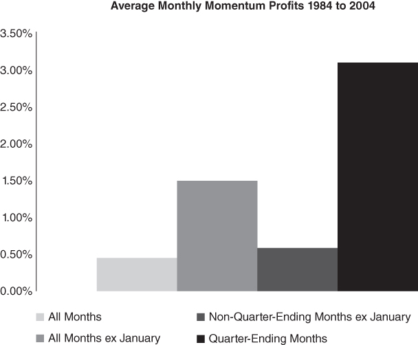
Figure 7.1 Momentum Seasonality from 1984 to 2004
Across all months, the average monthly profit from 1984 to 2004 is 0.45 percent per month, or roughly 5.4 percent a year. If one excludes January (“ex January,” in Figure 7.1), the portfolio earns 1.50 percent a month, or approximately 18 percent a year. January clearly matters, but so do quarter ending months. Momentum profits for quarter ending months average 3.10 percent a month, whereas non-quarter-ending months (excluding January) are 0.59 percent a month—a five-fold difference! And the pattern was stronger for stocks with high levels of institutional trading (where window-dressing incentives are highest) and was particularly strong in December (where tax incentives are strongest). The evidence is illuminating: Anyone devising a momentum strategy should incorporate aspects of seasonality into their algorithm. The results to long/short momentum portfolios in Figure 7.1 are in line with the window dressing and tax minimization hypotheses—near the end of a quarter, managers window dress their portfolios, so winning stocks do well (because they are being bought) while losing stocks do poorly (because they are being sold), and December has the strongest momentum returns across all months with an average monthly profit of 5.52 percent (reflecting both window dressing and tax pressures).
The evidence suggests that seasonality plays an important role in momentum-based stock selection strategies. We will leave the final comments on the subject to Sias, who says it best: “Investors attempting to exploit return momentum should focus their efforts on quarter-ending months …” In the next section we take Sias's advice and examine how to leverage seasonality to build a better stock selection momentum system.
MOMENTUM SEASONALITY: THE RESULTS
We start this section with a replication and extension of the results originally found in the Sias 2007 paper. We examine all mid- and large-capitalization stocks from January 1927 to December 2014. We examine the value-weight returns to quarterly rebalanced momentum portfolios using similar techniques from Chapters 5 and 6. The average monthly returns to the high momentum and low momentum (decile) portfolios are tabulated in Table 7.1.
Table 7.1 Average Returns by Month
| Low Momentum | High Momentum | Spread (High – Low) |
|
| January | 2.91% | 1.19% | –1.72% |
| February | –0.24% | 1.65% | 1.89% |
| March | 0.13% | 1.86% | 1.73% |
| April | 1.33% | 1.85% | 0.53% |
| May | 0.09% | 0.82% | 0.73% |
| June | 0.01% | 1.56% | 1.55% |
| July | 1.77% | 1.21% | –0.56% |
| August | 1.96% | 1.34% | –0.62% |
| September | –1.63% | –0.20% | 1.44% |
| October | –0.54% | 0.75% | 1.28% |
| November | 0.67% | 2.39% | 1.71% |
| December | 0.19% | 2.95% | 2.76% |
The takeaways from our analysis are similar to the original Sias paper. Examining the “Spread” column, January is a large “negative” month for momentum as low momentum outperforms high momentum. Quarter-ending months generally have the highest returns when comparing the low and high momentum portfolios. March has a positive momentum profit, but the outperformance compared to other months in the same quarter, are muted relative to June, September, and December. But as Sias points out in his original paper, the March result supports the window dressing hypothesis because institutions have a low incentive to window dress until later in the calendar year.
We can more easily visualize the spread between the high momentum average monthly returns and the low momentum average monthly returns in Figure 7.2. The results are quantitatively and directly similar to those found by Sias.

Figure 7.2 Momentum Spread from 1974 to 2014
Our replication and extended analysis of the Sias results give us confidence in the robustness of the original results (we conduct our tests on international data and come to similar conclusions). Now we need to identify how we can take this knowledge and leverage it for a momentum strategy. On one hand, we know that January is a large “negative” month for momentum and should be avoided, but do we really want to sell all our high momentum stocks at the end of December, buy all the low momentum stocks before January, and then rebalance back into high momentum before February? In theory, this activity would make sense, but in practice this activity would likely be difficult due to market liquidity and frictional costs.
Our own analysis of frictional costs and market liquidity suggest that exploiting the December to January momentum effects are unrealistic for a reasonably sized portfolio, so we'll punt on this idea, but we can still exploit momentum seasonality. We can build our system to take advantage of quarter-ending window dressing as well as tax-induced incentives at year-end. But how do we exploit this knowledge? Because momentum profits are largest in quarter-ending months, and this is likely driven by managers who are window dressing their portfolio, we hypothesize that rebalancing before these quarter-ending months will yield the highest returns.
We test our hypothesis that smart rebalancing that exploits seasonality effects can improve a momentum strategy. Recall from Chapters 5 and 6 that we examine the results to momentum portfolios using overlapping portfolios with a three-month holding period. To remind the reader, overlapping portfolios work as follows: We are standing at the end of the month on December 31, 2014. We calculate a generic momentum metric and use one-third of our capital to buy high-momentum stocks. These stocks stay in the portfolio until March 31, 2015. On January 31, 2015, a month later, we use another one-third of our capital to buy high-momentum stocks based on momentum rankings on January 31, 2015. These stocks stay in the portfolio until April 30, 2015. On February 28, 2015, a month later, we use another one-third of our capital to buy high momentum stocks. These stocks stay in the portfolio until May 31, 2015. This process repeats every month and creates the overlapping portfolio effect. And the returns to the overlapping portfolios reflect a blend of the underlying portfolios being managed with the overlapping portfolio, which minimizes seasonal effects.
Of course, in a test for seasonality and momentum, creating overlapping portfolios—which are formed to minimize seasonal effects—is not the correct approach. If we are deliberately trying to take advantage of seasonal effects, we can examine quarterly nonoverlapping portfolios formed before quarter-ending months. This portfolio formation is more intuitive to many outside of academic research and has the ability to exploit quarterly momentum effects. Specifically, we assume we trade the nonoverlapping seasonal momentum portfolio at the end of February, May, August, and November to exploit the known momentum profits associated with March, June, September, and December. We hold this nonoverlapping portfolio for three months, which means there are four rebalances per year. We compare the performance of this portfolio against other nonoverlapping portfolios that do not rebalance before quarter end months. Our hypothesis is that the nonoverlapping quarterly rebalanced portfolio that exploits momentum seasonality benefits will perform better than the other portfolio constructs that are seasonality agnostic.
Like prior tests, we only examine mid- and large-capitalization stocks and portfolios are formed by value-weighting the firms. The analysis is from March 1, 1927, through December 31, 2014.25 We follow the process from Chapter 5, which is to (1) sort stocks based on their cumulative 12-month past returns (ignoring the most recent month) and (2) examine the top decile based on their past returns.
In Table 7.2, we examine the results to the strategy outlined above, by varying the rebalance period, using these four portfolios:
Table 7.2 Seasonality of Momentum Portfolio Annual Results
| Smart Rebalance | Average Rebalance | Dumb Rebalance | Agnostic Rebalance | |
| CAGR | 15.97% | 15.65% | 15.06% | 15.49% |
| Standard Deviation | 23.99% | 23.96% | 23.90% | 23.62% |
| Downside Deviation | 17.93% | 17.56% | 17.70% | 17.43% |
| Sharpe Ratio | 0.60 | 0.59 | 0.57 | 0.59 |
| Sortino Ratio (MAR |
0.72 | 0.71 | 0.68 | 0.71 |
| Worst Drawdown | –74.19% | –73.35% | –77.43% | –73.90% |
| Worst Month Return | –30.09% | –31.01% | –30.45% | –30.00% |
| Best Month Return | 32.35% | 39.53% | 31.15% | 33.88% |
| Profitable Months | 62.71% | 62.14% | 62.14% | 61.86% |
- Smart Rebalance: The smartest seasonality rebalanced portfolio. This portfolio is rebalanced on the close of trading in February, May, August, and November.
- Average Rebalance: This portfolio is rebalanced on the close of trading in January, April, July, and October.
- Dumb Rebalance: The least seasonality smart portfolio. This portfolio is rebalanced on the close of trading in December, March, June, and September.
- Agnostic Rebalance: The seasonality agnostic portfolio. This portfolio is an overlapping portfolio rebalanced every month and held for three months.
All the portfolio returns shown above are value-weighted. Table 7.2 shows the results.
The results in Table 7.2 confirm our hypothesis that momentum seasonality can be exploited via smarter rebalancing, at the margin. If we look at equal-weight portfolio results (not shown) the effects are magnified. The smart rebalance portfolio exploits both window dressing and tax incentive effects that drive momentum profits and thus performs the best among all the portfolio constructs. The worst-performing portfolio is the portfolio that systematically rebalances at the worst time from a momentum seasonality perspective. Finally, the agnostic rebalanced portfolio and the average rebalance portfolio have results that are in the middle between the smart and dumb rebalanced portfolios. The lesson learned is simple: Focus on seasonality when building momentum systems.
SUMMARY
In this chapter, we explore two institutional behaviors that potentially drive seasonality effects in the stock market: window dressing and tax minimization. Next, we highlight research that maps these two incentives to the profitability of momentum. Finally, we conduct our own analysis of seasonality and momentum profits. We end with an analysis of different rebalancing techniques and how they affect the profitability of generic momentum strategies. Our key takeaway is that an investor can exploit the seasonality of momentum profits by developing a rebalance program that is designed to maximize performance.