CHAPTER 5
Measuring the Benefits of Environmental Protection
5.0 Introduction
The efficiency framework discussed in the previous chapter appears to give us a very precise answer to the question: Are we polluting too much? Yes, if the marginal benefits of reduced pollution (both today and in the future) exceed the marginal costs of reduction. However, determining the efficient pollution level requires that we first devise accurate measures of both the benefits and costs of decreased pollution.
The benefits of pollution control can be divided into two categories: market benefits and nonmarket benefits. For example, cleaning up a river may lead to increases in commercial fish harvests, greater use of tourist services, and fewer medical expenses and days lost at work due to waterborne diseases. Measuring these market benefits in dollar terms is a natural approach.
However, economists have also devised methods for measuring nonmarket benefits. In our example, these would include increased recreational use of the river (boating, swimming and fishing), the enjoyment of greater species diversity in the river, and a reduction in premature death due to diseases contracted from contaminated water. Nonmarket benefits are measured by inferring how much money people would be willing to pay (or accept) for these benefits if a market for them did exist.
Complicating the measurement of nonmarket benefits is the need to estimate the risk associated with industrial pollutants. For example, consider the case of polychlorinated biphenyls (PCBs), industrial chemicals widely used until the late 1970s as lubricants, fluids in electric transformers, paints, inks, and paper coatings. PCB-contaminated waste dumps remain fairly widespread throughout the country today. PCB exposure is related to developmental abnormalities in people and causes cancer in laboratory animals. However, the risk to humans from exposure to low levels of PCBs is not precisely known and can only be determined to lie within a probable range. The need to estimate, rather than directly measure, both nonmarket benefits and risk means that benefit measures for pollution reduction are necessarily fairly rough.
By a similar token, the direct costs of reducing pollution can be measured in terms of the increased expense associated with new pollution-control measures and additional regulatory personnel required to ensure compliance. However, indirect costs resulting from impacts on productivity and employment can only be inferred.
The next two chapters will take a close look at the methods of measuring and comparing the benefits and costs of environmental cleanup. The principal conclusion is that benefit–cost analysis is far from a precise science. As a result, the “efficient” pollution level can be pinpointed only within broad boundaries, if at all.
5.1 Use, Option, and Existence Value: Types of Nonmarket Benefits
The nonmarket benefits of environmental protection fall into three categories: use, option, and existence values. Use value is just that value in use. Returning to our river example, if people use a clean river more effectively for swimming, boating, drinking, or washing without paying for the services, then these are nonmarket use values.
An environmental resource will have option value if the future benefits it might yield are uncertain and depletion of the resource is effectively irreversible. In this case, one would be willing to pay something merely to preserve the option that the resource might prove valuable in the future. In certain cases, option value may actually be negative; that is, people may value a resource today less than its expected future use value. However, in many important environmental applications, option value will be positive.1
Finally, economists have indirectly included moral concerns about environmental degradation, including empathy for other species, in their utilitarian framework under the heading existence value. For example, if a person believed that all creatures had a “right” to prosper on the planet, then he or she would obtain satisfaction from the protection of endangered species, such as the spotted owl or the right whale, even if these species had no use or option value. The desire to leave an unspoiled planet to one’s descendants (a bequest motive) also endows species or ecosystems with an existence value.
As an example of the potential importance of existence value, a survey-based study estimated that Wisconsin taxpayers were willing to pay $12 million annually to preserve the striped shiner, an endangered species of tiny minnow with virtually no use or option value. As we will see, the results of this type of study must be interpreted with care. However, these results do seem to indicate a substantial demand for the preservation of species for the sake of pure existence.2
The total value of an environmental resource is the sum of these three components:
5.2 Consumer Surplus, WTP, and WTA: Measuring Benefits
Having defined the types of benefits that nonmarket goods generate, the next step is measurement. The benefit measure for pollution reduction that economists employ is the increase in consumer surplus due to such a reduction. Consumer surplus is the difference between what one is willing to pay and what one actually has to pay for a service or product. A simple illustration: Suppose that it is a very hot day and you are thirsty. You walk into the nearest store perfectly willing to plunk down $1.50 for a small soft drink. However, you are pleasantly surprised to discover that the price is only $0.50. Your consumer surplus in this case is $1.00.
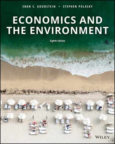
To illustrate how one would apply the consumer surplus concept to an environmental good, let us return to the example we employed in Chapter 3, in which Mr. Peabody has a private demand for the preservation of a trout stream in Appalachia. This demand may be based on his expected use, option, or existence value, or a combination of all three. His demand curve is illustrated in Figure 5.1.
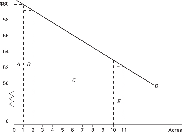
FIGURE 5.1 Consumer Surplus from Preservation
Initially, 10 acres of stream have been preserved. Assume that Mr. Peabody did not pay for this public good. Nevertheless, he still benefits from it. His consumer surplus from the first acre preserved is his willingness to pay (WTP) ($60), less the price ($0), or $60. We can graphically represent this consumer surplus area , lying below the demand curve and above the price (zero) for the first unit. Similarly, for the second acre, he is willing to pay about $59, which is also his consumer surplus as the good has a zero price. Consumer surplus from this unit is graphically represented as area . Peabody’s total consumer surplus from the initial 10 acres is graphically represented by the entire area .
Now suppose that a nature preservation society buys an extra acre of stream land. The benefits of this action for Peabody will be his increase in consumer surplus, area . But, this is just the price he is willing to pay for a 1-acre increase! For small increases in the stock of a public good enjoyed at no charge by consumers—such as trout streams or clean air or water—the price that people are willing to pay is a close approximation to the increase in consumer surplus that they enjoy.
This analysis suggests that one can measure the benefits of environmental improvement simply by determining people’s willingness to pay (WTP) for such improvement and adding up the results. However, WTP is not the only way to measure consumer surplus. An alternate approach would be to ask an individual his or her minimum willingness to accept (WTA) compensation in exchange for a degradation in environmental quality. In our example, Peabody could be persuaded to give up the 11th acre of stream in exchange for a little more than $52.3
In theory, WTP and WTA measures are both good approximations to the change in consumer surplus from a small change in a public good such as environmental quality. Economists predict that WTA will be a bit higher than consumer surplus, because individuals are actually made a bit richer when they are compensated for damage. On the other hand, WTP should be a bit lower than consumer surplus, as people will be made poorer if they actually have to pay for environmental improvement. However, the differences should not, in theory, be large as the income changes involved are not large.
Interestingly, however, the evidence does not support this prediction. What kind of evidence? Over the last few decades, economists have conducted many experiments in which the subjects were asked what they would pay for a wide array of both market and nonmarket items—a coffee mug, a hunting license, or improved visibility in the Grand Canyon, for example. A different pool of subjects would then be asked what they would be willing to accept in compensation to give up the mug, the license, or a haze-free day on the canyon rim. Even for everyday items such as coffee mugs, WTA values are typically higher than WTP values. And for nonmarket goods, such as preserving land from development, WTA values are typically seven times as high as WTP values.4
How can we explain the divergence between WTP and WTA benefit measures? One possibility is that, for psychological reasons, people are more willing to sacrifice to maintain the existing quality of the environment than they are to improve environmental quality beyond what is already experienced. People may adopt the status quo as their reference point and demand higher compensation to allow environmental degradation than they are willing to pay for making improvements. If this hypothesis, known as prospect theory, is correct, it would reshape our marginal benefit curve for pollution reduction as illustrated in Figure 5.2. Here, the marginal benefits of reduction dramatically rise just within the current levels of pollution.5
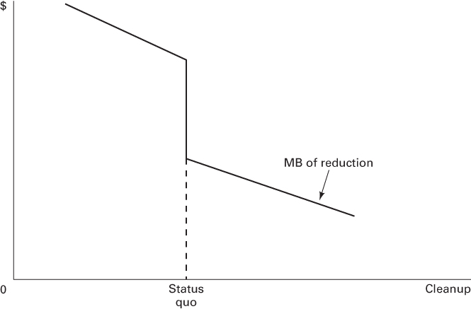
FIGURE 5.2 Prospect Theory and Marginal Benefits of Cleanup
A second explanation for the divergence between WTP and WTA is based on the degree of substitutability between environmental quality and other consumption goods. Consider, for example, a case in which people are asked for their WTP and WTA to reduce the risk of cancer death among members of a community from air pollution. A substantial reduction in the risk of death is something that, for many people, has few good substitutes. Nevertheless, a person whose income is limited will be able to pay only a certain amount for such a guarantee. On the other hand, because good substitutes for a reduced risk of death cannot be purchased, the compensation necessary for accepting such a risk might well be very large, even greater than the individual’s entire income.
Some have argued that this “no good substitutes” argument is of limited value in explaining the measured discrepancy between WTP and WTA. Can it really be true, for example, that a stand of trees in a local park has no adequate substitute for people in the community? Appendix 5A and Chapter 11 both take up in more detail the degree to which environmental goods and more common consumption items might actually substitute for one another in the provision of utility.
Regardless of the explanation, the WTA–WTP disparity is clearly important as economists try to place a value on improved or degraded environmental quality. The standard practice in survey research is to use WTP, on the basis that WTA measures are too difficult to estimate reliably. But, the right measure to use probably depends on the underlying property rights. If we think of common property resources such as clean air and water as belonging to “the people,” then WTA compensation for their degradation would appear to be the more correct measure of pollution damages. Both hazardous waste and oil spill legislation explicitly vest the public with rights to a clean environment by giving them the right to compensation for damages. Under this kind of property rights regime, WTP is clearly the wrong measure and will generate underestimates of the underlying resource value.6
Using either WTP or WTA as benefit measure generates one additional concern. Rich people, by the simple virtue of their higher incomes, will be willing to pay more for environmental improvement and will require more to accept environmental degradation. In other words, using WTP or WTA to assess the benefits of identical pollution-control steps in rich and poor areas will lead to a higher benefit value for the wealthy community. As we will see later, the ethical dilemma posed by this measurement approach appears to be strongest when comparing WTP and WTA for reduction in the risk of death or illnesses, between rich and poor countries.
5.3 Risk: Assessment and Perception
The first step in actually measuring the benefits of pollution reduction is to assess the risks associated with the pollution. As noted in the introduction, this can be a difficult process. Information on health risks comes from two sources: epidemiological and animal studies. Epidemiological studies attempt to evaluate risk by examining past cases of human exposure to the pollutant in question. For example, in the case of PCBs, developmental abnormalities such as lower birth weights, smaller head circumference, and less-developed cognitive and motor skills have been found in three separate communities of children whose mothers suffered substantial exposure. There is also limited evidence of a link between occupational exposure to PCBs and several types of cancer.
In animal studies, rats and mice are subjected to relatively high levels of exposure of the pollutants and examined for carcinogenic effect. PCBs have been found to generate cancers in animal studies. Translating this information to a human population requires two steps: first, the cancer incidence from high levels of exposure among animals must be used to predict the incidence from low levels, and, second, the cancer rate among animals must be used to predict the rate among people.
The assumptions made in moving from high-dose animal studies to low-dose human exposure constitute a dose–response model. A typical model might assume a linear relationship between exposure and the number of tumors, use a surface-area scaling factor to move from the test species to humans, and assume constant exposure for 70 years. Such a model would generate a much higher estimated risk of cancer for humans than if a different model were used: for example, if a safe threshold exposure to PCBs were assumed, if a scaling factor based on body weight were employed, or if exposure were assumed to be intermittent and short-lived.
The point here is that risk assessments, even those based on large numbers of animal studies, are far from precise. Because of this imprecision, researchers often adopt a conservative modeling stance, meaning that every assumption made in the modeling process is likely to overstate the true risk. If all the model assumptions are conservative ones, then the final estimate represents the upper limit of the true risk of exposure to the individual pollutant. Even here, however, the health risk may be understated due to synergy effects. Certain pollutants are thought to cause more damage when exposed to multiple toxic substances.
The combined epidemiological and animal evidence has led the U.S. Environmental Protection Agency (EPA) to label PCBs as probable human carcinogens. Due to concern about PCB (and other industrial pollutant) contamination of the Great Lakes, researchers undertook an evaluation of the risk of eating the Lake Michigan sport fish.7
Bearing all this uncertainty in mind, the study estimated that, due to high levels of four industrial pollutants in the Great Lakes (PCBs, DDT, dieldrin, and chlordane), eating one meal of the Lake Michigan brown trout per week would generate a conservative risk of cancer equal to almost 1 in 100. That is, for every 100 people consuming one meal of the fish per week, at most, one person would contract cancer from exposure to one of these four chemicals. The study also concluded that high consumption levels would likely lead to reproductive damage. There are, of course, hundreds of other potentially toxic pollutants in Lake Michigan waters. However, the risks from these other substances are not well known. For comparison, Table 5.1 lists the assessed mortality risk associated with some other common pollutant exposure, along with other risks, and one should recognize that all these estimates come with some uncertainty.
TABLE 5.1 Annual Mortality Risks
Source: Calculated from 1National Safety Council (2010); 2Johnson (2008); 3American Lung Association (2009); 4U.S. Environmental Protection Agency (2010); 5Wilson and Crouch (1987); 6National Cancer Institute (2010).
| Event | Annual Risk of Death |
| Car accident1 | 1.4 per 10,000 |
| Police killed by felons2 | 1.0 per 10,000 |
| Particulate air pollution, California3 | 5.0 per 10,000 |
| Radon exposure, lung cancer4 | 0.6 per 10,000 |
| Peanut butter (4 tablespoons/day)5 | 0.008 per 10,000 (8 per million) |
| Cigarette smoking6 | 15 per 10,000 |
The risk figures in Table 5.1 show the estimated number of annual deaths per 10,000 people exposed. Thus, around five Californians out of 10,000 each year die as a result of exposure to particulate air pollution. Avid peanut butter fans will be disappointed to learn that it contains a naturally occurring carcinogen, aflotoxin. However, one would have to eat four tablespoons per day to raise the cancer risk to 8 in 1 million. In comparison to the results in Table 5.1, the risk of eating Lake Michigan fish is quite high.
The Scientific Advisory Committee of the EPA has ranked environmental hazards in terms of the overall risk they present for the U.S. population. The committee’s results are presented in Table 5.2. The overall risk from a particular pollutant or environmental problem is equal to the product of the actual risk to exposed individuals and the number of people exposed. Thus, topping the EPA’s list are environmental problems likely to affect the entire U.S. population—global warming, ozone depletion, and loss of biodiversity. The relatively low-risk problems are often highly toxic—radionuclides, oil spills, and groundwater pollutants—but with exceptions such as the BP oil blowout in 2010, they affect a much more localized area.
TABLE 5.2 Relative Risks as Viewed by the EPA
Source: U.S. Environmental Protection Agency (1990).
| Relatively High Risk |
| Habitat alteration and destruction |
| Species extinction and loss of biodiversity |
| Stratospheric ozone depletion |
| Global climate change |
| Relatively Medium Risk |
| Herbicides/pesticides |
| Toxics, nutrients, biochemical oxygen demand, and turbidity in surface waters |
| Acid deposition |
| Airborne toxics |
| Relatively Low Risk |
| Oil spills |
| Groundwater pollution |
| Radionuclides |
| Acid runoff to surface waters |
| Thermal pollution |
Risks of equal magnitude do not necessarily evoke similar levels of concern. For example, although risks from exposure to air pollution in California cities are somewhat smaller than risks from cigarette smoking, as a society, we spend tens of billions of dollars each year in controlling the former and devote much less attention to the latter. As another example, airline safety is heavily monitored by the government and the press, even though air travel is much safer than car travel. The acceptability of risk is influenced by the degree of control an individual feels he or she has over a situation. Air pollution and air safety are examples of situations in which risk is imposed upon an individual by others; by contrast, cigarette smoking and auto safety risks are accepted “voluntarily.”
Other reasons why the public perception of risk may differ substantially from the actual assessed risk include lack of knowledge or distrust of experts. Given the uncertainty surrounding many estimates, the latter would not be surprising. Either of these factors may explain why the public demands extensive government action to clean up hazardous waste dumps (1,000 cancer cases per year) while little is done to reduce naturally occurring radon exposure in the home (5,000 to 20,000 cancer deaths per year). The issue of imposed risk may also be a factor here. However, to the extent that lack of knowledge drives public priorities for pollution control, education about risks is clearly an important component of environmental policy.8
Finally, economists do know that people in general are risk-averse; that is, they dislike risky situations. Risk aversion explains, for example, why people buy auto theft insurance even though, on average, they will pay the insurance company more than the expected risk-adjusted replacement value of their vehicle. By purchasing insurance, people are paying a premium for the certain knowledge that they will not face an unexpected loss in the future. Risk aversion also partially underlies the option value placed on a natural resource.
If people are risk-averse, then we should expect them to give extra weight to the measures that avoid environmental disasters. Much of the concern over issues such as global warming and nuclear power probably arises from risk aversion. It seems sensible to many people to take measures today to avoid the possibility of a catastrophe in the future, even if the worst-case scenario has a relatively low probability. Indeed, if people are quite risk-averse, this becomes another reason for choosing a safer rather than a more efficient standard for pollution cleanup, or an ecological rather than a neoclassical standard for protecting natural capital.
5.4 Measuring Benefits I: Contingent Valuation
With the risk of additional pollution established, the final step in estimating the benefits of changes in environmental quality is to obtain the actual value measures. One might think that the most straightforward way of assessing the benefits would be simply to ask people for their WTP or WTA. Economists do use survey approaches for measuring the benefits of environmental protection; these are called contingent valuations (CVs) because the survey responses are “contingent” upon the questions asked. However, interpreting the results from CV studies is far from a straightforward process.
An example: Johnson (1999, 2003) looked at the WTP of the residents of Washington State to accelerate cleanup of leaking underground storage tanks at gasoline stations. Doing so would protect the groundwater from contamination. Phone surveyors obtained basic background information about the respondents, including their estimated monthly expenditures on gasoline, their levels of concern about environmental risk, and their general positions on environmental issues. After providing some details about the benefits of the proposed cleanup policy, surveyors asked:
“If you had the opportunity, would you vote to require oil companies to begin tank overhaul immediately if it were on the ballot right now?”
After obtaining a response of yes, no, or don’t know, the surveyor then introduced a “price” for the cleanup policy:
When deciding whether to support the measure, people are usually concerned not just about the environmental issue at hand, but also with how much it will cost them …. Suppose [that to pay for the cleanup], you had to spend $ [amount varied randomly among respondents] more per month over the next 18 months on gas, over and above , your previously reported monthly household gasoline expenditures that you currently spend. In this situation, do you think the measure would be worth the groundwater reserves that would be protected?
Note that the surveyors reminded people how much they were spending on gas per month () when they asked the respondents for their additional WTP for the cleanup, so that the respondents would think hard about opportunity cost. And as one would expect, the introduction of a personal cost to the cleanup policy significantly reduced the number of yes votes—and higher costs led to more and more no votes. By varying the amount that people were required to pay in the survey (and also by statistically controlling the factors such as income differences between respondents and preexisting pro-environmental sentiment), Johnson was able to construct a “demand curve” for the cleanup that looked something similar to the one in Figure 5.3.
FIGURE 5.3 The CV Method of Measuring Consumer Surplus
Here is a quick puzzle.
The contingent valuation survey approach to eliciting WTP and consumer surplus is easy to understand in principle. However, interpreting the results from a CV study is anything but straightforward. As with any survey, the answers given heavily depend on the way the questions are presented. This is especially true of surveys attempting to elicit true WTP (or WTA) for changes in environmental quality, because the respondents must be made to recognize the actual dollar costs associated with their answers. Contingent valuation researchers have identified at least four sources of possible errors in their survey estimates: hypothetical bias, free riding, strategic bias, and embedding bias.
The first possibility that emerges in interpreting the CV results is the possibility of a hypothetical bias. Because the questions are posed as mere possibilities, respondents may provide equally hypothetical answers—poorly thought out or even meaningless. Second, as we discussed in Chapter 3, the potential for free riding always exists when people are asked to pay for a public good. In Johnson’s survey, if a respondent thought a yes vote would in effect require a personal contribution toward the leaking tank cleanup, he might vote no while still hoping that others would vote yes—and that others would pick up the bill. In that case, the public good of groundwater protection would be provided to the free rider without cost. In this case, Johnson’s respondent would have an incentive to understate his true WTP to CV researchers.
In contrast, strategic bias arises if people believe they really do not have to pay their stated WTPs (or forgo their WTAs) for the good in question, say groundwater cleanup. Suppose, for example, the respondent thought that a big oil company would ultimately pick up the tab, and gas prices wouldn’t rise as much as the stated hypothetical price. Under these circumstances, why not inflate one’s stated WTP? This would be a particularly good strategy if the respondent thought that larger WTP values in the survey results (as expressed through a higher percentage of yes votes) would lead to a higher likelihood of mandated protection for the groundwater.
Finally, the most serious problem with CV surveys is revealed by an observed embedding bias. Answers are strongly affected by the context provided about the issue at stake. This is particularly evident when valuation questions are “embedded” in a broader picture. In the case of the striped shiner mentioned in the introduction to this chapter, Wisconsin residents may well have felt differently about the shiner if they had first been asked for their WTP to protect the Higgins’ eye pearly mussel, another endangered species. In this case, preservation of one species is probably a good substitute for preservation of the other. That is, by stating, on average, a WTP of $4 to protect the shiner, Wisconsin residents in fact may have been willing to commit those resources to preserving a species of “small water creatures.”9
On the other hand, might Wisconsinites, via their commitment to the shiner, be expressing a desire to preserve the broader environment or even to obtain the “warm glow” of giving to a worthy cause? The interpretation of CV responses is quite difficult in the face of this embedding bias. In one experiment, researchers found that median WTP to improve rescue equipment decreased from $25 to $16 when respondents were first asked for their WTPs to improve disaster preparedness. When respondents were first asked for their WTPs for environmental services, then their WTPs for disaster preparedness, and then their WTPs for improving rescue equipment and personnel, estimates fell to $1. Which of these estimates is the “true” WTP for rescue equipment?10
Johnson’s groundwater study was in fact designed to tease out how much the context in which CV studies are presented can influence answers regarding WTP. In the version you read earlier, respondents were asked for their WTPs if oil companies were forced to do the cleanup. A different version substituted gas stations and added the following caveat: “Most gas stations are independently owned, and have small profit margins because they are very competitive. Even though they advertise well-known brands of gas made by the major oil producers, most gas stations are not owned by the oil companies themselves.” Johnson also randomly varied the percentage of the total cleanup costs that respondents were told these businesses (either big oil companies or small gas stations) could pass on to consumers in the form of higher prices.
Johnson found that people were more willing to vote to pay higher gas prices for the tank-repair policy if they thought that businesses were also paying their fair share. And this effect was much stronger if big oil companies were paying for the cleanup than if the regulation was going to be imposed on small, independent gas stations. Her conclusion was that the perceived fairness of the policy strongly influenced individual WTP. This reinforces the point that, depending on the context in which CV studies are presented, answers can vary widely.
The embedding problem in particular has generated a tremendous amount of research attention. Based on this research, CV advocates argue that, in most studies, respondents in fact vary their answers in a predictable manner to changes in the scope or sequence of questions posed. This means that a well-designed survey—one focusing on the particular policy proposal at hand—can provide solid, replicable information, at least for WTP. But such high-quality studies can be expensive. CV analyses of the damages caused by the Exxon Valdez oil spill, for example, cost a reported $3 million. In addition, such ambitious efforts are relatively rare. Most CV results must therefore be carefully reviewed for potential biases before they are accepted as reasonable estimates of true WTP or WTA.11
Despite these criticisms, the CV approach is increasingly being used by economists, policymakers, and courts. This is because it provides the only available means for estimating nonmarket benefits primarily based on existence value, such as the benefits of preserving the striped shiner. These existence benefits are potentially quite large. In the case of the Exxon Valdez oil spill in Alaska, CV estimates of damages were on the order of $30 per household, for a total of $3 billion. This is roughly three times what Exxon actually paid out in damages.12
CV is called a “stated preference” approach to eliciting nonmarket values, because people are asked to state their preferences in surveys. We now turn to two other methods that rely instead on the “revealed preference” of consumers. These approaches impute a price tag for the nonmarket value of a resource from the demand or “revealed preference” of consumers for closely related market goods. As we will see, because revealed-preference methods depend on the actual use of the nonmarket good by consumers, they can pick up use and option values, but not existence value.
5.5 Measuring Benefits II: Travel Cost
The first of these market-based approaches to estimating nonmarket values is known as the travel-cost method. This approach is used to measure the benefits associated with recreational resources, such as parks, rivers, or beaches. The basic idea is to measure the amount of money that people expend to use the resource (their “travel cost”). By relating the differences in travel cost to the differences in consumption, a demand curve for the resource can be derived and consumer surplus estimated.
A simple case is illustrated in Figure 5.4. Assume that 1,000 people live in each of three concentric rings, areas A, B, and C, surrounding a national forest. All these people are identical in terms of their income and preferences. People in area C live farthest from the forest and face travel costs of $50 to use the resource for a day; they take only one trip per year. Folks in area B must pay $25 to visit the forest; they take six trips per year. Finally, area A people can wander in for free, and they do so 15 times per year.
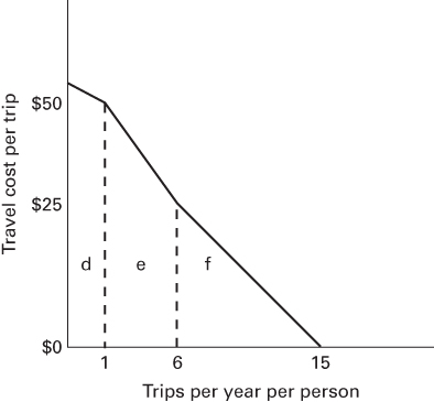
FIGURE 5.4 Demand Curve Derived from Travel-Cost Data
We can use this information to derive the demand curve shown in Figure 5.4, which plots the relation between travel cost and visits. With this demand curve in hand, total consumer surplus can be determined from the following formula:
The 1,000 people living in area A get a huge amount of surplus—the entire area under the demand curve, or in surplus from their 15 trips, and they incur no travel costs. Area B residents receive , but have to pay $25 of travel costs for each of their six trips. Finally, note that the folks from area C get very little net surplus (). They take only one trip and are almost indifferent toward going and not going.
Of course, in the real world, people are not identical—they have different incomes, tastes, and opportunity costs for travel. How do economists deal with these complications when applying the travel-cost method?
A study on the recreational benefits of Florida beaches for tourists provides a good example. The authors surveyed 826 tourists leaving Florida by plane or car and obtained information on the days spent at the beach and expenses incurred to use the beach, including hotel/motel or campground fees, meals, travel to and from the beach, and access fees and other beach expenses. They also gathered data on initial travel costs in and out of the state, length of stay, age, income, and perception of the crowds and parking conditions at the beaches. Their basic hypothesis was that, holding all the other factors constant, lower expenses in beach areas would lead tourists to spend a greater number of days at the beach.13
Using a statistical technique called multiple regression analysis, the authors were able to control all other factors and isolate the impact of expenses in beach areas on consumption. They found that demand was price inelastic, and a 10 percent increase in “price” led to only a 1.5 percent decrease in the time spent on the beach, all other things being equal. The average tourist spent 4.7 days on the beach, incurring an estimated daily expense of $85. With this information, the study estimated consumer surplus for all 4.7 days to be $179, for an average per day of $38. With 70 million tourist days per year, the authors calculated that Florida’s beaches yield a flow of value to tourists equal to $2.37 billion annually.
Evaluating the reliability of a travel-cost study boils down to determining how good a job the authors have done in controlling “other factors” that might affect recreation demand. For example, the beach study has been criticized because it did not control the opportunity cost of the tourists’ time. An extreme example shows why this might affect their result: Suppose that an idle playboy and a heart surgeon, in all other respects identical, were two of the tourists surveyed. Suppose further that hotel prices were lower in the area visited by the playboy, and he was observed to stay longer in the area and visit the beach more frequently. The incorrect inference would be that the lower prices caused the higher number of visits when, in fact, the surgeon simply could not afford to stay away from work.14
Another important external factor for travel-cost analysis is the presence of alternative recreational opportunities. In Figure 5.4, for example, suppose that some folks who lived in area C had access to a second, equally close forest. In that case, they might choose to travel to the original forest only every other year, thus shifting the observed demand curve in and reducing the measured surplus for all groups, C, B, and A. But the existence of this second, more distant forest would in fact have little impact on the actual surplus gained by folks in area A from visits to the original forest. The travel-cost method has been extended to address this type of issue as well.15
5.6 Measuring Benefits III: Hedonic Regression
Similarly to the travel-cost approach, the final method used for valuing nonmarket resources estimates benefits from observed market behavior. This method, hedonic regression, uses the change in prices of related (complementary) goods to infer a WTP for a healthier environment. The word hedonic means “pertaining to pleasure”; a hedonic regression estimates the pleasure or utility associated with an improved environment. As in the travel-cost method, regression techniques are used to hold constant factors that might be causing prices to change other than a degradation in environmental quality.
A good application of the hedonic regression method evaluated the damages arising from PCB contamination of sediments in the harbor of New Bedford, Massachusetts. The presence of PCBs was first made public in 1976; by 1983, about one-half the residents were aware of the pollution. Researchers attempted to measure the damage suffered in the community by examining the decline in real estate prices associated with the presence of this hazardous waste.
Their first step was to gather data on 780 single-family homes that had been sold more than once. The authors’ approach was to examine the relative decline in prices for those homes whose repeat sales spanned the pollution period, using regression techniques to control home improvements, interest rates, the length of time between adjacent sales for the same property, property tax changes, and per capita income in New Bedford. Assuming that knowledge of the pollution was widespread by 1982, houses located closest to the most hazardous area, where lobstering, fishing, and swimming were prohibited, had their prices depressed by about $9,000, with all other things being equal. Homes in an area of secondary pollution, where bottom fishing and lobstering were restricted, experienced a relative decline in value of close to $7,000.
Multiplying these average damage figures by the number of homes affected, the authors conclude that total damages experienced by single-family homeowners were close to $36 million. This estimate does not include the impact on renters or on homeowners in rental neighborhoods. Based on the results from this and other studies, firms responsible for the pollution have since paid at least $20 million in natural-resource damage claims.16
As with the travel-cost method, the key challenge in a hedonic regression study lies in controlling other factors that may affect the change in the price of the related good. The following section illustrates this difficulty when hedonic regression is used in its most controversial application: valuing human life.
5.7 The Value of Human Life
The most ethically charged aspect of benefit–cost analysis is its requirement that we put a monetary value on human life. I recall being shocked by the notion when I first learned of it in a college economics class. And yet, when we analyze the value of environmental improvement, we clearly must include reduction in human mortality as one of the most important benefits. If we seek to apply benefit–cost analysis to determine the efficient pollution level, we have no choice but to place a monetary value on life. Alternatively, if we adopt a safety standard, we can merely note the number of lives an action saves (or costs) and avoid the direct problem of valuing life in monetary terms.
And yet, because regulatory resources are limited, even the safety standard places an implicit value on human life. In the past, the U.S. Department of Transportation generally initiated regulatory actions only in cases where the implicit value of life was $1 million or more, the Occupational Safety and Health Administration employed a cutoff of between $2 million and $5 million, while the EPA used values ranging from $475,000 to $8.3 million.17 Courts also are in the business of valuing life when they award damages in the case of wrongful death. In the past, courts have often used the discounted future earnings that an individual expected to earn over his or her lifetime. This approach has some obvious flaws: it places a zero value on the life of a retired person, for example.
Efficiency proponents argue that the best value to be placed on life is the one people themselves choose in the marketplace. Hedonic regression can be used to estimate this value. By isolating the wage premium people are paid to accept especially risky jobs—police officer, firefighter, coal miner—it is possible to estimate the willingness-to-accept (WTA) an increase in the risk of death and, implicitly, the value of a life.
For example, we know from Table 5.1 that police officers face about a 1 in 10,000 chance of being killed by felons. Suppose that, holding factors such as age, work experience, education, race, and gender constant by means of regression analysis, it is found that police officers receive on average $700 more per year in salary than otherwise comparable individuals. Then, we might infer that, collectively, police officers are willing to trade $7 million (10,000 police times $700 per officer) for one of their lives. We might then adopt this figure of $7 million per life for use in estimating the environmental benefits of reducing risk and thus saving lives.
Note that this is not the value of a specific life. Most individuals would pay their entire income to save their own life or that of a loved one. Rather, the regression attempts to measure the amount of money the “average” individual in a society requires to accept a higher risk of death from, in our case, environmental degradation. For this reason, some economists prefer to call the measure the “value of a statistical life” instead of the “value of a life.” We use the latter term because the lives at stake are indeed quite real, even if they are selected from the population somewhat randomly. An overall increase in mortality risk does mean that human lives are in fact being exchanged for a higher level of material consumption.
Even on its own terms, we can identify at least three problems with this measure. The first is the question of accurate information: Do police recruits really know the increased odds of death? They might underestimate the dangers, assuming irrationally that it “won’t happen to me.” Or, given the prevalence of violent death on cop shows, they might actually overestimate the mortality risk. The second problem with this approach is sample selection bias. Individuals who become police officers are probably not representative of the “average” person regarding their preference toward risk. People attracted to police work are presumably more risk-seeking than the average person.
A third problem with applying this measure to environmental pollution is the involuntary nature of risk that is generated. In labor markets, people may agree to shoulder a higher risk of death in exchange for wages; however, people may require higher compensation to accept the same risk imposed upon them without their implicit consent. Polluting the water we drink or the air we breathe is often discussed in terms of violating “rights”; rights are typically not for sale, while labor power is. We will explore the issue of a “right” to a clean environment later, when we evaluate the safety standard in Chapter 7.
Hedonic regression researchers have attempted to control these factors as best they can. Reviews of wage–risk studies suggest that the median value for a statistical life in the United States or other wealthy countries is around $7 million. By contrast, studies conducted in Bangladesh place the value there at only $150,000. This huge discrepancy again reveals the moral choices implicit when using a consumer surplus (WTP or WTA) measure of value: because poor people have less income, they will be willing to accept riskier jobs at much lower wages. This means that reductions in the risk of death emerge in this benefit–cost framework as much less valuable to them.18
Using hedonic measures to value life thus raises a basic question: to what extent are labor market choices to accept higher risk really “choices?” Consider the following recent description of 12-year-old Vicente Guerrero’s typical day at work in a modern athletic shoe factory in Mexico City:
He spends most of his time on dirtier work: smearing glue onto the soles of shoes with his hands. The can of glue he dips his fingers into is marked “toxic substances . . . prolonged or repeated inhalation causes grave health damage; do not leave in the reach of minors.” All the boys ignore the warning.19
Vicente works at his father’s urging to supplement the family income with his wages of about $6 per day.
From one perspective, Vicente does choose to work in the factory. By doing so, he respects his father’s wishes and raises the family’s standard of living. However, his alternatives are grim. Vicente’s choices are between dying young from toxic poisoning or dying young from malnutrition. In important respects, Vicente’s choices were made for him by the high levels of poverty and unemployment that he was born into.
Similarly, the “choice” that a worker in a First World country makes to accept higher risks is also conditioned by general income levels and a whole variety of politically determined factors such as the unemployment rate and benefit levels, access to court or regulatory compensation for damages, the progressivity of the tax structure, social security, disability payments, food stamps and welfare payments, and access to public education and health-care services. All these social factors influence the workers’ alternatives to accepting risky work. By utilizing a hedonic regression measure for the value of life, the analyst is implicitly either endorsing the existing political determinants of the income distribution or assuming that changes in these social factors will not affect the measure very much.
Valuing life by the “acceptance” of risk in exchange for higher wages reflects the income bias built into any market-based measure of environmental benefits. The hedonic regression method values Vicente’s life much less than that of an American worker of any age simply because Vicente’s family has a vastly lower income. Proponents of this approach would argue that it is appropriate, because it reflects the real differences in trade-offs faced by poor and rich people. We will explore this issue further when we discuss the siting of hazardous waste facilities in Chapter 7. The point here is to recognize this core ethical dilemma posed by using hedonic regression to determine the value of life.
5.8 Summary
This chapter discussed the methods that economists use for valuing the nonmarket benefits of environmental quality. The focus has been on problems with such measures. Consider the questions an analyst has to answer in the process of estimating, for example, the benefits of PCB cleanup:
- Is consumer surplus a good measure of benefits, especially when valuing life?
- Which measure should be used: WTP or WTA?
- How reliable is the risk assessment?
- How broad a scope of benefits should be included?
- How precise and reliable are the benefit measures?
There simply are no generally accepted answers to any of these questions. A good benefit analyst can only state clearly the assumptions made at every turn and invite the reader to judge how sensitive the estimates might be to alternative assumptions.
Despite their many uncertainties, however, nonmarket estimates of environmental benefits are increasingly in demand by courts and policymakers. As environmental awareness has spread, claims for natural-resource damages are finding their way into courts more and more frequently. One important court decision confirmed the right to sue for nonuse-value damage to natural resources and explicitly endorsed the contingent valuation CV methodology as an appropriate tool for determining the existence or option value.20 In addition, policymakers require benefit estimates for various forms of benefit–cost analysis. As we discussed in the previous chapter, all new major federal regulations have been required to pass a benefit–cost test when such tests are not prohibited by law.
In an ambitious article in the journal Nature, an interdisciplinary group of scientists attempted to place a value on the sum total of global ecosystem services—ranging from waste treatment to atmospheric regulation to nutrient cycling.21 They concluded, stressing the huge uncertainties involved, that ecosystems provide a flow of market and nonmarket use value greater than $33 trillion per year, as against planetary product (world GDP) of $18 trillion!
The authors use many of the tools described in this chapter. In justifying their effort, they state, “although ecosystem valuation is certainly difficult and fraught with uncertainties, one choice we do not have is whether or not to do it. Rather, the decisions we make as a society about ecosystems imply valuations (although not necessarily in monetary terms). We can choose to make these valuations explicit or not . . . but as long as we are forced to make choices, we are going through the process of valuation.”22
Ultimately, economists defend the benefit measures on pragmatic grounds. With all their flaws, as the argument goes, they remain the best means for quantifying the immense advantages associated with a high-quality environment. The alternative, an impact statement such as the EIS to be discussed in Chapter 10, identifies the physical benefits of preservation in great detail but fails to summarize the information in a consistent or usable form.
At this point, benefit analysis is a social science in its relative infancy; nevertheless, it is being asked to tackle very difficult issues and has already had major impacts on public policy. Thousands of environmental damage studies have been completed in the last two decades. Perhaps, the wealth of research currently under way will lead to greater consensus on acceptable resolutions to the problems identified in this chapter.
KEY IDEAS IN EACH SECTION
- 5.0 There are both market and nonmarket benefits to environmental protection. Market benefits are measured at their dollar value; a value for nonmarket benefits must be estimated using economic tools.
- 5.1 The total value of an environmental benefit can be broken down into three parts: use, option, and existence values.
- 5.2 Economists consider the benefits of environmental protection to be equal to the consumer surplus gained by individuals through such environmental measures. For a freely provided public good, such as clean air or water, a consumer’s willingness to pay (WTP) for a small increase in the good or willingness to accept (WTA) a small decrease should be a good approximation to consumer surplus gained or lost. In actuality, however, the measured WTA is almost always substantially greater than the measured WTP. Prospect theory provides one explanation for the difference; a second explanation depends on the closeness of substitutes for the good in question.
- 5.3 Environmental risks must be estimated by means of epidemiological or animal studies. The estimated risk to humans varies depending on factors such as the assumed dose–response model. The risk to the population at large from an environmental hazard depends on both the toxicity of the pollutant and the number of people or animals exposed. Public perceptions of relative risk often differ from those based on scientific risk assessment. Among other factors, this may be due to a distrust of scientists, as well as risk aversion.
- 5.4 The first approach used for estimating nonmarket benefits is based on survey responses and is known as contingent valuation (CV). CV studies are controversial due to the possibility of free riding and strategic, hypothetical, and embedding biases. However, CV is the only available approach for estimating the benefits of environmental protection primarily based on existence value.
- 5.5 Another approach to estimating the nonmarket benefits is the travel-cost method, used principally for valuing parks, lakes, and beaches. Researchers construct a demand curve for the resource by relating the information about travel cost to the intensity of the resource use, holding all other factors constant.
- 5.6 The final method of measuring the nonmarket benefits of environmental protection is known as hedonic regression. This approach estimates the benefits of an improvement in environmental quality by examining the change in the price of related goods, holding all other factors constant.
- 5.7 Hedonic regressions that rely on the wage premium for risky jobs are used to place a monetary value on human life. This is often necessary if benefit–cost analysis is to be used for deciding the right level of pollution. This is a gruesome task; yet, even if regulators do not explicitly place a dollar value on life, some value of life is implicitly chosen whenever a regulatory decision is made. As a market-based measure, hedonic regression assigns a higher value of life to wealthier people, because their WTP to avoid risks is higher. This poses an obvious moral dilemma.
REFERENCES
- American Lung Association. 2009. State of the air. http://www.lungusa.org/about-us/publications/.
- Arrow, Kenneth, Robert Solow, Edward Leamer, R. Radner, and H. Schuman. 1993. Report of the NOAA panel on contingent valuation. Federal Register 58(10): 4201–614.
- Bell, Frederick, and Vernon Leeworthy. 1990. Recreational demand by tourists for saltwater beach days. Journal of Environmental Economics and Management 18(3): 189–205.
- Bishop, Richard C., and Michael P. Welsh. 1992. Existence value and resource evaluation. Unpublished paper.
- Boyle, Kevin J., and Richard C. Bishop. 1987. Valuing wildlife in benefit–cost analysis: A case study involving endangered species. Water Resources Research 23: 942–50.
- Bromley, Daniel. 1995. Property rights and natural resource damage assessments. Ecological Economics 14(3): 129–35.
- Carson, Richard. 2011. Contingent valuation: A comprehensive bibliography and history. Cheltenham, U.K.: Edward Elgar.
- Costanza, R., R. d’Arge, R. de Groot, S. Farber, M. Grasso, B. Hannon, K. Limburg, et al. 1997. The value of the world’s ecosystem services and natural capital. Nature 387(6630): 253–59.
- Freeman, A. Myrick III. 1985. Supply uncertainty, option price, and option value. Land Economics 61(2): 176–81.
- ______. 1993. The measurement of environmental and resource values: Theory and methods. Washington, DC: Resources for the Future.
- Glenn, Barbara S., J. A. Foran, and Mark Van Putten. 1989. Summary of quantitative health assessments for PCBs, DDT, dieldrin and chlordane. Ann Arbor, MI: National Wildlife Federation.
- Gough, Michael. 1989. Estimating cancer mortality. Environmental Science and Technology 8(23): 925–30.
- Horowitz, J., and K. McConnell. 2002. A review of WTA/WTP studies. Journal of Environmental Economics and Management, 44: 426–47.
- Johnson, Kevin. 2008. Police deaths plummet in first half of ’08. USA Today, 10 July, Page 1.
- Johnson, Laurie. 1999. Cost perceptions and voter demand for environmental risk regulation: The double effect of hidden costs. Journal of Risk and Uncertainty 18(3): 295–320.
- ______. 2003. Consumer versus citizen preferences: Can they be disentangled? Working paper, University of Denver.
- Kahneman, Daniel, and Amos Tversky. 1979. Prospect theory: An analysis of decisions under risk. Econometrica 47(2): 263–91.
- Kammen, Daniel, and David Hassenzahl. 1999. Should we risk it?: Exploring environmental, health, and technological problem solving. Rutherford, NJ: Princeton University Press.
- Khanna, Neha, and Duane Chapman. 1996. Time preference, abatement costs and international climate change policy: An appraisal of IPCC 1995. Contemporary Economic Policy 13(2): 56–66.
- Knetsch, Jack. 2007. Biased valuations, damage assessments, and policy choices: The choice of measurement matters. Ecological Economics, 63: 684–89.
- Knetsch, Jack, and Daniel Kahneman. 1992. Valuing public goods: The purchase of moral satisfaction. Journal of Environmental Economics and Management 22(1): 57–70.
- Kopp, Raymond J., Paul R. Portney, and V. Kerry Smith. 1990. Natural resource damages: The economics have shifted after Ohio v. United States Department of the Interior. Environmental Law Reporter 20: 10127–31.
- Mendelsohn, Robert, Daniel Hellerstein, Michael Huguenin, Robert Unsworth, and Richard Brazee. 1992. Measuring hazardous waste damages with panel models. Journal of Environmental Economics and Management 22(3): 259–71.
- National Cancer Institute. 2010. FactSheet. www.cancer.gov/cancertopics/factsheet/Tobacco/cessation.
- National Safety Council. 2010. http://www.nsc.org/news_resources/Documents/nscInjuryFacts2011_037.pdf.
- Putting a price tag on life. 1988. Newsweek, 11 January, 40.
- Shaw, W. Douglas. 1991. Recreational demand by tourists for saltwater beach days: Comment. Journal of Environmental Economics and Management 20: 284–89.
- Revesz, Richard and Michael A. Livermore. 2008. Retaking Rationality: How cost-benefit analysis can better protect the environment and our health. New York: Oxford University Press.
- Underage workers fill Mexican factories, stir U.S. trade debate. 1991. Wall Street Journal, 8 April.
- U.S. Environmental Protection Agency. 1990. Reducing risk: Setting priorities and strategies for environmental protection. Washington, DC: U.S. EPA.
- ______. 2010. What’s your EnviroQ? www.epa.gov/epahome/enviroq/index.htm#lungcancer.
- Value of intangible losses from Exxon Valdez spill put at $3 billion. 1991. Washington Post, 20 March.
- Viscusi, W. Kip. 2004. The value of life. In New Palgrave dictionary of economics and the law (2nd ed.) New York: Palgrave Macmillan.
- Wilson, Richard, and E. A. C. Crouch. 1987. Risk assessment and comparisons: An introduction. Science 236: 267–70.
APPENDIX 5A: WTA and WTP Redux
In Chapter 5, we noted that there is a large and persistent gap between people’s estimated WTP for environmental cleanup and their WTA compensation in exchange for environmental degradation. Two explanations have been offered for this. The first is prospect theory: people form an attachment to the status quo, and thus feel less strongly about cleanup than they do about degradation. A second explanation flows from conventional economic theory. It turns out, as this appendix shows, that when goods have few substitutes, WTA should be higher than WTP. We also review here the results of an interesting experiment that tried to sort out whether the observed WTA–WTP disparities are best explained by this “no good substitutes” argument, or prospect theory, and think a little more about why it matters.
5A.1: An Indifference Curve Analysis
Because this appendix is optional,1 we are going to assume that you perfectly recall how indifference curve analysis works from a previous course and jump right into the diagrams. Figure 5A.1 shows my (Eban’s) indifference curve map for standard quarters and one of the state quarter series, the one with Wyoming on the tail side. The curves are drawn in a straight line, implying that, to me, the goods are perfect substitutes, with a (marginal) rate of substitution of 1:1. I am not a coin collector, I just like money. So, I am equally as happy with four standard quarters and one Wyoming quarter as with one standard and four Wyomings.
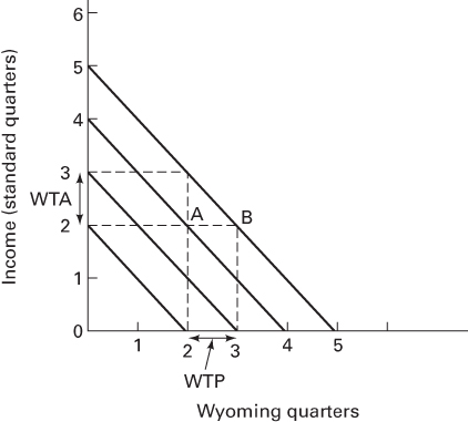
FIGURE 5A.1 WTA–WTP: Perfect Substitutes
Now, suppose that I am at point A (2, 2). What is my maximum WTP to get one more Wyoming and move to point B (3, 2)? The answer is illustrated by the distance marked WTP in the diagram; if I paid $0.25 to get to B, I would be just as well off as I was at A—paying anything less makes me better off. Therefore, $0.25 is my maximum WTP.
Let’s change the rules. Suppose that I am still at point A (2, 2). What is my minimum WTA to give up a chance to move to B (3, 2)? To be equally happy as I would have been at B, I need to be provide income until I am on the same indifference curve as B. But, that is the distance marked WTA on the diagram—again, one standard quarter or $0.25. When goods are perfect substitutes, WTA and WTP should be identical.2
In Figure 5A.2, the trading gets more serious. I am now confronted with a choice of spending money to reduce my risk of death: let’s say I can do this by laying out additional dollars each month on pesticide-free organic vegetables. On the horizontal axis, the risk of death gets more severe as we move toward the origin. For the purposes of illustration, let us also say that each additional $1 per month spent on pesticide-free veggies reduces my extra risk of dying by 1 out of 1 million.
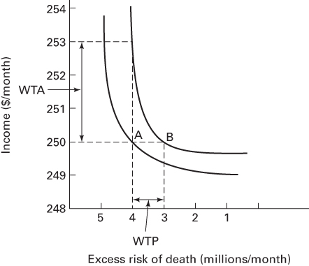
FIGURE 5A.2 WTA–WTP: Poor Substitutes
Note that these indifference curves are not straight lines; instead, they have the conventional bowed-in shape. The slope of the indifference curves decreases as risk levels decrease, reflecting a decreasing rate of marginal substitution. At high levels of risk, I am willing to trade a lot of income to reduce the risk a little. But, as my risk level decreases, I am less willing to accept cash in exchange for further safety. Put another way, at high risk levels, cash is not a good substitute for risk reduction.
As the diagram shows, when goods are not perfect substitutes, WTA will tend to be higher than WTP—a lot higher when the indifference curves are steeper, indicating poor substitutability. If I start at point A (with $250 per month and a 4 out of 1 million increased risk of death by pesticide consumption), then my maximum WTP to move to an excess risk of 3 out of 1 million is the line segment labeled WTP—equivalent to $1. By contrast, my minimum WTA compensation to stay at an excess risk level of 4 out of 1 million is illustrated on the income axis. To be just as content as I would have been at point B, I would have to be given enough cash to get me out to the higher indifference curve or $3. It is apparent from this diagram that WTA will generally be greater than WTP, and the difference increases as one moves along the horizontal axis toward the origin and higher risk levels.
5A.2: Prospect Theory or Substitutability?
A group of researchers had fun trying to sort out the explanation—prospect theory or poor substitutes—for the observed differences between WTA and WTP by performing experiments with a panel of college students. In the first experiment, the panel members were given an initial endowment of $3 and a small piece of candy. The researchers then conducted a series of trials to find out how much students would be WTP to upgrade to a brand-name candy bar. In an alternate series of experiments, different students were given the cash and the candy bar and then asked for their WTA cash to downgrade to the small piece of candy.3
The second experiment raised the ante: students were given $15 and a food product such as conventional deli sandwich, which, of course, bears a low risk of a possible infection from pathogens such as salmonella. Students were then asked how much they would pay to upgrade to a stringently screened food product with a very low risk of infection. In addition to hearing a bit about the symptoms of salmonella infection, they were provided with the following sort of information: “The chance of infection of salmonellosis is one in 125 annually. Of those individuals who get sick, one individual out of 1,000 will die annually. The average cost for medical expenses and productivity losses from a mild case of salmonella is $220.”
In the last stage of the experiment, the researchers flipped the property rights. This time, they gave the students the screened food product and the $15 and then asked their for WTA cash to downgrade to the conventional product. (In both cases, of course, the students actually had to eat the sandwiches!) Each subject participated in either both WTP experiments or both WTA experiments, but no individual was involved in WTP and WTA sessions. Finally, each of the 142 participants sat through several trials to allow them to gain experience with the experimental procedure.
In the candy bar experiment, WTA and WTP quickly converged very close to the market price of $0.50. However, for risk reduction, WTA remained well above WTP, even after 20 repeated trials. For exposure to salmonella, the mean WTA was $1.23, twice the WTP of $0.56. The authors concluded that this experiment, along with subsequent work, provides support for a “no good substitutes” explanation of the WTA–WTP discrepancy, as opposed to the one based on prospect theory. Do you agree?
Advocates of prospect theory might respond that candy bars or other low-value items do not provide a good test of the two theories: people are not likely to become attached to a candy bar or a coffee mug in the same way that they might become attached to a grove of trees in a local park. In this sense, the two explanations begin to converge. People are attached to the status quo because there are no good substitutes for environmental degradation from the status quo!
Regardless of the explanation, this experiment also illustrates that the choice of WTP or WTA in some sense flows naturally from the assignment of property rights. If people own the conventional sandwich, then it makes sense to ask for their WTP to upgrade; if they own the superior sandwich, then it is natural to ask for their WTA to downgrade.
REFERENCES
- Carlin, P. S., and Sandy, R. (1991), Estimating the Implicit Value of a Young Child’s Life. Southern Economic Journal 58(1), pp. 186–202.
- Hanneman, Michael. 1991. Willingness to pay and willingness to accept: How much can they differ? American Economic Review 81(3): 635–47.
- Shogren, Jason, Seung Y. Shin, Dermot Hayes, and James Kliebenstein. 1994. Resolving differences in willingness to pay and willingness to accept. American Economic Review 84(1): 255–70.