9
Cyber Modeling and Simulation and System Risk Analysis
“Cyber Risk,” the other side of the enabling technologies provides time‐saving conveniences that we have come to expect, has only recently added the word “risk.” Much like the safety engineering movement that arose after we came to expect automobiles to go at unprecedented speeds and distance (e.g. seat belts only became mandated in the 1970s), cyber is now moving toward prescriptive policies to ensure positive user experience. This quality vs. security question is pertinent to cyber, much as it was to the auto industry a generation ago. A new wrinkle with cyber, however, is the active agency of the perpetrator compromising software vulnerability; failure rates proportional to attacker’s skill.
9.1 Background on Cyber System Risk Analysis
Due to practitioners usually associating system “quality” with software quality (Ivers 2017), or verification of a system’s design and subsequent measures of performance, it is sometimes actually easier to design a testing regimen based on known vulnerabilities and level of interest in hacking them. While this is one instance of system quality, I believe that the more comprehensive quality concept that developed around both the product and process development in the automotive industry (National Academy of Engineering 1995) is the kind of thinking necessary to develop secure cyber products.
For example, looking at Figure 9.1’s Bathtub curve, both random and “wear out” failures are predictable for a given material with known characteristics. In addition, for consumer packaged goods manufacturing, the bathtub curve is a “rule of thumb” used for introducing any new product into the manufacturing process.
Figure 9.1 The bathtub curve – when and why of failures.
While Figure 9.1’s simple depiction of product life is an attractive mental model for any system in production, there are a few extra considerations for cyber systems (Table 9.1).
Table 9.1 Cyber modeling and the bathtub failure curve.
| Enterprise components and bathtub curve for cyber | Description |
| People | Attacker/defender skill are independent variables in determining system failure rate; whether an exploit succeeds |
| Policy/Process | Patching processes may lead to “windows of vulnerability,” adding discrete discontinuities to the constant failure rate section of the middle section of the bathtub curve |
| Process | Sampling is proportional to, and determinative of, knowledge acquisition on the part of both attackers and defenders; not a material depletion event stream |
| Technology | Lack of material/assembly failure that makes up much of the infant mortality section of the bathtub curve for manufacturing of consumer packaged goods, the foundation of the bathtub curve – cyber systems under inspection are assumed to work until they are decommissioned, or exploited |
One of the key differences between manufactured product lifecycles and cyber systems is the active perpetrator. In addition, separating the “wear out” from the “random” failures, in a non‐stationary environment, makes the situation much more challenging; requiring a baseline that essentially requires any kind of anomaly to be detected.
While a high‐level example of an attacker is provided in Figure 3.7 (Chapter 3), taking it up a level, and consequent to improving cyber security, is including cyber security into project management’s nexus of systems engineering and project planning (Kossiakoff et al. 2011), as shown in Figure 9.2.
Figure 9.2 Systems engineering and project management for preventive cyber security.
As shown in Figure 9.2, systems engineering and project planning, done jointly, are required for preventing cyber anomalies in the first place. In addition, while the International Standards Organization published ISO 31000 to handle risk, the standard needs to be tailored for use in the cyber domain. This often includes looking at the overall system, its context, or reasons for particular construction, and how an attacker might look at the system. Fortunately, most systems have the common “V” construction (Figure 9.3), resulting in metrics being assigned at each of the respective construction phases.
Figure 9.3 The “V” model of systems engineering.
As discussed in Table 9.3, there are multiple security metrics available for evaluating systems, depending on how much we know. The assumption here is that cyber system evaluation is a black box analysis, with little known about the system, where a general, time‐based approach works as a first‐order analysis.
9.2 Introduction to using Modeling and Simulation for System Risk Analysis with Cyber Effects
A methodology that evaluates pre‐event cyber security risks, based on an enterprise’s People, Processes, and Tools (PPT), is proposed here to proactively secure critical information that compose a company’s technical and management differentiators. The “people” part of cyber vulnerability, well‐known as the most common threat vector, is a challenge to model.
One example of risk evaluation is “war gaming” cyber, via M&S. This naturally brings to mind attackers/defenders. Cyber is novel in that it has at least one more dimension than standard games – team members, insiders, may be a source of risk. Some insider attack scenarios (Serdiouk 2007) are shown in Table 9.2.
Table 9.2 Internal threat scenario examples.
| Threat scenario | Description |
| 1 | Insiders who make “innocent” mistakes and cause accidental disclosures. Probably the most common source of breached privacy. For example, overheard hall conversations, misclassified data, email, etc. |
| 2 | Insiders who abuse their record access privileges. Individuals that have access to data and violate the trust associated with that access. |
| 3 | Insiders who knowingly access information for spite or for profit. When an attacker has authorization to some part of the system, but not to the desired data and gains access to that data by other means. |
| 4 | The unauthorized physical intruder. The attacker has physical entry to points of data access but has no authorization to access the desired data. |
| 5 | Vengeful employees and outsiders, such as vindictive patients or intruders, who mount attacks to access unauthorized information, damage systems, and disrupt operations. |
Table 9.2’s “people” threats may be some of the most challenging to handle, due to the perpetrators already being inside the initial security perimeters designed to keep out external threats. Technical and operational scenarios (Chapter 4, Table 4.3) will overlap with Table 9.2’s examples, in that applying critical security controls (CSCs [Chapter 12]) should protect from obvious threats, with training to maintain both awareness and responsiveness to cyber threats.
Leveraging widely used availability estimations, common to manufacturing, we will provide an approach for estimating failure rates for the respective PPT domains and combine them into an overall exploit estimation model. This approach’s flexibility results in quick estimation of how countermeasures will contribute to increases in system cyber security.
9.3 General Business Enterprise Description Model
Evaluating a system’s availability for mission performance, a solved problem for manufacturing quality control, is currently an issue in assessing IT and cyber physical system risk. Leveraging known systems engineering concepts, from data analysis to modeling mean time to failure (MTTF), provides cyber security designers with modeling and simulation (M&S) tools to describe and evaluate the people, process and technology (PPT) domains that compose a modern information‐based enterprise. In addition, organizing these quality control techniques with entity‐relational methods provides tools to coordinate data and parameterize enterprise evaluation models (Couretas 1998a, b). Similarly, Model‐Based Systems Engineering (MBSE [Friedenthal et al. 2011]), an entity‐relational approach for system description, is being used by the Department of Defense’s (DoD) Defense Information Services Agency (DISA) to build the Joint Information Environment (JIE), or future cross‐service network. Similarly, this approach applies to overall enterprise cyber risk evaluation (Couretas 2014).
DISA uses MBSE as a top‐down approach to design the JIE. We propose a similar approach, in using an MBSE‐like structure, to describe “as is” enterprises, modeling the respective PPT domains in terms of their “attack surfaces” (Manadhata and Wing 2008), with security metrics specified based on system/component vulnerabilities of interest (Table 9.3).
Table 9.3 Example security metrics.
| Security metric | Examples | |
| Core | CVSS | Common Vulnerability Scoring System is an open standard for scoring IT security vulnerabilities. It was developed to provide organizations with a mechanism to measure vulnerabilities and prioritize their mitigation. There has been a widespread adoption of the CVSS scoring standard within the information technology community. For example the US Federal government uses the CVSS standard as the scoring engine for its National Vulnerability database (NVDa) |
| TVM | Total Vulnerability Measure is an aggregation metric that typically doesn't use any structure or dependency to quantify the security of the network. TVM is the aggregation of two other metrics called the Existing Vulnerabilities Measure (EVM) and the Aggregated Historical Vulnerability Measure (AHVM). | |
| Probability (Attack‐Graph) | AGP | In Attack Graph‐based Probabilistic (AGP) each node/edge in the graph represents a vulnerability being exploited and is assigned a probability score. The score assigned represents the likelihood of an attacker exploiting the vulnerability given that all pre‐requisite conditions are satisfied. |
| BN | In Bayesian network (BN) based metrics the probabilities for the attack graph is updated based on new evidence and prior probabilities associated with the graph. | |
| Structural (Attack‐Graph) | SP | The Shortest Path (SP) (Ortalo et al. 1999) metric measures the shortest path for an attacker to reach an end goal. The attack graph is used to model the different paths and scenarios an attacker can navigate to reach the goal state which is the state where the security violation occurs. |
| NP | The Number of Paths (NP) (Ortalo et al. 1999) metric measures the total number of paths an attacker can navigate through in an attack graph to reach the final goal, which is the desired state for an attacker. | |
| MPL | Mean of Path Lengths (MPL) metric (Li and Vaughn 2006) measures the arithmetic mean of the length of all paths an attacker can take from the initial goal to the final goal in an attack graph. | |
| Time Based (General) | MTTR | Mean Time to Recovery (MTTR) (Jonsson and Olovsson 1997) measures the expected amount of time it takes to recover a system back to a safe state after being compromised by an attacker. |
| MTTB | Mean Time to Breach (MTTB) (Jaquith 2007), represents the total amount of time spent by a red team to break into a system divided by the total number of breaches exploited during that time period. | |
| MTFF | Mean Time to First Failure (MTFF) (Sallhammar et al. 2006) corresponds to the time it takes for a system to enter into a compromised or failed state for the first time from the point the system was first initialized. | |
a NVD has a repository of over 45 000 known vulnerabilities and is updated on an ongoing basis (National Vulnerability Database 2014).
Table 9.3’s metrics for core, attack graph, and temporal security evaluations give the system evaluator an “outer bound” of the system’s current security state, providing a rough guide for tailoring the domain‐based threat vectors for more specific evaluation(s). Using domains to narrow the scope for specific threat vectors results in the ability to estimate risk within individual domains. For example, estimating a “failure rate” for a sample population describes how long it will take for an exploit to occur (i.e. mean time to exploit [MTTE], tMTTE), for either an individual domain (e.g. People1/Process/Technology) or, in combination, for the overall enterprise (Figure 9.4).

Figure 9.4 Enterprise security view – people, process, and technology domains.
As shown in Figure 9.4, the security view for an enterprise decomposes into example PPT domains. Within each domain are the individual elements that compose the domain’s attack surface; characterized by an example exploit probability, λndt, for a given slice of time, dt. In this case, each domain’s attack surface is characterized by individual domain exploit rates, λn, and their combinations, (fi*fj).
9.3.1 Translate Data to Knowledge
The goal, as exemplified in Figure 9.5, is to evaluate/audit risk of an organization, and develop a report for leadership to understand where they stand, in terms of current cyber vulnerabilities.

Figure 9.5 Audit timeline – people/process/technology evaluation.
As shown in Figure 9.5, people, policies, processes and tools that compose the enterprise are periodically evaluated via surveys and interviews (i.e. “collectibles”) (Table 9.4).
Table 9.4 Enterprise evaluation – areas and time periods.
| Evaluation areas | Collectables | Time periods |
| People | Anomaly detection | Weeks – months |
| Policy/Process | Performance changes | Months – quarters |
| Tool/Technology | Allowed on network (e.g., white listing) | Hours – days |
In addition, Figure 9.5’s surveyed areas are the data used to develop a description of the enterprise’s interconnections and vulnerabilities (Figure 9.6).
Figure 9.6 Enterprise connections (people/policy/process/technology) and COA planning.
While Figure 9.6 brings out the input/output description of the respective enterprise domains, we will use the system’s entity‐relationship model, called a System Entity Structure (SES), to build a taxonomy‐like structure for describing the overall system. Using the people, processes, and technologies that make up the enterprise, use failure rate estimations for each domain, and in combination, to understand the current system’s MTTE. Given the above enterprise security description, we use combinations of Policy/Training/Technology to construct alternative strategies. For example, gathering the data, as shown in Figure 9.9, is stored in a SES to provide an overall enterprise model to be exercised for risk/vulnerability of the system in question (Figure 9.7).
Figure 9.7 Question & answer process (Q&A) for system entity structure (Ontology) development.
As shown, Figure 9.7 leverages the SES (Zeigler et al. 2000) as the enterprise “As Is” Graph Description to organize disparate People/Processes/Tools descriptions:
- Tree Structure example is currently an “AND” graph, where each of the decomposed entities has its own failure rate, that is used to contribute to the overall failure rate for each key node of the Enterprise (e.g. PPT).
- Decompositions can also include “OR” specialization nodes, where alternative people, process, or technology implementations are available.
- Graph Structure is formally called a System Entity Structure; used to describe an enterprise for evaluation (Couretas 1998a, b).
An example questionnaire, filled out to check the vulnerability of an enterprise network, is provided in Table 9.5.
Table 9.5 People/policy/process/technology example breakdown (vulnerability analysis).
| People | Policy | Process | Technology | ||
| Weaknesses | Access, Associations, and adherence | Locations, suppliers, and servicing | Software updates, service times, and maintenance | Access, connectivity, and storage | |
| Crit Info Access | Login/password | Connection via servicing | |||
| Vulnerability | Personal issues | Adherence issues | SANS 20 controls/compliance | ||
| Units | Enterprise | Risk, No. weaknesses, Vulnerabilities, Critical information access | |||
| Components | Entities, relations | Rules | Timing | Facts | |
| Equations | Enterprise | Risk = 1 – Πi(1 – ri) ∣ i = framework component, r = component risk with the risk for each component being – Risk = 1 – (weaknesses/(weaknesses + critical information access)) | |||
| Components | People have access and associations, which are represented in an entity‐relation diagram; static. System Accesses (X) and external communications (Y) are determined by user base |
Policy constrains accesses and associations, Policy prescribes system behavior (S) and determines how users are allowed to interact (δext) with the system |
Discrete Event System (DEVS) Model for process representation: M = { X, Y, S, ta, δext, δint, λ} where {X,Y} = MEs and Si = IEs (enables dynamic simulation) (Zeigler) | Manadhata defines a technical attack surface as the triple, {MEs, CEs, Ies}, where MEs is the set of entry points and exit points (X,Y), CEs is the set of channels and IEs is the set of untrusted data items of s. In DEVS, Si = IEs | |
| Tools | Enterprise | Analytic Hierarchy Process (AHP) (e.g. Checkmate) | |||
| Components | Link Analysis (e.g., Palantir, i2, etc.) | “Playbooks” | Visio, power point, JIRA | CERT – known exploits | |
Figure 9.8 provides an example of how the failure rates (e.g. λ) are rolled up for the respective PPT/technology vulnerabilities.
Figure 9.8 Enterprise model and parameterization.
As shown in Figure 9.8, λ is the failure rate for each respective domain (e.g. people, processes, tools/technologies), or one of its components. Representing each of the people/process/tools with an exponential distribution results in an “additive” combination of failure rates, leveraging the Palm‐Khintchine Theorem, to develop a “model” over the heterogeneous data for the respective domains.
9.3.2 Understand the Enterprise
Figure 9.7 provides a data discovery process that uses the well‐known knowledge‐engineering approach2 of interviews, surveys,3 and automated tools to collect data about an information processing enterprise. Data is then structured into domains, separated, and characterized by their estimated exploit rate. Given the respective exploit rates for each domain, these “models,” are then combined (e.g. via convolution) to estimate the MTTE (tMTTE).
Cyberattack data, getting better from authoritative sources in terms of attacks/vulnerabilities, are also available via surveys and interviews for tailored evaluation of information systems. Figure 9.9 provides an end‐to‐end process for translating interview data to failure rate “models” used to estimate vulnerability for a system of interest, providing an enterprise cyber risk estimate at one instant in time.
Figure 9.9 Data to strategy evaluation.
Figure 9.9’s approach, in developing models from collected data, is organized via an entity‐relationship model (i.e. SES).
9.3.3 Sampling and Cyber Attack Rate Estimation
Estimating a distribution for tmtte is a challenge due to the lack of data. Manufacturing quality, for example, only started to improve after the adoption of statistical process control techniques. The opacity of cyberattack/exploit data therefore presents a counting problem for developing model‐based approaches.
An ongoing assumption, here, is that at least some cyberattacks are undetected, and can go on, for some time. For example, the Ponemon Institute (The Ponemon Institute, LLC 2014) shows how 2/3 of system administrators have a challenge defining risk/vulnerability. In addition, Mandiant (2014) estimates up to 250 days before attacks are discovered within a system. We are therefore dealing with a random, unknown, attack, and detection process.
9.3.4 Finding Unknown Knowns – Success in Finding Improvised Explosive Device Example
One approach to measuring unexpected attack frequency, pioneered by the US Marines in 2005–2007 while encountering improvised explosive devices (IEDs) in Western Iraq, is the “find rate” of pre‐detonation IEDs. This includes counting the number of IEDs handled by Explosive Ordnance Detail (EOD) teams found through general reporting, and using this larger number in the denominator of a ratio that included unexpected attacks (Equation 9.1).

Equation 9.1: Pre‐detonation IED find rate (practical application from Iraqi Theater of Operations, 2006).
I believe a similar approach can be used to evaluate both the exploit rate for cyberattacks and, conversely, the success rate due to different attack mitigation strategies (Equation 9.2).
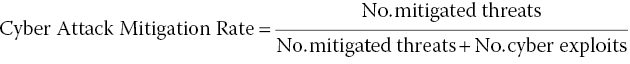
Equation 9.2: Cyberattack mitigation rate.
Looking at Equation (9.2), the Cyber Attack Mitigation Rate leverages all of the general effects of annual employee training, implementing new security processes, software patching, etc. in the number of mitigated threats. The number of cyber exploits, more challenging to count, is believed to be much less than the number of mitigated threats; simply due to the culture of trust that results in day‐to‐day use of the Internet by over 1 billion people. This leads us to believe that
Describing cyber exploits with small sample statistics (e.g. Poisson, etc.) therefore becomes an option for this initial estimate.
9.4 Cyber Exploit Estimation
While sample sizes for cyber exploits are a challenge to count, small sample statistics provide us with baseline models, and a theoretical underpinning, to start our inquiry. The model‐based approach proposed here will accommodate any phenomenological description (e.g. binomial, normal, etc.).
Data on cyberattacks is a challenge to get. Commercial attacks (e.g. Target, Nieman Marcus, etc.) make the news while the average consumer buys books on‐line, uses her credit card multiple times per day, and logs on to the Internet for both business and personal use.
In addition, most of the respected data sources on cyberattacks consist of reports or surveys. An example of the current state of available data is a recent report on Insider Threat (The Ponemon Institute, LLC 2014). The report focuses on privileged users (e.g. DB Admins, Network Engineers, etc.) using their assigned permissions beyond the scope of their assigned role. Data from 693 respondents, collected on a Likert scale, resulted in percentages – an example being “47% see social engineering of privileged users as a serious threat for their network’s exploitation …” While this is good, general, information, it lacks the granularity required for developing behavioral models that can be used for prediction and model‐based control; models with established base rates from available samples.
Seeing the human as a key component of any situational awareness evaluation, one approach to SA is shown in Table 9.6.
Table 9.6 Situational awareness (SA) – levels and indicators.
| Level | Time period | Indicator(s) |
| Strategic | Months – quarters | Anomaly detection |
| Tactical/Operational | Weeks – months | Process adherence |
| Technical | Hours – days | SIEM monitoring |
Combining Table 9.6’s insight with a model‐based approach provides a wrap‐up technique for evaluating overall risk, in potentially real‐time, to match the Δt of the attack surface. This includes using the rare event nature of exploits and convert this into an exploit rate for people, processes, and technology. Leveraging the Poisson distribution, for this initial estimate, the probability of exploit over the time period (t, t + dt], is λdt, and the probability of no exploit occurring over (t, t + dt] is 1° – °λdt.
Next, consider our outcome variable Yt as the number of events, or exploits, that have occurred in the time interval of length h. For such a process, the probability that the number of exploits occurring in (t, t + h] is equal to some value y ∈ {0, 1, 2, 3, …} is:
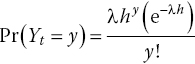
Equation 9.3: Poisson process.
Equation (9.3) is what is known as a Poisson process; events occur independently with a constant probability equal to λ times the length of the interval (that is, λh).
For a large number of Bernoulli trials, where the probability of an event in any one trial is small, the total number of events observed will follow a Poisson distribution. In addition, the “rate” can also be interpreted as the expected number of events during an observation period t. In fact, for a Poisson variate Y, E(Y) = λ. As λ increases, several interesting things happen
- The mean/mode of the distribution gets bigger.
- The variance of the distribution gets larger as well. This also makes sense: since the variable is bounded from below, its variability will necessarily get larger with its mean. In fact, in the Poisson, the mean equals the variance (that is, E(Y) = Var(Y) = λ).
- The distribution becomes more Normal‐looking (and, in fact, becomes more Normal).
While the Poisson process provides a flexible baseline to initially model our exploit rates, we use Figure 9.10, expanding on Figure 9.4, to provide an entity‐relational structuring for each domain’s descriptive data (e.g. exploit rates).
Figure 9.10 Enterprise vulnerability – exploit rates by domain.
9.4.1 Enterprise Failure Estimation due to Cyber Effects
Figure 9.10’s SES, similar to a SysML structure, is used for enterprise design (Couretas 1998a, b) and is a general structuring that provides both visual enterprise decomposition and a means to organize system data described by any distribution.
Exponential Distribution provides a rough approximation to Enterprise security failure. Advantages include:
- Get the conversation started about enterprise security structure (i.e. SES of Enterprise).
- Initial cut at Enterprise risk model (i.e. more accurate approaches available as data quality increases).
- Leverage well‐known mean time to failure for cyber domain.
- Cyber Risk Estimation = Mean Time to Exploit (MTTE)
Equation 9.4: Mean time to exploit (MTTE.)
Figure 9.11’s example uses 50% as an example marker; providing modeled enterprise with an approximately 2‐month MTTE.

Figure 9.11 Mean time to exploit example.
9.5 Countermeasures and Work Package Construction
One of the benefits of Equation (9.4)’s general representation is the ability to evaluate Policy, Training, and Technology options/strategies as potential countermeasures to system threats and vulnerabilities (Table 9.7).
Table 9.7 Example countermeasures as work packages.
| Packages/domain and work package | Cyber enterprise domain affected by work packages | Work package time/cost estimate | ||||
| Work packages | People (λpeople) | Process (λprocess) | Tool (λtool) | Implementation time | Cost ($ K) | |
| Policy | Access | • | ◦ | ◦ | Months | 10’s |
| Mobile device | • | • | • | Months | 10’s | |
| Critical information | • | • | ◦ | Months | 10’s | |
| Phishing | • | ◦ | ◦ | Weeks | 10’s | |
| Training | Internet use | • | ◦ | ◦ | Weeks | 10’s |
| Social engineering | • | • | ◦ | Weeks | 10’s | |
| Firewalls | ◦ | • | • | Days | 100’s | |
| Technology | M&C | ◦ | ◦ | • | Days | 100’s |
| Authentication | • | ◦ | • | Weeks | 100’s | |
As shown in Table 9.7, policy/training/technology countermeasures are relatively simple to evaluate in terms of their cost/time to implement, and their estimated effectiveness, using Equation (9.4)’s MTTE as a measure of effectiveness. The Policy/Training/Technology countermeasure therefore becomes a discount on the estimated PPT attack rate, as shown in the following equation:
Equation 9.5: Mean time to exploit (MTTE)(2).
- MTTE: Mean time to exploit
- D: Discount factor due to policy/training/technology countermeasure
- λvulnerability: People/Process/Tool estimated exploit rate
- t: Time
This model is then used to evaluate candidate countermeasures (e.g. policy, training, technology, etc.) in terms of systems engineering measures (e.g. time, quality, cost, etc.) for extending the MTTE (tMTTE). We can use this construct to evaluate work packages as countermeasures for their discrete (i.e. one‐time fix) and continuous learning curve contribution. In addition, this can be complemented by a look at Threat Pathway system representation (Nunes‐Vaz et al. 2014), and subsequent threat maturity estimation (e.g. using the beta distribution to estimate either threat or countermeasure development time), as an approach for estimating emerging threats.
9.6 Conclusions and Future Work
Using the SES‐based system representation, we can evaluate current people/process/tool remedies for given threats and determine how to segment an enterprise description using layered representations (e.g. deter, deny, etc.) with MTTE for pre‐event risk. In addition, we can extend this approach to post‐event considerations that include evaluating resilience and subsequent mean time to repair, along with an overall mission system Availability estimate with both pre‐ and post‐event risk evaluation.
Future work, therefore, includes both technical and management tools for evaluating systems for cyber security. Model‐based approaches capture management best practices in recently developed technologies. One example includes the expanding on current security information and event management (SIEM) systems with automatic controls’ responses, similar to what Canada’s DRDC is developing with their ARMOUR framework (DRDC (Canada) 2014a, b). Management evaluation of cyber systems includes expanding on MTTE‐based approaches for getting an architectural view of the current landscape of cyber risks and estimating how to systematically optimize the cost of security investments.4
Real‐time approaches, such as streaming analysis (Streilein et al. 2011), develop and the discrete distributions that describe patterns of behavior, using them as a form of a model to perform anomaly detection for the enterprise. Table 9.8 provides two examples of deep packet inspection platforms.
Table 9.8 Deep packet inspection platform examples (Einstein and SORM).
| System | Objective | Country | Source |
| System for Operative Investigative Activities (SORM) | Monitor all communications around the Sochi Olympics (e.g. including deep packet inspection for monitoring/filtering data) SORM‐1 intercepts telephone traffic, including mobile networks; SORM‐2 monitors Internet communication, including VoIP (Voice over Internet Protocol) programs like Skype; and SORM‐3 gathers information from all types of communication media. |
Russia | http://en.wikipedia.org/wiki/SORM http://www.theguardian.com/world/2013/oct/06/sochi‐olympic‐venues‐kremlin‐surveillance http://themoscownews.com/russia/20130671/191621273.html |
| EINSTEIN | EINSTEIN is an intrusion detection system (IDS) for monitoring and analyzing Internet traffic as it moves in and out of United States federal government networks. EINSTEIN filters packets at the gateway and reports anomalies to the United States Computer Emergency Readiness Team (US‐CERT) at the Department of Homeland Security. Einstein 1 (2006) – analyzes network flow information to provide a high‐level view for observing potential malicious activity. Einstein 2 (2008) – automated system that incorporates intrusion detection based on custom signatures of known or suspected threats. Einstein 3 (2013) – detects malicious traffic on government networks and stops that traffic before it does harm. |
USA | http://gcn.com/Articles/2013/07/24/Einstein‐3‐automated‐malware‐blocking.aspx?Page=2 http://searchsecurity.techtarget.com/definition/Einstein |
Each of the architectures in Table 9.8 include three layers in developing greater resolution for their inspection activities. These approaches would be complemented by using a model‐based approach that decomposes the enterprise into domains, with each domain represented by probability distributions, lending the overall system to the implementation of model‐based control. State observers (Luenberger 1979), often used in the energy domain, are implemented via “Luenberger Observers” to monitor natural gas line networks for detecting and reporting on anomalous pressure changes, assisting operators in pinpointing the location of a leak or breakage in a gas line network that can easily span thousands of miles. A similar approach can be used for cyber.
While employing a state observer at the network level is currently an aspirational goal, the work here provides a baseline in terms of
- representative distributions for exploit phenomena
- a method of organizing known problem data via entity‐relational hierarchy and
- a technique for combining the respective domain descriptions into a single, strategic, measure for whole of enterprise evaluation.
Leveraging contemporary systems and software tools, including MBSE, DEVS, and classical probability to provide a state observer for monitoring and controlling multiple attack surfaces will be a step forward in overall cyber security. For example, manufacturing quality control, once a problem in the “too hard” bucket due to the multiple people/process/technology dimensions in the physical domain, is now a solved problem. Similarly, this approach provides a path forward for managing and controlling the multiple people/process/technology dimensions in the logical domain.
9.7 Questions
- 1 How do the standard four risk approaches (e.g. avoid, accept, transfer, and mitigate) apply to cyber?
- 2 What additional domains (i.e. beyond People, Processes and Technology (PPT)) help with demonstrating a “complete” attack surface?
- 3 How are mobile and dormant devices included in an attack surface description?
- 4 Why does Equation (9.4) work for current cyber terrain?
- 5 What does the FAIR Institute’s Factor Analysis of Information Risk Model cover, in terms of the protected system?
- 6 Why are small sample statistics adequate for cyber modeling? What are the drawbacks?
- 7 How might work packages be constructed for countermeasure estimation in defensive cyber planning?