10
Dimension reduction in high‐dimensional multivariate time series analysis
The vector autoregressive (VAR) and vector autoregressive moving average (VARMA) models have been widely used to model multivariate time series, because of their ability to represent the dynamic relationships among variables in a system and their usefulness in forecasting unknown future values. However, when the number of dimensions is very large, the number of parameters often exceeds the number of available observations, and it is impossible to estimate the parameters. A suitable solution is clearly needed. In this chapter, after introducing some existing methods, we will suggest the use of contemporal aggregation as a dimension reduction method, which is very natural and simple to use. We will compare our proposed method with other existing methods in terms of forecast accuracy through both simulations and empirical examples.
10.1 Introduction
Multivariate time series are of interest in many fields such as economics, business, education, psychology, epidemiology, physical science, geoscience, and many others. When modeling multivariate time series, the VAR and VARMA models are possibly the most widely used models, because of their capability to represent the dynamic relationships among variables in a system and their usefulness in forecasting unknown future values. These models are described in many time series textbooks including Hannan (1970), Hamilton (1994), Reinsel (1997), Wei (2006), Lütkepohl (2007), Tsay (2013), Box et al. (2015), and many others.
Let Zt = [Z1,t, Z2,t, …, Zm,t]′, t = 0, ± 1, ± 2, …, be a m‐dimensional jointly stationary real‐valued vector process so that E(Zi,t) = μi is constant for each i = 1, 2, …, m and the cross‐covariances between Zi,t and Zj,s, E(Zi,t − μi)(Zj,s − μj), for all i = 1, 2, …, m and j = 1, 2, …, m, are functions only of the time difference (s − t). A useful class of vector time series models is the following vector autoregressive moving average model of order p and q, shortened to VARMA(p,q),
where Φp(B) = Φ0 − Φ1B − ⋯ − ΦpBp and Θq(B) = Θ0 − Θ1B − ⋯ − ΘqBq are autoregressive and moving average matrix polynomials of order p and q, respectively, Φi and Θj are nonsingular m × m matrices, and at is a sequence of m‐dimensional white noise processes with mean zero vector and positive definite variance–covariance matrix ε. Since one can always invert Φ0 and Θ0, and combine them into ε, with no loss of generality, we will assume in the following discussion that Φ0 = Θ0 = I, the m × m identity matrix. Furthermore, any VARMA model can be approximated by a vector AR model, in practice, one often uses the following vector autoregressive model of order p, shortened to VAR(p),
or
where the zeros of |I − Φ1B − ⋯ − ΦpBp| lie outside of the unit circle or, equivalently, the roots of |λpI − λp − 1Φ1 − ⋯ − Φp| = 0 are all inside of the unit circle. With no loss of generality, in the following discussion, we will mostly use the VAR(p) model with zero mean for our illustrations.
With the development of computers and the internet, we have had a data explosion. For a m‐dimensional multivariate time series, m being numbered in the hundreds or thousands is very common. If we simply consider m = 100, a simple VAR(2) model has a minimum of 2(100 × 100) = 20,000 parameters. For observations obtained yearly, we cannot estimate the model parameters, even with a hundred years of data.
To solve this problem, after introducing some existing methods, we will suggest the use of aggregation as a dimension reduction method, which is very natural and simple to use. We will compare our proposed method with other existing methods in terms of forecast accuracy through both simulations and empirical examples. The chapter will be organized as follows. Section 10.2 introduces and discusses several existing methods to handle high‐dimensional time series. The proposed procedure is introduced in Section 10.3. Monte Carlo simulations and empirical data analysis are presented in Sections 10.4 and 10.5, respectively. Lastly, further discussions and remarks are given in Section 10.6.
A condensed version for the first five sections of this chapter was presented in an invited talk at the 2017 ICSA (International Chinese Statistical Association) Applied Statistical Symposium in Chicago when the organization celebrated its 30th year anniversary. For a formal paper, please see Wei (2018). The supplementary appendix at the end of the chapter is from Li and Wei (2017).
10.2 Existing methods
In this section, we briefly review the existing methods that handle time series modeling in high‐dimensional settings, including various regularization methods (Section 10.2.1), the space–time STAR model if the data is collected from different locations (Section 10.2.2), model‐based clustering (Section 10.2.3), and the factor model (Section 10.2.4).
10.2.1 Regularization methods
Let Zt = [Z1,t, Z2,t, …, Zm,t]′, t = 1, 2, …, n, be a zero‐mean m‐dimensional time series with n observations. It is well known that the least squares method can be used to fit the VAR(p) model by minimizing

where ‖‖2 is Euclidean (L2) norm of a vector. In practice, more compactly, with data Zt = [Z1,t, Z2,t, …, Zm,t]′, t = 1, 2, …, n, we can present the VAR(p) model in Eq. (10.2) in the matrix form,
where

and
So, minimizing Eq. (10.3) is equivalent to
where ‖‖F is the Frobenius norm of the matrix.
For a VAR model in high‐dimensional setting, many regularization methods have been developed, which assume sparse structures on coefficient matrices Φk and use regularization procedure to estimate parameters. These methods include the Lasso (Least Absolute Shrinkage and Selection Operator) method, the lag‐weighted lasso method, and the hierarchical vector autoregression method, among others.
10.2.1.1 The lasso method
One of the most commonly used regularization methods is the lasso method proposed by Tibshirani (1996) and extended to the vector time series setting by Hsu et al. (2008). Formally, the estimation procedure for the VAR model is through
where the second term is the regularization through L1 penalty with λ being its control parameter. λ can be determined by cross‐validation. The lasso method does not impose any special assumption on the relationship of lag orders and tends to over select the lag order p of the VAR model. This leads us to the development of some modified methods.
10.2.1.2 The lag‐weighted lasso method
Song and Bickel (2011) proposed a method that incorporates the lag‐weighted lasso (lasso and group lasso structures) approach for the high‐dimensional VAR model. They placed group lasso penalties introduced by Yuan and Lin (2006) on the off‐diagonal terms and lasso penalties on the diagonal terms. More specifically, if we denote Φ(j, − j) as the vector composed of off‐diagonal elements {ϕj,i}i ≠ j, and Φk(j, j) as the jthdiagonal element of Φk, then the regularization for Φk is

where W(−j) = diag(w1, …, wj − 1, wj + 1, …, wm), an (m − 1) × (m − 1) diagonal matrix with wj being the positive real‐valued weight associated with the jth variable for 1 ≤ j ≤ m, which is chosen to be the standard deviation of Zj,t. λ is the control parameter that controls the extent to which other lags are less informative than its own lags. The first term of Eq. (10.7) is the group lasso penalty, the second term is the lasso penalty, and they impose regularization on other lags and its own lags, respectively. Let 0 < α < 1 and (k)α be the other control parameter for different regularization for different lags; the estimation procedure is based on

10.2.1.3 The hierarchical vector autoregression (HVAR) method
More recently, Nicholson et al. (2016) proposed the HVAR method for high‐dimensional time series. Particularly, they assume various predefined sparse assumptions on the coefficient matrices of the VAR model. Let Φk(i) be the ith row of the coefficient matrix Φk and Φk(i, j) be the (i, j)th element of the coefficient matrix Φk. To express their model, we denote
and
Consider the m × m matrix of elementwise coefficient lags L as
where we let Li,j = 0 if Φk(i,j) = 0 for all k = 1, …, p. Thus, each Li,j denotes the maximal coefficient lag for the (i, j)th component, meaning Li,j is the smallest k such that Φk + 1 : p(i, j) = 0.
The method includes three types of sparse structures for coefficient matrices of the VAR model. They are (i) the componentwise structure, which allows each of the m marginal equations from Eq. (10.2) to have its own maximal of lag orders, but requires all components within each equation to share the same maximal lag orders, such that Li,j = Li for i = 1, …, m; (ii) the own‐other structure, which assumes a series' own lags are more informative than lags from other series and emphasizes the importance of diagonal elements of the coefficient matrices Φk, such that ![]() for i ≠ j and
for i ≠ j and ![]() for i = 1, …, m, and (iii) the elementwise structure, which places no stipulated relationship.
for i = 1, …, m, and (iii) the elementwise structure, which places no stipulated relationship.
The parameter estimation is based on a convex optimization algorithm. For the componentwise structure, the parameters are estimated through

where again λ is the control parameter controlling sparsity such that bigger λ means ![]() for more i and for smaller k. This means that if
for more i and for smaller k. This means that if ![]() then
then ![]() for all k′ > k. For the own‐other structure, the objective function is
for all k′ > k. For the own‐other structure, the objective function is

where D is a vector concatenating Φk(i, − i) = {Φk(i, j) : j ≠ i}(m − 1) × 1 and Φ(k + 1) : p(i). The additional second penalty allows coefficient matrices to be sparse such that the influence of component i itself may be nonzero at lag k even though the influence of other components is zero at that lag. This indicates that for all k′ > k., ![]() implies
implies ![]() , and
, and ![]() implies
implies ![]() . Finally, for (iii) the elementwise structure, the objective function is given by
. Finally, for (iii) the elementwise structure, the objective function is given by

This structure in Eq. (10.12) indicates that each of the components of coefficient matrix can have its own maximum lags. Thus, this is the most flexible structure proposed by Nicholson et al. (2016), which performs well if Li,j differs for all i and j, but would be suboptimal if Li,j = Li. The HVAR Method can be fitted by using R package BigVAR in the CRAN, which is a network of FTP and web servers around the world that store identical, up‐to‐date, versions of code and documentation for R.
10.2.2 The space–time AR (STAR) model
Similar to the regularization methods that control the values of parameters, when modeling time series associated with spaces or locations, it is very likely that many elements of Φk are not significantly different from zero for pairs of locations that are spatially far away and uncorrelated given information from other locations. Thus, a model incorporating spatial information is not only helpful for parameter estimation, but also for dimension reduction and forecasting.
For a zero‐mean stationary spatial time series, the space–time autoregressive moving average ![]() model is defined by
model is defined by

where the zeros of ![]() lie outside the unit circle, at is a Gaussian vector white noise process with zero‐mean vector 0, and covariance matrix structure
lie outside the unit circle, at is a Gaussian vector white noise process with zero‐mean vector 0, and covariance matrix structure

and ε is an m × m symmetric positive definite matrix. The ![]() model becomes a space–time autoregressive
model becomes a space–time autoregressive ![]() model when q = 0. The STAR models were first introduced by Cliff and Ord (1975) and further extended to STARMA models by Pfeifer and Deutsch (1980a, b, c). Since a stationary model can be approximated by an autoregressive model, because of its easier interpretation, the most widely used STARMA models in practice are
model when q = 0. The STAR models were first introduced by Cliff and Ord (1975) and further extended to STARMA models by Pfeifer and Deutsch (1980a, b, c). Since a stationary model can be approximated by an autoregressive model, because of its easier interpretation, the most widely used STARMA models in practice are ![]() models,
models,

where Zt is a zero‐mean stationary spatial time series or a proper differenced and transformed series of a nonstationary spatial time series.
The spatial information is introduced to the model by weighting matrices ![]() . Suppose that there are a total of m locations and we let Zt = [Z1,t, Z2,t, …, Zm,t]′ be the vector of times series of these m locations. Based on the spatial orders, with respect to the time series at location i, we will assign weights related to this location,
. Suppose that there are a total of m locations and we let Zt = [Z1,t, Z2,t, …, Zm,t]′ be the vector of times series of these m locations. Based on the spatial orders, with respect to the time series at location i, we will assign weights related to this location, ![]() such that they are nonzero only when the location j is the ℓth order neighbor of location i, and the sum of these weights is equal to 1. In other words, with respect to location i, we have
such that they are nonzero only when the location j is the ℓth order neighbor of location i, and the sum of these weights is equal to 1. In other words, with respect to location i, we have ![]() where
where

Combining these weights, ![]() for all m locations, we have the spatial weight matrix for the neighborhood,
for all m locations, we have the spatial weight matrix for the neighborhood, ![]() which is an m × m matrix with
which is an m × m matrix with ![]() being nonzero if and only if locations i and j are in the same ℓth order neighbor and each row sums to 1. The weight can be chosen to reflect physical properties such as border length or distance of neighboring locations. One can also assign equal weights to all of the locations of the same spatial order. Clearly, W(0) = I, an identity matrix, because each location is its own zeroth order neighbor.
being nonzero if and only if locations i and j are in the same ℓth order neighbor and each row sums to 1. The weight can be chosen to reflect physical properties such as border length or distance of neighboring locations. One can also assign equal weights to all of the locations of the same spatial order. Clearly, W(0) = I, an identity matrix, because each location is its own zeroth order neighbor.
It should be noted that the space–time autoregressive moving average (STARMA) model is a special case of the VARMA model,
where ![]() and
and ![]() For more detailed discussion of models related to both time and space, we refer readers to Chapter 8.
For more detailed discussion of models related to both time and space, we refer readers to Chapter 8.
10.2.3 The model‐based cluster method
Clustering or cluster analysis is a methodology that has been used by researchers to group data into homogeneous groups for a long time and may have originated in the fields of anthropology and psychology. There are many methods of clustering, including subjective observation and various distance methods for similarity. Earlier works include Tryon (1939), Cattell (1943), Ward (1963), Macqueen (1967), McLachlan and Basford (1988), among others. We will discuss these further in the last section. These methods were extended to the model‐based cluster approach with an associated probability distribution by researchers including Banfield and Raftery (1993), Fraley and Raftery (2002), Wang and Zhou (2008), Scrucca (2010), and others. More recently, Wang et al. (2013) introduced a robust model‐based clustering method for forecasting high‐dimensional time series, and in this section, we will use their approach as an illustration. Let ph be the probability a time series belongs to cluster h. The method first groups multiple time series into H mutually exclusive clusters, ![]() and assumes that each mean adjusted time series in a given cluster follows the same AR(p) model. Thus, for the ith time series that is in cluster h, we have,
and assumes that each mean adjusted time series in a given cluster follows the same AR(p) model. Thus, for the ith time series that is in cluster h, we have,

where h = 1, 2, …, H, the εi,t are i. i. d. N(0, 1) random variables, independent across time and series. Let ![]() be the vector of all parameters in cluster h, and Θ = (θ1, …, θH, η), where η = (p1, …, pH). The estimation procedure is accomplished through the Bayesian Markov Chain and Monte Carlo method.
be the vector of all parameters in cluster h, and Θ = (θ1, …, θH, η), where η = (p1, …, pH). The estimation procedure is accomplished through the Bayesian Markov Chain and Monte Carlo method.
10.2.4 The factor analysis
In previous sections, we have mainly reviewed methods that are based on the VAR model but with different model constraints and estimation procedures. However, there exist many other models for multivariate time series analysis, such as the transfer function model (Box et al. 2015), the state space model (Kalman 1960), and canonical correlation analysis (Box and Tiao 1977). More recently, Stock and Watson (2002a, b) introduced the factor model for dimension reduction and forecasting. The dynamic orthogonal component analysis was proposed by Matteson and Tsay (2011). In this review section, we will concentrate on the factor model.
The factor model is also called the diffusion index approach and can be written as
where Ft = (F1,t, F2,t, …, Fk,t)′ is a (k × 1) vector of factors at time t, L = [ℓi,j] is a (m × k) loading matrix, ℓi,j is the loading of the ith variable on the jth factor, i = 1, 2, …, m, j = 1, 2, …, k, and εt = (ε1,t, …, εm,t)′ is a (m × 1) vector of noises with E(εt) = 0, and Cov(εt) = Σ. Let Zi,t + ℓ be ith component of Zt + ℓ, once values of factors are obtained, we can build a forecast equation for the ℓ − step ahead forecast, such that
where β = (β1, …, βk)′ denotes the coefficient vector and εi,t + ℓ is a sequence of uncorrelated zero‐mean random variables. Note that the Eq. (10.19) can be further extended to:
where Xi,t is a m × 1 vector of lagged values of Zi,t + ℓ and/or other observed variables. We follow the approach proposed by Bai and Ng (2002) plus the penalty term k[(m + n)/mn] log[mn/(m + n)] to select the number of factors in our simulation studies and empirical examples. Other methods or penalties as described in Bai and Ng (2002) can also be used although this is beyond the scope of this chapter.
10.3 The proposed method for high‐dimension reduction
In many applications, a large number of individual time series may follow a similar pattern so that we can aggregate them together. By doing so, we can reduce the dimension of the multivariate time series to a manageable and meaningful size. Specifically, we will concentrate on the VAR model described in Section 10.2 and propose aggregation as our method of dimension reduction.
Given a vector time series, assume that after model identification, it follows the VAR(p) model,

where Zt is mean adjusted stationary m‐dimensional original time series. Let
where A is a s × m aggregation matrix with s < m, and Yt = [Y1,t, …, Ys,t]′. Presently, the elements in A are assumed to be binary, such that its (i, j) element is 1 when Zj,t is included in the aggregate Yi,t, and is 0 otherwise. In other words, the elements of row i in A construct Yi,t as the sum of designated elements of Zt. We will call Yt the aggregate series and Zt the non‐aggregate series. It can be shown that the aggregate series Yt will also follow a VAR(p) model. However, in practice, we will normally use the same model identification procedure to fit a VAR(P) model for some P such that

where ![]() for k = 1, …, P are s × s coefficient matrices, and ξt follows s‐dimensional i.i.d. normal distribution with mean vector zero and covariance Σ(a). The order P can be selected by existing methods such as AIC, BIC, and sequential likelihood ratio test (a detailed review of order selection methods can be found in Lütkepohl, 2007).
for k = 1, …, P are s × s coefficient matrices, and ξt follows s‐dimensional i.i.d. normal distribution with mean vector zero and covariance Σ(a). The order P can be selected by existing methods such as AIC, BIC, and sequential likelihood ratio test (a detailed review of order selection methods can be found in Lütkepohl, 2007).
By using the aggregation, we reduce the dimension of the time series from m to s. Suppose we are interested in the ℓ − step ahead forecast ![]() for the aggregate variable Yt + ℓ. There are two ways to forecast: (i) forecasting from the non‐aggregate data first and then aggregating its forecasts. Mathematically, this can be represented as
for the aggregate variable Yt + ℓ. There are two ways to forecast: (i) forecasting from the non‐aggregate data first and then aggregating its forecasts. Mathematically, this can be represented as
where ![]() is the ℓ − step ahead forecasts from the model in Eq. (10.21); (ii) modeling and forecasting directly from the aggregates from the aggregate model in Eq. (10.23). Our proposed method takes the second procedure to reduce the dimension when modeling the data.
is the ℓ − step ahead forecasts from the model in Eq. (10.21); (ii) modeling and forecasting directly from the aggregates from the aggregate model in Eq. (10.23). Our proposed method takes the second procedure to reduce the dimension when modeling the data.
For the VARMA and VAR models, many results (Rose, 1977, Tiao and Guttman, 1980, Wei and Abraham, 1981, Kohn, 1982, and Lütkepohl, 1984) have shown that it is preferable to forecast the original time series first and then aggregate the forecasts, rather than forecast the aggregate time series directly. They also established the conditions for those two methods to be equivalent, which can be summarized here:
For the STARMA and STAR models, Gehman (2016) proved similar results. Given a non‐aggregate data that follows a STARMA model and modeling its aggregate data as the same order as the non‐aggregate data, the mean squared forecast error is always larger when using the aggregate model under the assumption that parameters are known.
Results shown here are based on the assumptions that all parameters are known. When parameters are unknown, Lütkepohl (1984) showed that forecasts from the aggregate data may outperform forecasts from the non‐aggregate data, since parameter estimates could be noisy. This argument is more obvious in the high‐dimension setting since so many parameters need to be estimated, which supports the reasoning that forecasting from the aggregate data could be better in some situations.
10.4 Simulation studies
In this section, we evaluate the performance of different methods in forecasting aggregates via Monte Carlo simulations. We consider three scenarios that were all simulated from the m = 50‐dimensional VAR(1) model
where Φ1 is coefficient matrix and at is vector white noise, which is simulated from a 50‐dimensional normal random variable with zero‐mean vector and identity covariance matrix. The number of observations used for in‐sample modeling and estimation are set to be n = 100, 500. An additional five out‐of‐sample observations are used to compute the mean squared forecast error. To compare the performances, we simulate 200 realizations for each scenario. We consider two aggregation schemes. First, two‐region aggregation, indicating that we aggregate the first 25 time series and the last 25 time series. Thus, the resulting aggregated time series is bivariate. Second, total aggregate, meaning that the aggregation matrix A is a row vector with all elements equal to one. We choose mean squared forecast error (MSFE) as the evaluation metric and define MSFE(ℓ) as the one‐step‐ahead forecast mean squared error of forecasts, such that

Methods compared in this section include: (i) the VAR model based on non‐aggregate data and estimated through the least square; (ii) the univariate AR model for each time series with the lag orders selected by AIC, denoted by AR; (iii) the lasso method; (iv) the lag‐weighted lasso method; (v) the HVAR method with componentwise structure, denoted by HVAR‐C; (vi) the HVAR method with own‐other structure, denoted by HVAR‐OO; (vii) the HVAR method with elementwise structure, denoted by HVAR‐E; (viii) the factor model with one lag; (ix) the model‐based cluster method with maximum four clusters; and (x) the proposed method.
10.4.1 Scenario 1
In scenario 1, we assume Φ1 to be a diagonal matrix with the diagonal elements generated from uniform distribution U(0.2, 0.4). This is a very simple case in which there is no interdependence between each individual time series, and the AR coefficients for each series are similar. Thus, a simple model based on the univariate AR model for each time series would possibly produce fairly reasonable fitting and forecasts.
Table 10.1 displays the MSFEs and corresponding standard deviations of two‐region aggregation. The smallest MSFE in each category are in boldface to facilitate presentation. It appears that the VAR method has much larger MSFE compared to all other methods when n = 100. This is due to large parameter estimation errors when n is relatively small. As the series length n increases to 500, the MSFE of the VAR method approaches other methods. Although all methods except the VAR method perform similarly in terms of MSFE, the proposed method produces the smallest MSFE in most cases. Further, it seems that all regularization methods produce similar MSFEs. Table 10.2 presents the MSFEs and their standard deviations of total aggregation. The results in Table 10.2 are nearly consistent with results in Table 10.1 and the proposed method is still among one of the best methods.
Table 10.1 Scenario 1 (based on 200 repetitions) mean square forecast errors (MSFE) and standard deviations of two‐region aggregation with the smallest MSFEs in boldface.
| Sample | ℓ | VAR | AR | Lasso | Lag‐weighted | HVAR‐C | HVAR‐OO | HVAR‐E | Factor | Cluster | Proposed |
| n = 100 | 1 | 43.5 | 22.98 | 24.19 | 24.02 | 25.05 | 23.4 | 24.22 | 26.97 | 23.31 | 22.25 |
| (61.25) | (35.27) | (39.41) | (36.41) | (35.76) | (33.92) | (33.93) | (36.53) | (36.17) | (36.32) | ||
| 2 | 52.64 | 34.46 | 35.29 | 35.31 | 35.23 | 35.45 | 34.85 | 34.95 | 34.78 | 34.05 | |
| (81.01) | (56.19) | (55.94) | (56.12) | (56.98) | (57.13) | (57.13) | (56.53) | (56.03) | (53.47) | ||
| 3 | 24.76 | 22.91 | 23.28 | 23.19 | 22.96 | 23.04 | 23.08 | 29.78 | 23.31 | 23.07 | |
| (36.65) | (34.63) | (35.04) | (34.87) | (34.8) | (34.88) | (34.89) | (39.8) | (34.54) | (35.01) | ||
| n = 500 | 1 | 29.49 | 28.18 | 28.8 | 28.45 | 28.15 | 27.76 | 27.87 | 28.55 | 28.75 | 27.68 |
| (43.46) | (43.36) | (43.06) | (42.15) | (41.95) | (42.1) | (42.1) | (41.5) | (40.96) | (40.96) | ||
| 2 | 28.18 | 27.16 | 27.49 | 27.22 | 28.19 | 27.36 | 27.28 | 26.21 | 27.67 | 26.08 | |
| (42.25) | (41.48) | (41.3) | (41.21) | (43.11) | (42.04) | (41.9) | (39.14) | (41.75) | (41.1) | ||
| 3 | 27.79 | 28.11 | 27.94 | 27.95 | 27.97 | 27.89 | 27.95 | 28.32 | 28.38 | 27.93 | |
| (33.64) | (34.78) | (34.05) | (34.25) | (34.24) | (34.18) | (34.31) | (38.01) | (34.9) | (34.36) |
Table 10.2 Scenario 1 (based on 200 repetitions) MSFEs and standard deviations of total aggregation with the smallest MSFEs in boldface.
| Sample | ℓ | VAR | AR | Lasso | Lag‐weighted | HVAR‐C | HVAR‐OO | HVAR‐E | Factor | Cluster | Proposed |
| n = 100 | 1 | 98.65 | 49.63 | 50.2 | 50.1 | 50.17 | 48.81 | 49.33 | 55.29 | 49.68 | 48.67 |
| (147.22) | (70.68) | (68.91) | (69.23) | (73.43) | (71.76) | (68.28) | (76.65) | (70.37) | (70.09) | ||
| 2 | 94.76 | 61.17 | 63.42 | 62.31 | 62.28 | 61.35 | 61.28 | 66.84 | 61.2 | 61.63 | |
| (129.28) | (84.39) | (86.69) | (84.23) | (87.52) | (84.53) | (84.32) | (97.42) | (84.12) | (86.52) | ||
| 3 | 43.98 | 40.98 | 42.13 | 41.89 | 41.42 | 41.76 | 41.66 | 45.23 | 40.72 | 41.31 | |
| (63.44) | (59.97) | (61.32) | (60.93) | (60.17) | (60.61) | (60.59) | (63.84) | (56.53) | (60.42) | ||
| n = 500 | 1 | 57.89 | 54.79 | 57.24 | 57.32 | 57.89 | 57.5 | 55.57 | 59.07 | 54.25 | 53.98 |
| (−82.42) | (74.66) | (80.69) | (80.14) | (82.14) | (76.02) | (75.32) | (81.88) | (75.17) | (73.77) | ||
| 2 | 57.07 | 56.77 | 57.06 | 56.92 | 57.58 | 56.96 | 56.99 | 58.42 | 56.28 | 56.16 | |
| (86.77) | (86.31) | (87.73) | (87.58) | (89.71) | (87.19) | (87.07) | (87.97) | (85.9) | (86.77) | ||
| 3 | 58.33 | 58.79 | 58.36 | 58.21 | 58.41 | 58.44 | 58.46 | 54.07 | 58.72 | 58.97 | |
| (70.67) | (70.76) | (70.66) | (70.37) | (70.79) | (70.49) | (70.47) | (63.81) | (70.65) | (71.59) |
10.4.2 Scenario 2
In scenario 2, the coefficient matrix Φ1 is generated from a “band” matrix pattern shown in Figure 10.1 where purple points correspond to nonzero entries and white areas correspond to zero entries. The nonzero diagonal entries of Φ1 are fixed to be 0.3 and the nonzero off‐diagonal elements are fixed at 0.1. This coefficient structure indicates that each time series depends largely on its own past, and weakly depends on other series that are close. Tables 10.3 and 10.4 present the MSFEs of two different aggregation schemes. Again, the MSFEs and standard deviations of VAR method are much larger than all other methods when series length n = 100. For n = 100, the proposed method outperforms all other methods. For n = 500, the proposed method outperforms all other methods when ℓ = 1 and 2, and the factor model performs best when ℓ = 3. Among all regularization methods, the HVAR‐OO produces relative smaller MSFEs when n = 100. This is because HVAR‐OO assumes the diagonal elements to be more informative that are close to the true coefficient matrix structure. HVAR‐E has smaller MSFEs than other regularization methods when n = 500. This is due to its flexible structure assumption.

Figure 10.1 Pattern of Φ1 in scenario 2.
Table 10.3 Scenario 2 (based on 200 repetitions) MSFEs and standard deviations of two‐region aggregation with the smallest MSFEs in boldface.
| Sample | ℓ | VAR | AR | Lasso | Lag‐weighted | HVAR‐C | HVAR‐OO | HVAR‐E | Factor | Cluster | Proposed |
| n = 100 | 1 | 60.07 | 35.38 | 40.67 | 40.53 | 35.09 | 31.61 | 33.03 | 33.49 | 33.29 | 25.68 |
| (88.08) | (47.16) | (55.97) | (54.37) | (49.4) | (42.04) | (44.24) | (41.79) | (47.6) | (34.05) | ||
| 2 | 96.52 | 64.89 | 67.18 | 65.01 | 61.28 | 55.88 | 56.71 | 57.22 | 61.19 | 40.89 | |
| (131.14) | (83.75) | (92.72) | (89.13) | (83.62) | (75.92) | (79.64) | (66.61) | (80.1) | (62.56) | ||
| 3 | 139.34 | 88.5 | 91.18 | 89.18 | 93.26 | 85.64 | 86.97 | 94.67 | 85.4 | 75.77 | |
| (203.14) | (130.39) | (127.07) | (121.25) | (124.12) | (126.97) | (124.33) | (126.11) | (119.4) | (114.31) | ||
| n = 500 | 1 | 26.62 | 37.17 | 28.61 | 27.02 | 29.31 | 28.36 | 26.67 | 33.87 | 38.27 | 23.07 |
| (43.12) | (41.48) | (45.08) | (41.1) | (46.53) | (45.12) | (44.63) | (42.08) | (55.61) | (39.34) | ||
| 2 | 47.43 | 66.17 | 52.04 | 51.9 | 51.31 | 50.57 | 48.34 | 51.86 | 67.27 | 42.4 | |
| (86.33) | (100.05) | (89.29) | (82.21) | (95.19) | (90.69) | (84.9) | (73.49) | (104.11) | (73.76) | ||
| 3 | 82.48 | 100.91 | 84.78 | 84.21 | 87.72 | 86.46 | 85.38 | 74.07 | 102.03 | 78.53 | |
| (108.93) | (123.56) | (107.83) | (101.3) | (112.24) | (109.56) | (106.01) | (104.64) | (121.23) | (97.67) |
Table 10.4 Scenario 2 (based on 200 repetitions) MSFEs and standard deviations of total aggregation with the smallest MSFEs in boldface.
| Sample | ℓ | VAR | AR | Lasso | Lag‐weighted | HVAR‐C | HVAR‐OO | HVAR‐E | Factor | Cluster | Proposed |
| n = 100 | 1 | 121.27 | 67.72 | 79.5 | 76.31 | 73.5 | 63.52 | 66.45 | 78.79 | 77.03 | 53.19 |
| (166.05) | (88.77) | (105.12) | (102.18) | (107.03) | (89.22) | (91.97) | (100.34) | (102.87) | (70.24) | ||
| 2 | 214.58 | 132.14 | 128.11 | 118.21 | 129.32 | 117.72 | 121.51 | 118.62 | 130.98 | 95.11 | |
| (286.97) | (173.65) | (172.1) | (161.25) | (176.69) | (161.75) | (170.92) | (161.4) | (163.21) | (121.5) | ||
| 3 | 297.62 | 182.33 | 172.08 | 169.94 | 185.36 | 170.15 | 166.59 | 192.95 | 188.52 | 150.99 | |
| (426.84) | (266.46) | (233.07) | (233.18) | (256.29) | (245.52) | (234.41) | (247.35) | (231.23) | (202.51) | ||
| n = 500 | 1 | 54 | 69.94 | 54.99 | 52.28 | 55.17 | 54.05 | 52.72 | 60.59 | 62.12 | 49.16 |
| (69.08) | (90.14) | (74.65) | (70.53) | (74.23) | (70.61) | (91.97) | (91.83) | (99.46) | (63.31) | ||
| 2 | 94.76 | 116.69 | 93.82 | 91.82 | 95.19 | 98.82 | 89.16 | 99.46 | 118.62 | 82.04 | |
| (125.59 | (157.2) | (130.48) | (122.12) | (131.1) | (125.08) | (122.00) | (139.41) | (158.12) | (118.87) | ||
| 3 | 186.63 | 214.26 | 187.51 | 186.21 | 192.41 | 189.95 | 187.12 | 166.28 | 216.6 | 172.06 | |
| (254.26 | (302.01) | (247.53) | (232.72) | (252.89) | (253.2) | (248.16) | (215.91) | (312.1) | (232.37) |
10.4.3 Scenario 3
In the scenario 3, the coefficient matrix Φ1 is generated from a “cluster” matrix pattern. We set the diagonal elements of Φ1 to be 0.3. Then, we randomly select 2m elements from off‐diagonal elements of Φ1 and assign each of them with the value 0.1 (see Figure 10.2). Tables 10.5 and 10.6 show the MSFEs and the corresponding standard deviations. In this more complicated simulation setting, the AR model and the model‐based cluster method have very large MSFEs for both of the sample sizes we consider. This is because they largely ignore the interdependences between each time series. For both n = 100 and 500, the proposed method outperforms other methods in terms of MSFEs.

Figure 10.2 Pattern of Φ1 in scenario 3.
Table 10.5 Scenario 3 (based on 200 repetitions) MSFEs and standard deviations of two‐region aggregation with the smallest MSFEs in boldface.
| Sample | ℓ | VAR | AR | Lasso | Lag‐weighted | HVAR‐C | HVAR‐OO | HVAR‐E | Factor | Cluster | Proposed |
| n = 100 | 1 | 58.59 | 105.66 | 59.34 | 58.13 | 42.43 | 41.65 | 47.79 | 83.27 | 102.13 | 26.91 |
| (79.16) | (152.43) | (93.34) | (92.61) | (62.31) | (62.71) | (69.91) | (81.52) | (131.09) | (36.94) | ||
| 2 | 90.44 | 172.88 | 92.25 | 89.76 | 71.34 | 72.69 | 87.25 | 122.54 | 168.1 | 50.61 | |
| (107.71) | (266.76) | (147.69) | (151.00) | (102.08) | (106.57) | (126.1) | (196.01) | (231.22) | (71.77) | ||
| 3 | 200.81 | 369.7 | 221.68 | 198.28 | 196.56 | 198.79 | 231.06 | 233.49 | 310.36 | 151.58 | |
| (312.03) | (539.85) | (332.73) | (293.89) | (279.96) | (280.07) | (331.01) | (376.56) | (423.91) | (211.32) | ||
| n = 500 | 1 | 21.98 | 63.4 | 25.65 | 25.39 | 24.09 | 23.28 | 23.31 | 31.04 | 64.82 | 21.4 |
| (31.26) | (86.55) | (32.79) | (31.08) | (32.72) | (30.24) | (30.23) | (44.46) | (83.28) | (26.74) | ||
| 2 | 49.08 | 110.83 | 56.89 | 56.89 | 56.19 | 52.42 | 51.88 | 61.46 | 112.21 | 47.2 | |
| (61.87) | (161.49) | (79.29) | (79.29) | (78.34) | (70.28) | (69.55) | (90.61) | (167.51) | (67.96) | ||
| 3 | 114.33 | 202.02 | 125.73 | 125.24 | 120.38 | 121.67 | 123.55 | 97.45 | 205.16 | 116.06 | |
| (160.87) | (314.87) | (178.88) | (175.12) | (175.33) | (179.78) | (177.49) | (132.56) | (310.29) | (157.49) |
Table 10.6 Scenario 3 (based on 200 repetitions) MSFEs and standard deviations of total aggregation with the smallest MSFEs in boldface.
| Sample | ℓ | VAR | AR | Lasso | Lag‐weighted | HVAR‐C | HVAR‐OO | HVAR‐E | Factor | Cluster | Proposed |
| n = 100 | 1 | 107.19 | 182.26 | 116.37 | 103.15 | 84.45 | 80.48 | 93.58 | 133.16 | 188.28 | 54.95 |
| (149.76) | (257.29) | (170.56) | (149.18) | (122.7) | (118.01) | (127.87) | (222.4) | (217.39) | (74.07) | ||
| 2 | 186.46 | 408.39 | 179.01 | 170.24 | 140.49 | 140.87 | 166.53 | 196.96 | 292.90 | 112.13 | |
| (260.73) | (294.77) | (246.78) | (250.17) | (175.49) | (174.82) | (210.67) | (333.81) | (402.15) | (146.59) | ||
| 3 | 346.11 | 544.34 | 356.22 | 341.03 | 319.08 | 326.22 | 369.65 | 338.71 | 751.73 | 308.98 | |
| (595.51) | (761.25) | (532.16) | (541.36) | (440.95) | (452.28) | (522.6) | (556.76) | (548.12) | (453.83) | ||
| n = 500 | 1 | 49.95 | 208.07 | 54.48 | 53.28 | 53.19 | 53.09 | 53.52 | 86.99 | 133.21 | 48.03 |
| (67.17) | (132.74) | (84.02) | (80.97) | (70.37) | (72.87) | (73.3) | (124.47) | (202.15) | (64.02) | ||
| 2 | 96.22 | 217.57 | 111.54 | 110.27 | 101.45 | 101.99 | 103.41 | 113.79 | 216.27 | 93.04 | |
| (137.05) | (357.48) | (174.73) | (173.67) | (149.36) | (155.19) | (157.41) | (155.56) | (357.20) | (136.73) | ||
| 3 | 206.39 | 368.43 | 234.19 | 230.59 | 221.89 | 226.44 | 224.87 | 171.55 | 364.12 | 219.96 | |
| (267.12) | (522.56) | (312.03) | (309.1) | (290.89) | (308.09) | (296.66) | (275.44) | (502.16) | (285.35) |
10.5 Empirical examples
In this section, two real data examples are considered, one using the macroeconomic time series data and the other using sexually transmitted disease (STD) time series data.
10.5.1 The macroeconomic time series
We compare MSFEs of different methods and assess the effectiveness of the proposed method through the collection of time series of U.S. macroeconomic indicators. The data is collected from Stock and Watson (2009) and Koop (2013). The full data list contains 168 quarterly macroeconomic variables from Quarter 1 of 1959 to Quarter 4 of 2007, representing information about many aspects of the US economy. We retrieve 61 time series from the full dataset. Readers who are interested in this data can view their papers for further details. Variables which are originally at a monthly frequency are transformed to quarterly by taking average of three months in a quarter. Seasonally adjustments are made if necessary, leading to a dataset with m = 61 and n = 196. Time series are transformed to stationary using the suggestion of Stock and Watson (2009) with n = 195 remaining, and listed as WW10 in the Data Appendix. Table 10.7 contains brief descriptions of each variable, and the aggregation group they belong to, along with a transformation code, where 1 = first differencing of log of variables, and 2 = second differencing of log of variables.
Table 10.7 Variables used in Section 10.5.1.
| Variable | Description | Code | Group |
| GDP252 | Real personal consumption exp: quantity index | 1 | GDP |
| GDP253 | Real personal consumption exp: durable goods | 1 | GDP |
| GDP254 | Real personal consumption exp: nondurable goods | 1 | GDP |
| GDP255 | Real personal consumption exp: services | 1 | GDP |
| GDP256 | Real gross private domestic inv: quantity index | 1 | GDP |
| GDP257 | Real gross private domestic inv: xed inv | 1 | GDP |
| GDP258 | Real gross private domestic inv: nonresidential | 1 | GDP |
| GDP259 | Real gross private domestic inv: nonres structure | 1 | GDP |
| GDP260 | Real gross private domestic inv: nonres equipment | 1 | GDP |
| GDP261 | Real gross private domestic inv: residential | 1 | GDP |
| GDP266 | Real gov consumption exp, gross inv: federal | 2 | GDP |
| GDP267 | Real gov consumption exp, gross inv: state and local | 2 | GDP |
| GDP268 | Real final sales of domestic product | 2 | GDP |
| GDP269 | Real gross domestic purchases | 2 | GDP |
| GDP271 | Real gross national product | 2 | GDP |
| GDP272 | Gross domestic product: price index | 2 | GDP |
| GDP274 | Personal cons exp: durable goods, price index | 2 | GDP |
| GDP275 | Personal cons exp: nondurable goods, price index | 2 | GDP |
| GDP276 | Personal cons exp: services, price index | 2 | GDP |
| GDP277 | Gross private domestic investment, price index | 2 | GDP |
| GDP278 | Gross priv dom inv: fixed inv, price index | 2 | GDP |
| GDP279 | Gross priv dom inv: nonresidential, price index | 2 | GDP |
| GDP280 | Gross priv dom inv: nonres structures, price index | 2 | GDP |
| GDP281 | Gross priv dom inv: nonres equipment, price index | 2 | GDP |
| GDP282 | Gross priv dom inv: residential, price index | 2 | GDP |
| GDP284 | Exports, price index | 2 | GDP |
| GDP285 | Imports, price index | 2 | GDP |
| GDP286 | Government cons exp and gross inv, price index | 2 | GDP |
| GDP287 | Gov cons exp and gross inv: federal, price index | 2 | GDP |
| GDP288 | Gov cons exp and gross inv: state and local, price index | 2 | GDP |
| GDP289 | Final sales of domestic product, price index | 2 | GDP |
| GDP290 | Gross domestic purchases, price index | 2 | GDP |
| GDP291 | Final sales to domestic purchasers, price index | 2 | GDP |
| GDP292 | Gross national products, price index | 2 | GDP |
| IPS11 | Industrial production index: products total | 1 | IPS |
| IPS299 | Industrial production index: final products | 1 | IPS |
| IPS12 | Industrial production index: consumer goods | 1 | IPS |
| IPS13 | Industrial production index: consumer durable | 1 | IPS |
| IPS18 | Industrial production index: consumer nondurable | 1 | IPS |
| IPS25 | Industrial production index: business equipment | 1 | IPS |
| IPS32 | Industrial production index: materials | 1 | IPS |
| IPS34 | Industrial production index: durable goods materials | 1 | IPS |
| IPS38 | Industrial production index: nondurable goods material | 1 | IPS |
| IPS43 | Industrial production index: manufacturing | 1 | IPS |
| IPS307 | Industrial production index: residential utilities | 1 | IPS |
| IPS306 | Industrial production index: consumer fuels | 1 | IPS |
| CES275 | Avg hrly earnings, prod wrkrs, nonfarm‐goods prod | 2 | CES |
| CES277 | Avg hrly earnings, prod wrkrs, nonfarm‐construction | 2 | CES |
| CES278 | Avg hrly earnings, prod wrkrs, nonfarm‐manufacturing | 2 | CES |
| CES003 | Employees, nonfarm: goods‐producing | 1 | CES |
| CES006 | Employees, nonfarm: mining | 1 | CES |
| CES011 | Employees, nonfarm: construction | 1 | CES |
| CES015 | Employees, nonfarm: manufacturing | 1 | CES |
| CES017 | Employees, nonfarm: durable goods | 1 | CES |
| CES033 | Employees, nonfarm: nondurable goods | 1 | CES |
| CES046 | Employees, nonfarm: service providing | 1 | CES |
| CES048 | Employees, nonfarm: trade, transportation, and utilities | 1 | CES |
| CES049 | Employees, nonfarm: wholesale trade | 1 | CES |
| CES053 | Employees, nonfarm: retail trade | 1 | CES |
| CES088 | Employees, nonfarm: financial activities | 1 | CES |
| CES140 | Employees, nonfarm: government | 1 | CES |
Those 61 time series can be aggregated into three main macroeconomic measures by their nature: gross domestic product (GDP), industrial production index (IPS), and constant elasticity of substitution (CES).
The main interest of this section is on accurately forecasting three aggregate variables: GDP, IPS, and CES, since they are important measurements of the US economy. In this application, we used data from Quarter 1 of 1959 to Quarter 3 of 1992 for model fitting, and then compute the rolling out‐of‐sample one‐step‐ahead forecasts, starting from Quarter 4 of 1992 to Quarter 4 of 2007. The MSFEs of the univariate AR, VAR, lasso, lag‐weighted lasso, HVAR‐C, HVAR‐OO, HVAR‐E, the factor model, the model‐based cluster, and the proposed method are compared in this application and the results given in Table 10.8.
Table 10.8 MSFEs of forecasting three aggregate macroeconomics variables (GDP, IPS, CES).
| MSFE | |
| Univariate AR | 0.838 |
| VAR | 1.537 |
| Lasso | 0.744 |
| Lag‐weighted lasso | 0.752 |
| HVAR‐C | 0.683 |
| HVAR‐OO | 0.667 |
| HVAR‐E | 0.699 |
| Factor model | 0.883 |
| Model‐based cluster clustering | 1.465 |
| The proposed method | 0.715 |
The three regularization methods, including HVAR‐C, HVAR‐OO, and HVAR‐E, perform the best as their MSFEs are below 0.7. The proposed method performs close to those three methods and has smaller MSFEs than all other methods. The benchmark univariate AR method outperforms the VAR, the factor model, and the model‐based cluster, but does not perform as well as the proposed aggregation method.
10.5.2 The yearly U.S. STD data
In this section, we provide an illustration using a spatial time series introduced in Chapter 8. Recall that the data set contains yearly sexually transmitted disease STD morbidity rates reported to the National Center for HIV/AIDS, viral Hepatitis, STD, and TB Prevention (NCHHSTP), Center for HIV, and Centers for Disease Control and Prevention (CDC) from 1984 to 2014. The dataset was retrieved from the CDC's website and includes 50 states plus DC. The rates per 100,000 persons are calculated as the incidence of STD reports, divided by the population, and multiplied by 100,000.
For the analysis, we standardized each time series and removed data from the following states, Montana, North Dakota, South Dakota, Vermont, Wyoming, Alaska, and Hawaii, due to missing data. Hence, the dimension of data is m = 44 and n = 29. The data is listed as WW8c in the Data Appendix and shown in Figure 10.3. In modeling STD data, researchers are interested in forecasting aggregate data based on nine Morbidity and Mortality Weekly Report (MMWR) regions or four STD regions as shown in Figure 10.4.

Figure 10.3 The U.S. yearly sexually transmitted disease (STD) time series for each state.

Figure 10.4 Top: U.S. states grouped into nine MMWR regions; Bottom: U.S. states grouped into four STD regions.
We used the first 24 observations for model fitting, and the rest of the observations for evaluating the forecasting performance. The MSFEs averaged across the lags are reported. Methods considered include: the univariate AR, VAR, lasso, lag‐weighted lasso, HVAR‐C, HVAR‐OO, HVAR‐E, the factor model, the model‐based cluster, and the proposed method. In addition, we also add the STAR model for comparison in this application, as it is one of most naturally considered models for spatial time series analysis, which can also be reviewed as a dimension reduction method.
The MSFEs when forecasting the STD at nine MMWR regions are presented in Table 10.9. The VAR fails to estimate the parameters. STAR(22, 1) performs the best in this case, followed by the model‐based cluster, the factor model, the proposed method, and the univariate AR. All regularization methods have much larger MSFEs.
Table 10.9 MSFEs in forecasting STD rate in the nine MMWR regions.
| MSFE | |
| Univariate AR | 4.54 |
| VAR | NA |
| Lasso | 5.63 |
| Lag‐weighted lasso | 5.05 |
| HVAR‐C | 5.79 |
| HVAR‐OO | 5.65 |
| HVAR‐E | 5.56 |
| STAR(22,1) | 3.73 |
| Factor model | 4.51 |
| Model‐based cluster clustering | 3.97 |
| Proposed method | 4.53 |
Table 10.10 displays the MSFEs when forecasting STDs in four STD regions. Again, the VAR fails to estimate the parameters due to the number of parameters to estimate is bigger than the number of observations. The proposed method performs the best among all methods. The STAR(22, 1) model has second smallest MSFEs. The factor model and the model‐based cluster also perform reasonably well. The MSFE for the univariate AR is in the middle range. Again, all regularization methods do not perform well.
Table 10.10 MSFEs in forecasting STD rate in the four STD regions.
| MSFE | |
| Univariate AR | 14.10 |
| VAR | NA |
| Lasso | 19.10 |
| Lag‐weighted lasso | 19.27 |
| HVAR‐C | 19.81 |
| HVAR‐OO | 19.16 |
| HVAR‐E | 18.75 |
| STAR(22,1) | 10.91 |
| Factor model | 13.96 |
| Model‐based cluster clustering | 12.56 |
| Proposed method | 10.65 |
We have analyzed many procedures in this section and summarized their estimation results in Tables 10.8–10.10. In supporting the results in these tables and for readers' reference, the outputs of the analysis and estimation from various procedures are provided in this chapter's appendix.
10.6 Further discussions and remarks
10.6.1 More on clustering
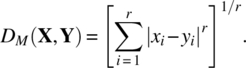
Clustering is a method of grouping a set of elements or a complicated data set into some homogeneous groups. Other than subjective observation, a very nature objective method of clustering is based on a distance and similarity measure. In time domain, given two r‐dimensional observations, X = (x1, x2, …, xr) and Y = (y1, y2, …, yr). Some commonly used distance and similarity measures include the following.
- Euclidian distance:

- Minkowski distance:
- Canberra distance:

- Kullback–Leibler (KL) distance:
Statistically, we see that a good distance and similarity measure is a distribution‐based or a model‐based approach briefly introduced in Section 10.2.3, where an associated probability distribution is used in clustering. In terms of frequency domain spectral density distributions, given two spectra, fi(ωk) and fj(ωk), 0 < ωk < 1/2, the most commonly used similarity measure of spectrum is the KL distance, defined as

and its symmetric form as the quasi‐distance D(fi, fj) = KL(fi, fj) + KL(fj, fi). It turns out that

which is the distance we will use in the frequency domain.
Based on a distance measure, we have hierarchical and nonhierarchical clustering methods.
Given a set of N elements, the hierarchical clustering method includes the following steps:
- Step 1. Begin with N clusters by assuming each of the elements is an individual cluster. The distances between clusters are the same as the distances between elements.
- Step 2. Combine the two elements that are most similar with minimum distance and form a new cluster. This leads to one less cluster.
- Step 3. Compute distances between the newly formed cluster and other remaining clusters.
- Step 4. Repeat steps 2 and 3 a total (N − 1) times so that all become a single cluster after the algorithm terminates, with the results shown in a dendrogram.
It should be noted that step 3 can be done in different ways or algorithms. The first way is “single linkage” in which the minimum distance between each element of newly formed cluster and other clusters is computed. The second way is “complete linkage” in which the maximum distance between each element of newly formed cluster and other clusters is computed. The third way is “average linkage” in which the average distance between each element of newly formed cluster and other clusters is computed. The fourth way is “median linkage” in which the median distance between each element is used as introduced by Tibshirani et al. (2001).
In terms of nonhierarchical methods, the most popular approach is the K‐means method, which assigns each item to the cluster having the nearest centroid (mean) or assigned center point.
In terms of deciding an optimal number of clusters, we will use the total within sum of squares (TWSS), which measures total intra‐cluster variation and we would like it to be as small as possible. We will illustrate its use through an empirical example in the next section.
10.6.2 Forming aggregate data through both time domain and frequency domain clustering
In modeling the U.S. yearly STD data, we created aggregate data based on MMWR regions and four STD regions. We can also form the aggregate groups using clustering as illustrated in the following.
10.6.2.1 Example of time domain clustering
Recall the data set of U.S. yearly STD morbidity rates from 1984 to 2013, which we have analyzed earlier. It contains 43 states plus Washington D.C. So, we have a set of m = 44 elements, each with a length of n = 29. Based on the model‐based clustering method, the 44 elements are classified into three clusters with the detail given in Table 10.11.
Table 10.11 The model‐based clustering of the STD data.
| Cluster | Number of states | States |
| 1 | 16 | CT, NY, DC, PA, FL, GA, MS, IL, MI, OH, WI, AR, LA, MO, CA, WA |
| 2 | 15 | MA, NJ, DE, MD, VA, AL, NC, SC, TN, IN, TX, IA, KS, ID, OR |
| 3 | 13 | ME, NH, RI, WV, KY, MN, NM, OK, NE, CO, UT, AZ, NV |
10.6.2.2 Example of frequency domain clustering
Next, we will show that the clustering of the STD data can also be done through frequency domain spectral matrices. Specifically, we will use the kernel smoothing method discussed in Chapter 9 to obtain the estimates of spectral matrices. We choose the Daniell smoothing window with bandwidth m = 5. The resulting individual spectra for 44 elements are presented in Figure 10.5.

Figure 10.5 The spectra of the STD data for 43 states plus D.C.
10.6.2.2.1 Clustering using similarity measures
Based on the KL distance and its quasi‐distance form, D(fi, fj), we compute TWSS, which measures total intra‐cluster variation. Figure 10.6 is the plot for TWSS across different numbers of clusters from the STD data set. The location of a bend (knee) in the plot is generally considered to be an indicator of the appropriate number of clusters. It shows that five or six clusters seem to be a good choice.

Figure 10.6 Total within sum of squares plot.
10.6.2.2.2 Clustering by subjective observation
The spectrum matrices in Figure 10.5 clearly indicate a group or cluster pattern. Intuitively, the spectrum of each state can be roughly categorized into the following clusters, which are highly consistent with the MMWR regions. Based on the similarity of spectrums, we can group them in the following six clusters given in Table 10.12.
Table 10.12 Clustering by subjective observation.
| Cluster | Number of states | States |
| 1 | 3 | ME, NH, RI These states are in the North East region. |
| 2 | 4 | CT, NJ, NY, PA These states are in the Middle Atlantic region. |
| 3 | 12 | MA, DE, DC, MD, VA, AL, FL, GA, MS, SC, NC, TN Most of these states are in the South Atlantic and East South Central regions. |
| 4 | 14 | IL, IN, KY, MI, MN, OH, WV, WI, KS, MO, IA, TX, LA, AR These states are in the East North Central, Western North Central, and West South Central regions. |
| 5 | 8 | OK, NE, AZ, NM, NV, ID, UT, CO These states are in the West South Central and Mountain regions. |
| 6 | 3 | CA, OR, WA These states are in the Pacific region. |
10.6.2.2.3 Hierarchical clustering
The dendrograms of the four algorithms for the STD data are shown in Figures 10.7–10.10.

Figure 10.7 Single linkage dendrogram for STD spectra.


Figure 10.10 Median linkage dendrogram for STD spectra.
10.6.2.2.4 Nonhierarchical clustering using the K‐means method
The Partitioning Around Medoids (PAM) is a robust version of the K‐means clustering algorithm. It begins with a selection K objects as medoids, and then we minimize the sum of the dissimilarities of the observations to their closest cluster. We apply PAM to the spectrums of STD data set with K = 4, and obtain the following result in Table 10.13 and its cluster plot in Figure 10.11.
Table 10.13 PAM clustering based on STD spectrums with K = 4.
| Cluster | Number of states | States |
| 1 | 17 | CT, NY, DC, PA, AL, FL, GA, MS, TN, IL, MI, OH, AR, LA, MO, CA, WA |
| 2 | 9 | ME, NH, NM, OK, NE, CO, UT, AZ, NV |
| 3 | 13 | MA, RI, DE, VA, WV, KY, NC, SC, IN, MN, WI, TX, IA |
| 4 | 5 | NJ, MD, KS, ID, OR |

Figure 10.11 PAM cluster plot of the STD data set.
It turns out that the clustering patterns found by the model‐based clustering and the PAM method are very similar. Specifically, the cluster 1 of the model‐based clustering method is almost identical to the cluster 1 of PAM; the cluster 2 of the model‐based clustering method corresponds to the clusters 3 and 4 of PAM method; and cluster 3 of the model‐based clustering method is close to the cluster 2 of the PAM method.
For more discussion and examples of clustering, we refer readers to Tibshirani et al. (2001), Johnson and Wichern (2007), and Izenman (2008), among others.
10.6.3 The specification of aggregate matrix and its associated aggregate dimension
Big data and high‐dimensional problems are everywhere in the age of fast computers and the internet. To address this, we propose aggregation as a dimension reduction method. It is very natural and simple to use, and its performance in forecasting is supported by both simulation and empirical examples as a good method for dimension reduction.
The aggregation matrix A and its associated s can occur in many different specifications. Even based on practical considerations, we can specify different forms of A and s. By choosing s = 1, A becomes a row vector, and any m‐dimensional multivariate time series Zt will aggregate to become a univariate time series Yt. Most of the time, the result of aggregation is meaningful. For example, sales data can be specified in terms of regions or kinds (categories). With regard to housing sales of the 3144 US counties, this data can be aggregated into housing sales for each of the 50 states, into the housing sales of the four regions (East, West, North, and South), and further into the total housing sales of the entire country. We can also specify A and s based on data‐driven considerations, which we will leave to our readers to try.
10.6.4 Be aware of other forms of aggregation
It is important to note that aggregation as a tool for high dimension reduction that we have suggested is contemporal aggregation. Other forms of aggregation include temporal aggregation for a flow variable such as industrial production and a systematic sampling for a stock variable such as the price of a given commodity. However, these techniques are not useful for high dimension reduction, in fact, they will aggravate the problem, since temporal aggregation and systematic sampling lead to very serious information loss as shown in Wei (2006, chapter 20). In fact, limitations of temporal aggregation and systematic sampling have been studied by many researchers including Amemiya and Wu (1972), Brewer (1973), Tiao and Wei (1976), Weiss (1984), Stram and Wei (1986), Lütkepohl (1987), Teles and Wei (2000, 2002), Breitung and Swanson (2002), Teles et al. (1999, 2008), Lee and Wei (2017), and many more. An interesting related topic is how to recover the information loss of temporal aggregation and systematic sampling. One can use either temporal disaggregation or bootstrap, which we will not discuss in this book and refer readers to Wei and Stram (1990), Meyer and Kreiss (2015), Kim and Wei (2018), and Tewes (2018), among others.
Before closing this chapter, we want to point out that high dimension is an important issue in multivariate time series analysis. We introduce a simple and useful method to reduce dimension. For more discussion and applications on high‐dimensional problems, we refer readers to Chen and Qin (2010), Huang et al. (2010), Flamm et al. (2013), Cho and Fryzlewicz (2015), Giraud (2015), Hung et al. (2016), Lee et al. (2016), Gao et al. (2017), Huang and Chiang (2017), and Wood et al. (2017), among others.
10.A Appendix: Parameter estimation results of various procedures
The details of parameter estimation results for the two empirical examples in Section 10.5 are given next.
10.A.1 Further details of the macroeconomic time series
Since we used out‐of‐sample, the estimation results shown in this section is based on in‐sample data from quarter 1 of 1959 to Quarter 4 of 2007.
10.A.1.1 VAR(1)
Based on the AIC criteria, the VAR(1) model was fitted to the data. The least square estimation was used and the estimated coefficient matrix is

It appears that the matrix is not sparse and is noisy. We will compare the estimated coefficient matrix with estimates from other regularization methods in following sections.
10.A.1.2 Lasso
The maximum allowed lag order is set to be 4. The estimates of coefficient matrices are


The estimates of those matrices are much sparser compared to the estimates from the VAR, using least squares.
10.A.1.3 Componentwise
The maximum allowed lag order is set to be 4. The estimates of coefficient matrices are


10.A.1.4 Own‐other
The maximum allowed lag order is set to be 4. The estimates of coefficient matrices are


10.A.1.5 Elementwise
The maximum allowed lag order is set to be 4. The estimates of coefficient matrices are


10.A.1.6 The factor model
In this section, we show the equation of forecasting the first component Z1,t, which is GDP252. Based on Bai and Ng (2002), two factors are selected. The first factors F1,t and the second factor F2,t are shown in Figure 10.A.1.

Figure 10.A.1 The two factors used in factor modeling for the first component Z1,t GDP252.
Suppose we want to obtain ℓ − step ahead forecast for the first component, Z1,t, of those time series by using factors Ft. The equation is:
where X1,t is the first lag of Z1,t. The estimated parameters are presented in Table 10.A.1.
Table 10.A.1 The estimated parameters of the factor model for the first component Z1,t, GDP252.
| Estimate | |
|
|
| 0.0005 | −0.0001 | 0.7599 |
10.A.1.7 The model‐based cluster
The maximum number of clusters allowed is set to be 4 and the AR(1) model is fitted for each cluster. The individual time series is assigned to cluster i if its probability of being in cluster i is the highest. Table 10.A.2 presents probabilities of each time series being in specific clusters (first four columns) and the finally assigned cluster for each time series (the last column). Table 10.A.2 shows that no time series is within cluster 4 based on the estimated probability. Moreover, most of “GDPXXX” time series are assigned to cluster 1, most of “CESXXX” time series are in cluster 2, and most of “IPSXXX” time series are in cluster 2 and 3. The models of cluster 1, 2, and 3 can be written as
where the estimated parameters are shown in Table 10.A.3.
Table 10.A.2 Macroeconomic time series with probabilities of series being in four different clusters and the finally assigned cluster for each series.
| Cluster 1 | Cluster 2 | Cluster 3 | Cluster 4 | Cluster Assigned | |
| GDP252 | 0.505 | 0.441 | 0.053 | 0.002 | 1 |
| GDP253 | 0.001 | 0.000 | 0.704 | 0.295 | 3 |
| GDP254 | 0.499 | 0.501 | 0.000 | 0.000 | 2 |
| GDP255 | 0.559 | 0.098 | 0.328 | 0.015 | 1 |
| GDP256 | 0.016 | 0.000 | 0.626 | 0.357 | 3 |
| GDP257 | 0.540 | 0.093 | 0.352 | 0.015 | 1 |
| GDP258 | 0.554 | 0.097 | 0.342 | 0.006 | 1 |
| GDP259 | 0.214 | 0.042 | 0.677 | 0.067 | 3 |
| GDP260 | 0.162 | 0.039 | 0.727 | 0.072 | 3 |
| GDP261 | 0.629 | 0.208 | 0.161 | 0.002 | 1 |
| GDP266 | 0.095 | 0.000 | 0.653 | 0.251 | 3 |
| GDP267 | 0.558 | 0.299 | 0.143 | 0.000 | 1 |
| GDP268 | 0.500 | 0.300 | 0.186 | 0.015 | 1 |
| GDP269 | 0.556 | 0.302 | 0.142 | 0.000 | 1 |
| GDP271 | 0.690 | 0.310 | 0.000 | 0.000 | 1 |
| GDP272 | 0.502 | 0.297 | 0.186 | 0.015 | 1 |
| GDP274 | 0.559 | 0.098 | 0.328 | 0.015 | 1 |
| GDP275 | 0.559 | 0.098 | 0.328 | 0.015 | 1 |
| GDP276 | 0.559 | 0.098 | 0.328 | 0.015 | 1 |
| GDP277 | 0.557 | 0.098 | 0.328 | 0.017 | 1 |
| GDP278 | 0.558 | 0.299 | 0.143 | 0.000 | 1 |
| GDP279 | 0.502 | 0.298 | 0.186 | 0.015 | 1 |
| GDP280 | 0.557 | 0.219 | 0.215 | 0.009 | 1 |
| GDP281 | 0.511 | 0.349 | 0.128 | 0.013 | 1 |
| GDP282 | 0.484 | 0.038 | 0.373 | 0.104 | 1 |
| GDP284 | 0.559 | 0.098 | 0.328 | 0.015 | 1 |
| GDP285 | 0.136 | 0.000 | 0.634 | 0.230 | 3 |
| GDP286 | 0.745 | 0.110 | 0.143 | 0.002 | 1 |
| GDP287 | 0.838 | 0.049 | 0.036 | 0.077 | 1 |
| GDP288 | 0.860 | 0.135 | 0.002 | 0.002 | 1 |
| GDP289 | 0.860 | 0.135 | 0.002 | 0.002 | 1 |
| GDP290 | 0.860 | 0.135 | 0.002 | 0.002 | 1 |
| GDP291 | 0.499 | 0.501 | 0.000 | 0.000 | 2 |
| GDP292 | 0.499 | 0.501 | 0.000 | 0.000 | 2 |
| IPS11 | 0.499 | 0.501 | 0.000 | 0.000 | 2 |
| IPS299 | 0.499 | 0.501 | 0.000 | 0.000 | 2 |
| IPS12 | 0.860 | 0.135 | 0.002 | 0.002 | 1 |
| IPS13 | 0.042 | 0.000 | 0.684 | 0.273 | 3 |
| IPS18 | 0.860 | 0.135 | 0.002 | 0.002 | 1 |
| IPS25 | 0.499 | 0.501 | 0.000 | 0.000 | 1 |
| IPS32 | 0.061 | 0.000 | 0.694 | 0.245 | 3 |
| IPS34 | 0.068 | 0.002 | 0.708 | 0.222 | 3 |
| IPS38 | 0.499 | 0.501 | 0.000 | 0.000 | 2 |
| IPS43 | 0.499 | 0.501 | 0.000 | 0.000 | 2 |
| IPS307 | 0.000 | 0.000 | 0.680 | 0.320 | 3 |
| IPS306 | 0.010 | 0.000 | 0.730 | 0.260 | 3 |
| CES275 | 0.499 | 0.501 | 0.000 | 0.000 | 2 |
| CES277 | 0.499 | 0.501 | 0.000 | 0.000 | 2 |
| CES278 | 0.499 | 0.501 | 0.000 | 0.000 | 2 |
| CES003 | 0.499 | 0.501 | 0.000 | 0.000 | 2 |
| CES006 | 0.196 | 0.016 | 0.627 | 0.161 | 3 |
| CES011 | 0.499 | 0.501 | 0.000 | 0.000 | 2 |
| CES015 | 0.499 | 0.501 | 0.000 | 0.000 | 2 |
| CES017 | 0.499 | 0.501 | 0.000 | 0.000 | 2 |
| CES033 | 0.499 | 0.501 | 0.000 | 0.000 | 2 |
| CES046 | 0.499 | 0.501 | 0.000 | 0.000 | 2 |
| CES048 | 0.499 | 0.501 | 0.000 | 0.000 | 2 |
| CES049 | 0.499 | 0.501 | 0.000 | 0.000 | 2 |
| CES053 | 0.499 | 0.501 | 0.000 | 0.000 | 2 |
| CES088 | 0.499 | 0.501 | 0.000 | 0.000 | 2 |
| CES140 | 0.499 | 0.501 | 0.000 | 0.000 | 2 |
Table 10.A.3 The estimated parameters of the model‐based clustering for the macroeconomic time series.
| Estimates | |
|
|
|
|
|
| 0.398 | 0.033 | 0.541 | 0.032 | 0.155 | 0.039 |
10.A.1.8 The proposed method
The 61 time series are aggregated into trivariate time series, GDP, IPS, and CES. We fit a VAR(p) model,

The best fitted model is p = 2 based on AIC. Estimates of coefficient matrices along with their standard errors (in parenthesis) are shown next:

10.A.2 Further details of the STD time series
10.A.2.1 VAR
Since the number of dimension m = 44 is much greater than the number of observations n = 29, the ordinary least square estimation without any restrictions failed for this model.
10.A.2.2 Lasso


10.A.2.3 Componentwise


10.A.2.4 Own‐other
The maximum allowed lag order is set to be 4.


10.A.2.5 Elementwise
The maximum allowed lag order is set to be 4.


10.A.2.6 The STAR model
Since the STD data are collected from different states, which are spatially related, the space–time modeling can be used. Based on AIC criteria, the STAR(22, 1) model is used and can be written as

The estimates are presented in Table 10.A.4.
Table 10.A.4 Estimated parameters for the STAR model.
| Estimates | |
|
|
|
|
| 0.074 | 0.286 | 0.239 | −0.126 | 0.065 |
Moreover, the weighting matrices, W(0), W(1), and W(2), are specified by using spatial relationship between states and are shown next:


10.A.2.7 The factor model
In this section, we show the equation for forecasting the first component Z1,t, which is the STD rate in Connecticut. Six factors are selected, and the estimated factor scores are shown in Figure 10.A.2.

Figure 10.A.2 The plot of estimated six common factor scores for the STD data set.
To compute the ℓ − step ahead forecast for the first component, Z1,t + ℓ, we will use the following model equation, which is:
where X1,t is the first lag of Z1,t. The estimated parameters are presented in Table 10.A.5.
Table 10.A.5 The estimated parameters of the factor model for the first component, STD rate in Connecticut.
| Estimate | |
|
|
|
|
|
|
| 0.054 | 0.232 | −0.056 | −0.100 | −0.208 | −0.203 | 0.234 |
10.A.2.8 The model‐based cluster
The maximum number of clusters allowed is set to be 4 and the AR(1) model is fitted for each cluster. Each time series is assigned to cluster i if its probability of being in cluster i is the highest. Probabilities of each time series being in specific clusters (first four columns) and the finally assigned cluster for each time series (the last column) are presented in Table 10.A.6. It shows that no time series was assigned to cluster 1. The models of cluster 1, 2, 3, and 4 can be written as
where the estimated parameters are shown in Table 10.A.7.
Table 10.A.6 STD time series with probabilities of the series being in four different clusters and the finally assigned cluster for each series.
| Cluster 1 | Cluster 2 | Cluster 3 | Cluster 4 | Assigned Cluster | |
| CT | 0.02 | 0.62 | 0.00 | 0.36 | 2 |
| ME | 0.05 | 0.00 | 0.94 | 0.01 | 3 |
| MA | 0.23 | 0.12 | 0.14 | 0.51 | 4 |
| NH | 0.10 | 0.00 | 0.85 | 0.05 | 3 |
| RI | 0.13 | 0.00 | 0.83 | 0.04 | 3 |
| NJ | 0.10 | 0.36 | 0.01 | 0.53 | 4 |
| NY | 0.02 | 0.66 | 0.00 | 0.32 | 2 |
| DE | 0.21 | 0.16 | 0.08 | 0.55 | 4 |
| DC | 0.02 | 0.61 | 0.00 | 0.36 | 2 |
| MD | 0.18 | 0.22 | 0.03 | 0.57 | 4 |
| PA | 0.02 | 0.63 | 0.00 | 0.35 | 2 |
| VA | 0.23 | 0.12 | 0.13 | 0.52 | 4 |
| WV | 0.04 | 0.00 | 0.96 | 0.00 | 3 |
| AL | 0.07 | 0.42 | 0.00 | 0.50 | 4 |
| FL | 0.01 | 0.70 | 0.00 | 0.29 | 2 |
| GA | 0.01 | 0.68 | 0.00 | 0.31 | 2 |
| KY | 0.23 | 0.03 | 0.48 | 0.26 | 3 |
| MS | 0.03 | 0.55 | 0.00 | 0.42 | 2 |
| NC | 0.07 | 0.43 | 0.00 | 0.49 | 4 |
| SC | 0.17 | 0.23 | 0.03 | 0.57 | 4 |
| TN | 0.11 | 0.34 | 0.01 | 0.54 | 4 |
| IL | 0.03 | 0.56 | 0.00 | 0.40 | 2 |
| IN | 0.19 | 0.19 | 0.06 | 0.56 | 4 |
| MI | 0.03 | 0.59 | 0.00 | 0.38 | 2 |
| MN | 0.13 | 0.22 | 0.34 | 0.31 | 3 |
| OH | 0.01 | 0.76 | 0.00 | 0.23 | 2 |
| WI | 0.07 | 0.43 | 0.00 | 0.50 | 4 |
| AR | 0.03 | 0.56 | 0.00 | 0.41 | 2 |
| LA | 0.01 | 0.74 | 0.00 | 0.26 | 2 |
| NM | 0.04 | 0.00 | 0.96 | 0.00 | 3 |
| OK | 0.07 | 0.00 | 0.92 | 0.01 | 3 |
| TX | 0.12 | 0.31 | 0.01 | 0.55 | 4 |
| IA | 0.17 | 0.22 | 0.14 | 0.47 | 4 |
| KS | 0.18 | 0.20 | 0.06 | 0.56 | 4 |
| MO | 0.02 | 0.64 | 0.00 | 0.34 | 2 |
| NE | 0.06 | 0.00 | 0.92 | 0.02 | 3 |
| CO | 0.16 | 0.02 | 0.68 | 0.15 | 3 |
| UT | 0.12 | 0.01 | 0.78 | 0.09 | 3 |
| AZ | 0.07 | 0.00 | 0.92 | 0.01 | 3 |
| CA | 0.05 | 0.49 | 0.00 | 0.45 | 2 |
| NV | 0.04 | 0.00 | 0.95 | 0.00 | 3 |
| ID | 0.24 | 0.09 | 0.22 | 0.45 | 4 |
| OR | 0.17 | 0.23 | 0.04 | 0.56 | 4 |
| WA | 0.02 | 0.68 | 0.00 | 0.31 | 2 |
Table 10.A.7 The estimated parameters of the model‐based clustering for the STD data set.
| Estimates | |
|
|
|
|
|
|
|
| 0.121 | 1.032 | 0.518 | 0.929 | −0.246 | 0.989 | 0.349 | 0.999 |
10.A.2.9 The proposed method
The 44 time series are aggregated into MMWR region (9 time series) and fit a VAR(p) model, such that

The best fitted model is p = 1 based AIC. The estimate of the coefficient matrix and the associated standard error (in parenthesis) are shown next.

If we aggregate the 44 time series into STD region (4 time series) and fit a VAR(p) model, the best fitted model is p = 4 with the following estimates of the associated coefficient matrices.

Projects
- Find a high‐dimensional time series data set in a social science field, perform its principal component and factor analyses, and complete your analysis with a written report and attached software code.
- Use the aggregation method to build an aggregate model for the data set from Project 1 and complete your analysis with a written report and attached software code.
- Perform your analyses in Projects 1 and 2 with (n − 5) observations, then compare the results in terms of their next five‐step forecasts.
- Find a high‐dimensional time series data set in a natural science‐related field, and perform its analysis with a written report and associated software code.
- Find a real high‐dimensional vector time series data set of your interest, use various dimension reduction methods to analyze your data set, make comparisons, and complete your analysis with a written report and associated software code.
References
- Amemiya, T. and Wu, R.Y. (1972). The effect of aggregation on prediction in the autoregressive model. Journal of American Statistical Association 339: 628–632.
- Bai, J. and Ng, S. (2002). Determining the number of factors in approximate factor models. Econometrica 70: 191–221.
- Banfield, J. and Raftery, A. (1993). Model‐based cluster Gaussian and non‐Gaussian clustering. Biometrics 49: 803–821.
- Box, G.E.P., Jenkins, G.M., Reinsel, G.C., and Ljung, G.M. (2015). Time Series Analysis, Forecasting and Control, 5e. Wiley.
- Box, G.E.P. and Tiao, G.C. (1977). A canonical analysis of multiple times series. Biometrika 64: 355–370.
- Breitung, J. and Swanson, N.R. (2002). Temporal aggregation and spurious instantaneous causality in multiple time series models. Journal of Time Series Analysis 23: 651–666.
- Brewer, K.R.W. (1973). Some consequences of temporal aggregation and systematic sampling for ARMA and ARMAX models. Journal of Econometrics 1: 133–154.
- Cattell, R.B. (1943). The description of personality: basic traits resolved into clusters. Journal of Abnormal and Social Psychology 38: 476–506.
- Chen, S.X. and Qin, Y.L. (2010). A two‐sample test for high‐dimensional data with applications to gene‐set testing. The Annals of Statistics 38: 808–835.
- Cho, H. and Fryzlewicz, P. (2015). Multiple‐change‐point detection for high dimensional time series via sparsified binary segmentation. Journal of the Royal Statistical Society, Series B 77: 475–507.
- Cliff, A.D. and Ord, J. (1975). Model building and the analysis of spatial pattern in human geography. Journal of the Royal Statistical Society, Series B 37: 297–348.
- Flamm, C., Graef, A., Pirker, S., Baumgartner, C. and Deistler, M. (2013). Influence analysis for high‐dimensional time series with an application to epileptic seizure onset zone detection. Journal of Neuroscience Methods 214: 80–90.
- Fraley, C. and Raftery, A. (2002). Model‐based cluster clustering, discriminant analysis, and density estimation. Journal of the American Statistical Association 97: 458–470.
- Gao, J., Han, X., Pan, G., and Yang, Y. (2017). High dimensional correlation matrices: the central limit theorem and its applications. Journal of Royal Statistical Society, Series B 79: 677–693.
- Gehman, A. (2016). The Effects of Spatial Aggregation on Spatial Time Series Modeling and Forecasting, PhD dissertation, Temple University.
- Giraud, C. (2015). Introduction to High‐Dimensional Statistics. Chapman and Hall/CRC.
- Hamilton, J.D. (1994). Time Series Analysis. Princeton University Press.
- Hannon, E.J. (1970). Multiple Time Series. Wiley.
- Hsu, N., Hung, H., and Chang, Y. (2008). Subset selection for vector autoregressive processes using lasso. Computational Statistics and Data Analysis 52: 3645–3657.
- Huang, M.Y. and Chiang, C.T. (2017). An efficient semiparametric estimation approach for the sufficient dimension reduction model. Journal of American Statistical Association 112: 1296–1310.
- Huang, H.C., Hsu, N.J., Theobald, D.M., and Breidt, F.J. (2010). Spatial lasso with applications to GIS model selection. Journal of Computational and Graphical Statistics 19 (4): 963–983.
- Hung, H., Liu, C.Y., and Lu, H.H.S. (2016). Sufficient dimension reduction with additional information. Biostatistics 17: 405–421.
- Izenman, A.J. (2008). Modern Multivariate Statistical Techniques. Springer.
- Johnson, R.A. and Wichern, D.W. (2007). Applied Multivariate Statistical Analysis, 6e. Pearson Prentice Hall.
- Kalman, R.E. (1960). A new approach to linear filtering and prediction problems. Transactions of the ASME – Journal of Basic Engineering, Series D 82: 35–45.
- Kim, H.C., and Wei, W.W.S. (2018). Block bootstrap and effect of aggregation and systematic sampling. A research manuscript.
- Kohn, R. (1982). When is an aggregate of a time series efficiently forecast by its past? Journal of Econometrics 18: 337–349.
- Koop, G.M. (2013). Forecasting with medium and large Bayesian VARs. Journal of Applied Econometrics 28: 177–203.
- Lee, B.H. and Wei, W.W.S. (2017). The use of temporally aggregation data on detecting a mean change of a time series process. Communications in Statistics‐Theory and Methods 46 (12): 5851–5871.
- Lee, N., Choi, H., and Kim, S.H. (2016). Bayes shrinkage estimation for high‐dimensional VAR models with scale mixture of normal distributions for noise. Computational Statistics and Data Analysis 101: 250–276.
- Li, Z., and Wei, W.W.S. (2017). The use of contemporal aggregation for high‐dimensional time Series. A research manuscript.
- Lütkepohl, H. (1984). Forecasting contemporaneously aggregated vector ARMA processes. Journal of Business and Economic Statistics 2: 201–214.
- Lütkepohl, H. (1987). Forecasting Aggregated Vector ARMA Processes. Springer.
- Lütkepohl, H. (2007). New Introduction to Multiple Time Series Analysis. Springer.
- MacQueen, J. (1967). Some methods for classification and analysis of multivariate observations. In: Proceedings of the 5th Berkeley Symposium on Mathematical Statistics and Probability, vol. 1 (ed. L.M. Cam and J. Neyman), 281–297. University of California Press.
- Matteson, D.S. and Tsay, R.S. (2011). Dynamic orthogonal components for multivariate time series. Journal of the American Statistical Association 106: 1450–1463.
- McLachlan, G. and Basford, K.E. (1988). Mixture Models: Inference and Applications to Clustering. Marcel Dekker.
- Meyer, M. and Kreiss, J. (2015). On the vector autoregressive sieve bootstrap. Journal of Time Series Analysis 36: 377–397.
- Nicholson, W.B., Bien, J., and Matteson, D.S. (2016). High dimensional forecasting via interpretable vector autoregression, arXiv: 1412.525v2.
- Pfeifer, P.E. and Deutsch, S.J. (1980a). A three‐stage iterative procedure for space‐time modeling. Technometrics 22 (1): 35–47.
- Pfeifer, P.E. and Deutsch, S.J. (1980b). Identification and interpretation of the first order space‐time ARMA models. Technometrics 22: 397–408.
- Pfeifer, P.E. and Deutsch, S.J. (1980c). Stationary and inevitability regions for low order STARMA models. Communications in Statistics Part B: Simulation and Computation 9: 551–562.
- Reinsel, G.C. (1997). Elements of Multivariate Time Series Analysis, 2e. Springer‐Verlag.
- Rose, D. (1977). Forecasting aggregates of independent ARIMA process. Journal of Econometrics 5: 323–345.
- Scrucca, L. (2010). Dimension reduction for model‐based cluster clustering. Statistics and Computing 20 (4): 471–484.
- Song, S., and Bickel, P. (2011). Large vector autoregressions, arXiv: 1106.3915.
- Stock, J.H. and Watson, M.W. (2002a). Forecasting using principal components from a large number of predictors. Journal of the American Statistical Association 97: 1167–1179.
- Stock, J.H. and Watson, M.W. (2002b). Macroeconomic forecasting using diffusion index. Journal of Business and Economics Statistics 20: 1147–1162.
- Stock, J.H. and Watson, M.W. (2009). Forecasting in dynamic factor models subject to structural instability. In: The Methodology and Practice of Econometrics (ed. N. Shephard and J. Castle), 173–206. Oxford: Oxford University Press.
- Stram, D.O. and Wei, W.W.S. (1986). Temporal aggregation in the ARIMA process. Journal of Time Series Analysis 7 (4): 279–292.
- Teles, P., Hodgess, E., and Wei, W.W.S. (2008). Testing a unit root based on aggregate time series. Communications in Statistics – Theory and Methods 37: 565–590.
- Teles, P. and Wei, W.W.S. (2000). The effects of temporal aggregation on tests of linearity of a time series. Computational Statistics and Data Analysis 34: 91–103.
- Teles, P. and Wei, W.W.S. (2002). The use of aggregate time series in testing for Gaussianity. Journal of Time Series Analysis 23: 95–116.
- Teles, P., Wei, W.W.S., and Crato, N. (1999). The use of aggregate time series in testing for long memory. Bulletin of International Statistical Institute 3: 341–342.
- Tewes, J. (2018). Block bootstrap for the empirical process of long‐range dependent data. Journal of Time Series Analysis 39: 28–53.
- Tiao, G.C. and Guttman, I. (1980). Forecasting contemporal aggregate of multiple time series. Journal of Econometrics 12: 219–230.
- Tiao, G.C. and Wei, W.W.S. (1976). Effect of temporal aggregation on the dynamic relationship of two time series variables. Biometrika 63: 513–523.
- Tibshirani, R. (1996). Regression shrinkage and selection via the lasso. Journal of Royal Statistical Society, Series B 58: 267–288.
- Tibshirani, R., Walther, G., and Hastie, T. (2001). Estimating the number of clusters in a data set via the gap statistics. Journal of Royal Statistical Association, Series B 63: 411–423.
- Tryon, R.C. (1939). Cluster Analysis: Correlation Profile and Orthometric (Factor) Analysis for the Isolation of Unities in Mind and Personality. Edwards Brothers.
- Tsay, R.S. (2013). Multivariate Time Series Analysis with R and Financial Applications. Wiley.
- Wang, S. and Zhou, J. (2008). Variable selection for model‐based high‐dimensional clustering and its application to microarray data. Biometrics 64: 440–448.
- Wang, Y., Tsay, R.S., Ledolter, J., and Shrestha, K.M. (2013). Forecasting simultaneously high‐dimensional time series: a robust model‐based clustering approach. Journal of Forecasting 32: 673–684.
- Ward, J.H. (1963). Hierarchical grouping to optimize an objective function. Journal of the American Statistical Association 58: 234–244.
- Wei, W.W.S. (2006). Time Series Analysis – Univariate and Multivariate Methods, 2e. Boston: Pearson Addison‐Wesley.
- Wei, W.W.S. and Abraham, B. (1981). Forecasting contemporal time series aggregates. Communications in Statistics – Theory and Methods 10: 1335–1344.
- Wei, W.W.S. and Stram, D.D.O. (1990). Disaggregation of time series models. Journal of Royal Statistical Society, Series B 52: 453–467.
- Wei, W.W.S. (2018). Dimension reduction in high dimensional multivariate time series analysis. To appear in Contemporary Biostatistics with Biopharmaceutical Application, ICSA Book Series in Statistics.
- Weiss, A.A. (1984). Systematic sampling and temporal aggregation in time series models. Journal of Econometrics 26: 255–278.
- Wood, S.N., Li, Z., Shaddick, G., and Augustin, N.H. (2017). Generalized additive models for gigadata: modeling the U.K. black smoke network daily data. Journal of the American Statistical Association 112: 1199–1210.
- Yuan, M. and Lin, Y. (2006). Model selection and estimation in regression with grouped variables. Journal of the Royal Statistical Society, Series B 68: 49–67.