Search in book...
Toggle Font Controls
Create new playlist

Name your new playlist

Playlist description (optional)
Sign In

Email address

Password

Forgot Password?

or

Continue with Facebook

Continue with Google
Sign Up

Full Name

Email address

Confirm Email Address

Password

or

Continue with Facebook

Continue with Google

8
Space–time series models

As indicated in Chapter 1, although the ordering of a time series is usually through time, it may also be ordered through space. If distances of spaces between observations are equal, the time series models and methods discussed earlier are equally applicable. However, in practice, we often see the phenomenon where regular time series are observed in different regions, and the point of interest is the study of the spatial patterns of these series. For example, in studying a traffic pattern of a certain location, traffic flow data is collected at constant intervals of time not only at that location but also at neighboring locations. In studying the prices of a certain commodity in a city, we not only want to study the price series of that commodity in that city but also the prices of the same commodity in nearby cities. In this chapter, we will present methods and models that can be used to describe spatial time series that are related to both time and space.

8.1 Introduction

One way to model the space–time series is to treat them as a vector time series where the ith component corresponds to the ith location. Thus,

(8.1)

One can use the methods that were introduced in Chapter 2 to construct a vector autoregressive moving average VARMA(p,q) model or a vector autoregressive VAR(p) model for the series and use it to forecast and make inferences.

Alternatively, by classifying the spaces (locations) into different groups (regions), these spatial series are often measurements of the same phenomenon from several locations. For example, in studying the prices of a certain commodity in a city, we may divide the city into different regions where each region includes certain city blocks and the measurements are prices of the commodity under study. Hence, we can treat the spatial series at different locations in these groups (regions) at time t as repeated measurements at time t.

More specifically, we can present the spatial series for time from 1 to n as (n × 1) vector time series Z_i,j, where i refers to the ith group (region), and j refers to the jth location. If the purpose of the study is to find out whether there are any differences between groups (regions), we can use the methods discussed in the repeated measurements in Chapter 7 to analyze the data set, where locations in each group (region) constitute a random sample.

In this chapter, we will introduce another modeling method specifically designed for space–time series and illustrate the method with detailed examples.

8.2 Space–time autoregressive integrated moving average (STARIMA) models

In this section, we will discuss an approach where we build a model that deals not only the serial dependence but also spatial dependence between observations at each time point. Specifically, we will introduce a class of time series models where the structure of spatial dependence is incorporated into the commonly used ARIMA(p,d,q) models, which are found to be useful in many applications.

8.2.1 Spatial weighting matrix

To study space and time dependence, first we need to specify the order of spatial neighbors that reflects their distances to a particular location. Conventionally, the first order neighbors are closer than the second order ones, and the second order neighbors are closer than the third order neighbors, and so on. A standard definition of spatial order is sometimes available, but other times a model builder may need to define these orders so that they are suitable to the particular application.

Suppose that there are a total of m locations and we let Z_t = [Z_1,t, Z_2,t, … , Z_m,t]^′ be the vector of times series of these m locations. Based on the spatial orders, with respect to the time series at location i, we will assign weights related to this location, such that its value is nonzero only when the location j is the ℓ^th order neighbors of i, and the sum of these weights is equal to 1. In other words, with respect to location i, we have where

Combining these weights, for all m locations, we have the spatial weight matrix for the neighborhood, which is a m × m matrix with being nonzero if and only if locations i and j are in the same ℓ^th order neighbor and each row sums to 1. The weight can be chosen to reflect physical properties such as border length or distance of neighboring locations. One can also assign equal weights to all the locations of the same spatial order. Clearly, W⁽⁰⁾ = I, an identity matrix, because each location is its own zero^th order neighbor.

If we define the first order neighborhoods of a region to be those sharing a border with it, the second order neighborhoods of a region to be those sharing a border with the first order neighborhoods, and the third order neighborhoods of a region to be those sharing a border with the second order neighborhoods, then for the northeast states of USA given in Figure 8.1, we will have Table 8.1 of the three‐order neighborhoods.

Table 8.1 Spatial neighborhoods of 11 states in the Northeast United States.

Region (m)	First Order Neighborhood	Second Order Neighborhood	Third Order Neighborhood
CT(1)	MA, NY, RI	NH, NJ, PA, VT	DE, MD, ME
DE(2)	MD, NJ, PA	NY	CT, MA, VT
MA(3)	CT, NH, NY, RI, VT	ME, NJ, PA	DE, MD
MD(4)	DE, PA	NJ, NY	CT, MA, VT
ME(5)	NH	MA, VT	CT, NY, RI
NH(6)	MA, ME, VT	CT, NY, RI	NJ, PA
NJ(7)	DE, NY, PA	CT, MA, MD, VT	NH, RI
NY(8)	CT, MA, NJ, PA, VT	DE, MD, NH, RI	ME
PA(9)	DE, MD, NJ, NY	CT, MA, VT	NH, RI
RI(10)	CT, MA	NH, NY, VT	ME, NJ, PA
VT(11)	MA, NH, NY	CT, ME, NJ, PA, RI,	DE, MD

If we assign equal weight to all the locations of the same spatial order, the weighting matrix of W⁽¹⁾ will be

(8.2a)

Similarly, we have

(8.2b)

and

(8.2c)

⊲

8.2.2 STARIMA models

Thus, incorporating the structure of spatial dependence into a vector VARIMA model, we have the following space–time autoregressive integrated moving average (STARIMA) model,

(8.3)

where

a_t is a Gaussian vector white noise process with zero‐mean vector 0, and covariance matrix structure

(8.4)

and Σ is a m × m symmetric positive definite matrix. D(B) is a proper differencing operator defined similarly as in Eq. (2.59) of Chapter 2. In this application, since component series are observations of the same nature in different locations, the differencing operator could simply be D(B) = (1 − B)^dI. ϕ_k,ℓ and θ_k,ℓ are autoregressive and moving average parameters at time lag k and space lag ℓ. respectively. p is the autoregressive order, q is the moving average order, a_k is the spatial order for the k^th autoregressive term, and m_k is the spatial order for the k^th moving average term.

It should be noted that the variance of each time series Z_i,t is assumed to be constant. If not, a suitable variance stabilization transformation is assumed to be used to obtain Z_i,t. For simplicity, we will simply denote the model as a model.

The STARIMA model in Eq. (8.3) can be extended to a seasonal STARIMA model that contains both seasonal and non‐seasonal AR and MA polynomials as follows,

(8.5)

where

D(B^s) = (1 − B^s)^DI, and s is a seasonal period. α_k,ℓ and β_k,ℓ are seasonal autoregressive and seasonal moving average parameters at time lag k and space lag ℓ, respectively. P is the seasonal autoregressive order, Q is the seasonal moving average order, λ_k is the spatial order for the k^th seasonal autoregressive term, and τ_k is the spatial order for the k^th seasonal moving average term. For simplicity, we will denote the seasonal STARIMA model with a seasonal period s in Eq. (8.5) as

8.2.3 STARMA models

For a zero‐mean stationary spatial time series, the model in Eq. (8.3) reduces to the following space–time autoregressive moving average model,

(8.6)

where the zeros of lie outside the unit circle.

The model becomes a space–time autoregressive () model when q = 0. It becomes a space–time moving average () model when p = 0. The STAR models were first introduced by Cliff and Ord (1975a, 1975b), and Martin and Oeppen (1975), and further extended to STARMA models by Pfeifer and Deutsch (1980a, b, c).

Since a stationary model can be approximated by an autoregressive model, because of its easier interpretation, the most widely used STARMA models in practice are models,

(8.7)

where Z_t is a zero‐mean stationary spatial time series or a proper transformed and differenced series of a nonstationary spatial time series.

8.2.4 ST‐ACF and ST‐PACF

Similar to the vector time series models, the important characteristics of STARMA models are shown through their space–time autocorrelation function (ST‐ACF) and space–time partial autocorrelation function (ST‐PACF).

Without loss of generality, we will assume a zero‐mean spatial time series. To properly incorporate the space weighting matrices in the analysis, the ST‐ACF for ℓ^th neighbors at time lag k is given by

(8.11)

where the space–time autocovariance function between i^th and j^th neighbors at time lag k for the m‐dimensional space–time process is defined by:

(8.12)

The sample ST‐ACF, is thus given by

(8.13)

Similar to the ARMA models, we can use space–time analog of the Yule–Walker equations to derive the ST‐PACF. Specifically, in Eq. (8.7), we replace a₁, …, and a_p by λ = max(a₁, …, a_p). In other words, we consider the following STAR(p_{λ,…, λ}) model

(8.14)

Pre‐multiplying both sides of Eq. (8.14) by [W^(h)Z_t − s]^′ and taking expectation, we have the space–time analog of the Yule–Walker equations,

(8.15)

The ST‐PACF is obtained as the last coefficient, ϕ_p,ℓ, for ℓ = 0, 1, …, λ, from the solution of the successively solving the system of equations for each p = 1, 2, …, s = p, each set of ℓ = {0}, {0, 1}, …, {0, 1, …λ}, and h = {0}, {0, 1}, …, {0, 1, …λ}.

As an illustration, let us first consider the computation of some specific STAR models.

Example 8.4

Now let us consider the ST‐PACF of the STAR(2_{3, 2}) model. In this case, p = 2, and λ = 3, and ℓ = 0, 1, 2, 3. The solution of the successive systems of equations becomes:

p = 1, s = 1, ℓ = 0, h = 0, and hence

which will lead to ϕ_1,0;
p = 1, s = 1, ℓ = 0, 1, h = 0, 1, and hence

which will lead to ϕ_1,1;
p = 1, s = 1, ℓ = 0, 1, 2, h = 0, 1, 2, and hence

which will lead to ϕ_1,2;
p = 1, s = 1, ℓ = 0, 1, 2, 3, h = 0, 1, 2, 3, and hence

which will lead to ϕ_1,3.
p = 2, s = 2, ℓ = 0, h = 0, and hence

Since ϕ_1,0 is known from (1), this leads to ϕ_2,0;
p = 2, s = 2, ℓ = 0, 1, h = 0, 1, and hence

Since ϕ_1,0 and ϕ_1,1 are known from (1) and (2), this leads to ϕ_2,1;
p = 2, s = 2, ℓ = 0, 1, 2, h = 0, 1, 2, and hence

Since ϕ_{1, 0}, ϕ_{1, 1} and ϕ_{1, 2} are known from (1), (2), and (3), this leads to ϕ_2,2. For the STAR(2_3,2) model, we have ϕ_1,0, ϕ_1,1, ϕ_1,2, ϕ_1,3, with ϕ_1,j = 0, for j > 3, and ϕ_2,0, ϕ_2,1, ϕ_2,2, with ϕ_2, j = 0, for j > 2.

The sample ST‐PACF is the solution when the sample space–time autocovariances, are used in Eq. (8.15). Following Wei (2006, p. 403), this sample ST‐PACF can also be obtained from the last estimate by successively fitting the model in Eq. (8.7) for p = 1, 2, …, when ℓ varies from 0, 1, … to a, where a is the maximum spatial order to be considered.

In practice, λ and a are normally unknown, and their values are chosen based on a model builder's decision. However, in most cases, the maximum space order is normally no more than 4. For further references, we refer readers to Pfeifer and Deutsch (1980a).

Since these functions involve both time and space, to make the identification easier, we will consider the following two‐way tables and graphs for the sample SP‐ACF and SP‐PACF.

Sample ST‐ACF Table

Time lag/Space Lag	0	1	2	3	…
1					…
2					…
3					…
4					…
.	.	.	.	.	.
.	.	.	.	.	.

Sample ST‐ACF Graph

Graphs of ST-ACF vs. time lag for ST-ACF spatial lag 0 (left) and ST-ACF spatial lag 1 (right), displaying descending–ascending–descending bars with positive and negative values.

Sample ST‐PACF Table

Time lag/Space Lag	0	1	2	3	…
1					…
2					…
3					…
4					…
.	.	.	.	.	.
.	.	.	.	.	.

Sample ST‐PACF Graph

Graphs for ST–PACF spatial lag 0 (left) and lag 1 (right), displaying descending–ascending–descending bars with positive and negative values.

Under the assumption that the a_t are i.i.d. random vectors with E(a_t) = 0 and variance–covariance matrix σ²I, the variance of the sample ST‐ACF and ST‐PACF can be approximated by

(8.16)

and

(8.17)

where m is the number of locations and n is the length of the time series in each location.

8.3 Generalized space–time autoregressive integrated moving average (GSTARIMA) models

It should be pointed out that the parameters ϕ_k,ℓ and θ_k,ℓ in the STARMA or STARIMA models discussed in Section 8.2 are all scalar, which is the same for all locations. To remove this undesirable restriction, the generalized STAR models, denoted by GSTAR models, were first introduced by Borovkova, Lopuhaa, and Ruchjana (2002), and later extended to the following generalized STARMA, denoted by GSTARMA models, by Di Giacinto (2006),

(8.18)

where the assumption of a_t is the same as Eq. (8.3). However, the time lag k and space lag ℓ parameters, Φ_k,ℓ and Θ_k,ℓ, are diagonal matrices instead of scalars. These parameters can vary depending on locations and hence offer more flexibility.

More generally, the model in Eq. (8.18) can be extended to generalized models,

(8.19)

where

and

To include a seasonal phenomenon, we can also extend the seasonal model in Eq. (8.5) to the following generalized seasonal model,

(8.20)

where

and

The coefficients, α_k,ℓ and β_k,ℓ, are (m × m) diagonal matrices of parameters at time lag k and space lag ℓ.

8.4 Iterative model building of STARMA and GSTARMA models

As shown in Example 8.2, a STAR(1₁) model in Eq. (8.8) is equivalent to a first order vector autoregressive VAR(1) model in Eq. (8.10), that is

Thus, one can treat STARMA models as special cases of the vector VARMA models, where the diagonal elements of the m × m autoregressive and moving average parameter matrices are assumed to be equal because the m series represent a single process operating at different locations and the off‐diagonal elements are assumed to be a linear combination of the W^(ℓ) weighting matrices. Obviously, GSTARMA models are also special cases of vector VARMA models.

Similar to the vector VARMA models, STARMA and GSTARMA models are characterized by the ST‐ACF and ST‐PACF. For a STAR or a GSTAR model, its ST‐PACF cuts off after certain temporal and space lags. Similarly, for a STMA or a GSTMA model, its ST‐ACF cuts off after certain temporal and space lags. If neither of these ST‐ACF and ST‐PACF cuts off over time and space, it will be a STARMA or a GSTARMA model.

Once a STARMA model is identified, the parameters are estimated by minimizing

(8.21)

using various nonlinear optimization techniques, which is equivalent to maximize the likelihood function of

(8.22)

discussed in Chapter 2. The insignificant parameters should be removed and a simpler model be re‐estimated until all parameters are statistically significant.

Before a model can be used for forecasting and making inferences, a diagnostic check must be carefully done to make sure that the residuals are approximately white noise. Specifically, we can calculate the residual sample ST‐ACF and ST‐PACF and compare with their estimated standard deviation. If they are not white noise, based on the results of the residual analysis, we need to re‐identify a new model, re‐estimate the parameters, and perform a diagnostic check, which constitutes an iterative process.

8.5 Empirical examples

8.5.1 Vehicular theft data

Example 8.5

From January 2006 through December 2014, over 750,000 crimes were reported among the 21 police districts in Philadelphia, Pennsylvania, shown on the map in Figure 8.3. The most common crimes reported were thefts and burglaries. The total crime followed a seasonal pattern with more crimes in the summer than in the winter.

Figure 8.3 The map of 21 police districts of Philadelphia, PA, USA.

For this analysis, we consider the monthly total of vehicle thefts recorded at the 21 police districts in Philadelphia from January 2006 to December 2014. The data set consists of m = 21 dimensions corresponding to the 21 police districts and is listed as WW8a in the Data Appendix. The monthly total of vehicle thefts from January 2006 to April 2014 was used for model fitting with a total of n = 100 observations. The monthly total of the thefts from May 2014 to December 2014 was held out for the forecast comparison. Figure 8.4 displays these raw counts for the in‐sample time points.

Figure 8.4 Raw vehicle theft counts from 21 police districts in Philadelphia.

Visually, each time series shows a constant mean but varies among districts. For the variance, we compare several values for the Box‐Cox transformation, and λ = 0.5 is chosen for most locations to stabilize the variance. Thus, the square root of each series was performed. Neither regular nor seasonal differencing was required for any of the 21 series. After being square‐root‐transformed and mean centered, the resulting 21 series for t = 1, 2, …, 100, is given in Figure 8.5.

Figure 8.5 The square‐root‐transformed, mean‐centered vehicle theft counts from 21 police districts in Philadelphia.

Bordering districts are defined as first neighbors, and the weighting matrix for W⁽¹⁾ is given in Table 8.2. Models involving additional spatial lags were considered but the parameter estimates were not significant different from 0, and hence the weighting matrices W^(ℓ) for ℓ > 1 are not given.

The patterns in Figure 8.6 show that the sample ST‐ACFs exponentially decay at both regular time lags, seasonal time lags of multiple of 12, and that ST‐PACFs are significant only at time lags 2, 12, and 24, and spatial lag at 1. For a monthly series of seasonal period of 12, we tentatively choose a STAR(2_1,1) × (2_1,1)₁₂ as its possible underlying model. The estimation result is given as follows:

(8.23)

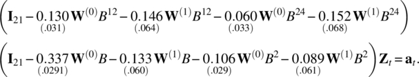
4 Graphs for ST-ACF spatial lag 0 (top left) and lag 1 (top right) and ST-PACF spatial lag 0 (bottom left) and lag 1 (bottom right), displaying bars with positive and negative values. — **Figure 8.6** The sample ST‐ACFs and ST‐PACFs of the data Z_t.

Since the estimate of ϕ_2,1 is only 1.46 standard errors away from 0, we re‐fit a STAR(2_1,0) × (2_1,1)₁₂ model with the following result,

(8.24)

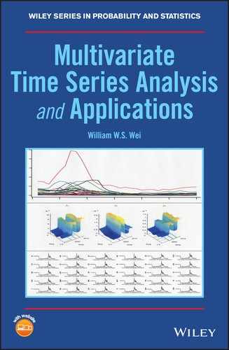
Now, the estimate of α_2,0 is insignificant, so we reduce it to the following STAR(2_1,0) × (2_0,1)₁₂ model,

(8.25)

Now all estimates are significant. In addition, the white noise pattern of the ST‐ACFs and ST‐PACFs of residuals from the fitted model shown in Figure 8.7 indicates that the model is adequate.

4 Graphs illustrating the sample ST-ACFs and ST-PACFs of the residuals from the fitted STAR (21,0) × (20,1)12 model, with short vertical bars with positive and negative values. — **Figure 8.7** The sample ST‐ACFs and ST‐PACFs of the residuals from the fitted STAR(2_1,0) × (2_0,1)₁₂ model.

8.5.2 The annual U.S. labor force count

Example 8.6

The United States Department of Labor provides dozens of variables through the Bureau of Labor Statistics (BLS), many of which could be fitted with various STARMA models. We select non‐seasonally adjusted labor force count for the 48 contiguous states and Washington D.C., for a total of m = 49 locations. The data are annual from 1976 through 2014. This constitutes our raw data, which is listed as WW8b in the Data Appendix.

To arrive at the variable Z_t, we already tested and determined that most of the individual time series variables were variance stationary, but appear to have a single unit root. Thus, we took the difference of the counts, and then mean centered the variable for each location. This gives us our zero‐mean variable Z_t, with dimension m = 49 and time points n = 39. As a side note, one reason for a STARMA‐type model to be beneficial for this data is that a VAR(1) model would require 49 × 49 = 2401 parameters, which are more than the number of observations in the data set, and makes the regular VAR fitting impossible. However, the same first order STAR(1₁) model involves only two parameters.

First, we construct the weighting matrix W⁽¹⁾ according to the number of bordering states (first neighbors) each state has. Though too large to include for each state in this example, the number of border states ranges from 1 (Maine) to 8 (Missouri and Tennessee). And although not shown, we also construct W⁽²⁾ and W⁽³⁾ regarding second and third neighbors. Second neighbors are states that do not border each other but have at least one first neighbor in common. These terms are not needed for the chosen STAR(1₁) model in this example but are included to see if the spatial order is indeed only 1. Actually, these matrices allow us to construct the sample ST‐ACF and ST‐PACF, as shown in Tables 8.3 and 8.4.

Table 8.3 Sample ST‐ACF of Z_t.

k
1	0.480	(0.081)	0.220	(0.048)	0.192	(0.046)	−0.051	(0.041)
2	0.210	(0.082)	0.144	(0.049)	0.117	(0.047)	0.024	(0.042)
3	0.051	(0.084)	0.036	(0.050)	0.037	(0.047)	0.052	(0.042)
4	−0.052	(0.085)	0.006	(0.051)	0.001	(0.048)	0.066	(0.043)
5	−0.162	(0.086)	−0.012	(0.051)	0.006	(0.049)	0.125	(0.043)
6	−0.149	(0.087)	−0.006	(0.052)	−0.001	(0.050)	0.110	(0.044)
7	−0.018	(0.089)	0.009	(0.053)	0.047	(0.050)	0.092	(0.045)
8	0.089	(0.090)	0.045	(0.054)	0.072	(0.051)	0.043	(0.046)
9	0.055	(0.092)	0.061	(0.055)	0.061	(0.052)	0.060	(0.046)
10	0.206	(0.093)	0.072	(0.056)	0.071	(0.053)	−0.016	(0.047)

Table 8.4 Sample ST‐PACF of Z_t.

k
1	0.480	(0.081)	0.111	(0.048)	0.087	(0.046)	−0.024	(0.041)
2	−0.034	(0.082)	0.033	(0.049)	−0.028	(0.047)	0.077	(0.042)
3	−0.058	(0.084)	−0.100	(0.050)	−0.032	(0.047)	0.053	(0.042)
4	−0.065	(0.085)	0.063	(0.051)	−0.008	(0.048)	0.035	(0.043)
5	−0.131	(0.086)	0.053	(0.051)	0.118	(0.049)	0.143	(0.043)
6	−0.026	(0.087)	0.042	(0.052)	−0.046	(0.050)	0.000	(0.044)
7	0.099	(0.089)	−0.002	(0.053)	0.114	(0.050)	0.073	(0.045)
8	0.078	(0.090)	0.016	(0.054)	0.001	(0.051)	−0.004	(0.046)
9	−0.067	(0.092)	0.025	(0.055)	−0.034	(0.052)	0.095	(0.046)
10	0.207	(0.093)	−0.059	(0.056)	0.012	(0.053)	−0.069	(0.047)

The sample ST‐ACF decays either exponentially or in a sinusoidal fashion. In addition, the sample ST‐PACFs cut‐off after time lag 1 and spatial lag 1, indicating a STAR(1₁) model.

Estimation through minimizing the trace of the error covariance matrix (the determinant was not easily worked with for such a large matrix) leads to the following STAR(1₁) model:

(8.26)

Both parameters are significant, and almost all the sample ST‐ACF and ST‐PACF of the model residual are small or at least within two standard errors of 0 as shown in Tables 8.5 and 8.6, indicating an adequate model.

Table 8.5 Sample ST‐ACF of residuals.

k
1	0.011	(0.074)	−0.007	(0.039)	0.035	(0.035)	−0.014	(0.036)
2	0.008	(0.075)	0.050	(0.040)	0.034	(0.035)	0.029	(0.036)
3	−0.030	(0.076)	−0.047	(0.040)	−0.027	(0.036)	0.022	(0.037)
4	−0.017	(0.077)	−0.001	(0.041)	−0.027	(0.036)	−0.009	(0.037)
5	−0.134	(0.078)	−0.014	(0.041)	0.014	(0.037)	0.097	(0.038)
6	−0.107	(0.079)	0.011	(0.042)	−0.022	(0.037)	0.043	(0.039)
7	0.007	(0.081)	−0.010	(0.043)	0.030	(0.038)	0.051	(0.039)
8	0.117	(0.082)	0.039	(0.043)	0.051	(0.039)	−0.024	(0.040)
9	−0.097	(0.083)	−0.002	(0.044)	−0.002	(0.039)	0.071	(0.041)
10	0.164	(0.085)	0.014	(0.045)	0.009	(0.040)	−0.051	(0.041)

Table 8.6 Sample ST‐PACF of residuals.

k
1	0.011	(0.074)	−0.019	(0.039)	0.099	(0.035)	−0.055	(0.036)
2	0.006	(0.075)	0.093	(0.040)	0.033	(0.035)	0.027	(0.036)
3	−0.031	(0.076)	−0.080	(0.040)	−0.009	(0.036)	0.050	(0.037)
4	−0.020	(0.077)	0.007	(0.041)	−0.066	(0.036)	−0.015	(0.037)
5	−0.128	(0.078)	0.042	(0.041)	0.103	(0.037)	0.135	(0.038)
6	−0.109	(0.079)	0.065	(0.042)	−0.022	(0.037)	0.035	(0.039)
7	0.001	(0.081)	−0.022	(0.043)	0.100	(0.038)	0.073	(0.039)
8	0.107	(0.082)	0.020	(0.043)	0.061	(0.039)	0.002	(0.040)
9	−0.112	(0.083)	0.039	(0.044)	−0.005	(0.039)	0.110	(0.041)
10	0.144	(0.085)	−0.086	(0.045)	−0.009	(0.040)	0.000	(0.041)

For more related discussions of Examples 8.5 and 8.6, we refer readers to a Ph.D. dissertation by Gehman (2016), and papers by Gehman and Wei (2014, 2015a, b).

8.5.3 U.S. yearly sexually transmitted disease data

Example 8.7

In this example, we will consider a data set that contains yearly STD morbidity rates reported to National Center for HIV/AIDS, viral Hepatitis, STD, and TB Prevention (NCHHSTP), Center for HIV, and Centers for Disease Control and Prevention (CDC) from 1984 to 2013. The dataset was retrieved from CDC's website and includes 50 states plus D.C. The rates per 100 000 persons are calculated as the incidence of STD reports, divided by the population, and multiplied by 100,000.

For the analysis, we standardized each time series and removed all data from the following states, Montana, North Dakota, South Dakota, Vermont, Wyoming, Alaska, and Hawaii, due to missing data. Hence, the dimension of series Z_t is m = 44 and n = 29, and the data set is known as WW8c in the Data Appendix, and its plot is shown in Figure 8.8. We used the first 24 observations for model fitting, and the rest of the observations for evaluating the forecasting performance. In this example, we will also demonstrate the use of spatial aggregation, which is very natural in space–time series data.

Figure 8.8 U.S. yearly STD of 43 states and D.C.

The patterns in Figure 8.9 show that the sample ST‐ACFs follows a sine/cosine pattern and ST‐PACFs are significant only at time lag 1. Although possibly overfitting, we will start by choosing a STAR(2_{2, 1}) model as a possible underlying model.

Figure 8.9 The sample ST‐ACFs and ST‐PACFs for the series Z_t.

For the weighting functions, in this example, the first order neighborhoods of a state include the states sharing a border with it, and the second order neighborhoods of a state include the states sharing a border with the first order neighborhoods. The associated weighting matrices W⁽¹⁾ and W⁽²⁾ are (44 × 44) each, and they are given next.

For the STAR(2_{2, 1}) model,

(8.27)

where a₁ = 2 and a₂ = 1, the estimation for ϕ_k,ℓ is given in Table 8.7.

Table 8.7 Parameter estimation.

Parameters
Estimates	0.074	0.286	0.239	−0.126	0.065

The sample ST‐ACF and ST‐PACF of the residuals of the model are all small and follow no identifiable pattern, and thus are white noise. As a result, the STAR(2_2,1) model is deemed adequate, so we can use the fitted model to compute the forecast. To be exact, the one‐step forecast is given by

(8.28)

The one‐step ahead forecast is

(8.29)

and is shown in Table 8.8.

Table 8.8 One‐step forecast from Eq. (8.29).

State	Forecast	Actual	Error	State	Forecast	Actual	Error
CT	0.147	0.075	−0.072	IN	0.003	−0.194	−0.197
ME	0.164	−0.922	−1.086	MI	0.006	0.194	0.188
MA	0.164	−0.088	−0.252	MN	0.047	−0.875	−0.922
NH	0.154	−0.465	−0.619	OH	0.083	0.042	−0.041
RI	0.141	0.297	0.156	WI	0.019	−0.143	−0.162
NJ	0.075	−0.168	−0.243	AR	0.116	0.140	0.024
NY	0.058	−0.456	−0.514	LA	0.155	−0.077	−0.232
DE	0.053	0.283	0.230	NM	−0.001	0.227	0.228
DC	0.149	0.213	0.064	OK	−0.074	0.352	0.426
MD	0.099	−0.217	−0.316	TX	0.076	0.574	0.498
PA	0.057	0.127	0.070	IA	−0.172	−0.435	−0.263
VA	0.085	−0.067	−0.152	KS	−0.028	0.382	0.410
WV	0.016	−0.046	−0.062	MO	0.019	−0.074	−0.093
AL	0.081	−0.066	−0.147	NE	−0.152	0.369	0.521
FL	0.198	−0.161	−0.359	CO	−0.081	−1.050	−0.969
GA	0.192	−0.047	−0.239	UT	−0.110	0.279	0.389
KY	−0.068	0.219	0.287	AZ	−0.042	−0.952	−0.910
MS	0.187	0.073	−0.114	CA	−0.054	−0.276	−0.222
NC	0.085	0.888	0.803	NV	−0.117	−0.053	0.064
SC	0.216	0.367	0.151	ID	0.218	0.225	0.007
TN	0.124	0.070	−0.054	OR	−0.002	0.173	0.175
IL	−0.002	0.460	0.462	WA	−0.219	−0.893	−0.674

The information in Table 8.8 is only for a one‐step ahead forecast. A table for a five‐step forecast may not be very practical. In many applications, cancer researchers are interested in the forecasts for the nine Morbidity and Mortality Weekly Report (MMWR) regions or four STD regions shown in Figure 8.10. They can easily be obtained from the forecasts from Eq. (8.28) through aggregation, and the five‐step forecasts are shown in Table 8.9 for the nine MMWR regions and Table 8.10 for the four STD regions, respectively.

Top: Map of the US states grouped into 9 MMWR regions with shades for New England, Middle Atlantic, East North Central, etc. Bottom: Map of the US states grouped into 4 STD regions with shades for West, Midwest, etc. — **Figure 8.10** Top: U.S. states grouped into nine MMWR regions; bottom: U.S. states grouped into four STD regions.

Table 8.9 Five‐step forecasts for nine MMWR regions.

Forecast Step	Region	Forecast	Actual	Error	Forecast Step	Region	Forecast	Actual	Error
1	1	0.769	−1.102	−1.871	3	6	0.107	−0.072	−0.179
1	2	0.190	−0.497	−0.687	3	7	−0.007	−0.761	−0.754
1	3	0.109	0.359	0.250	3	8	−0.386	0.209	0.595
1	4	−0.286	−0.633	−0.347	3	9	−0.138	1.938	2.076
1	5	1.093	1.213	0.120	4	1	−0.085	2.272	2.357
1	6	0.323	0.295	−0.028	4	2	0.150	0.468	0.318
1	7	0.273	0.988	0.715	4	3	0.641	1.322	0.681
1	8	−0.132	−1.324	−1.192	4	4	0.828	1.887	1.059
1	9	−0.274	−0.996	−0.722	4	5	0.661	1.286	0.625
2	1	−0.202	3.936	4.138	4	6	0.420	0.275	−0.145
2	2	0.243	0.374	0.131	4	7	0.565	0.388	−0.177
2	3	1.186	1.967	0.781	4	8	0.962	2.822	1.860
2	4	1.399	0.402	−0.997	4	9	0.441	1.444	1.003
2	5	1.046	−0.126	−1.172	5	1	0.256	1.861	1.605
2	6	0.737	0.038	−0.699	5	2	0.055	0.962	0.907
2	7	0.938	0.224	−0.714	5	3	−0.092	0.806	0.898
2	8	1.820	1.521	−0.299	5	4	−0.170	9.339	9.509
2	9	0.446	1.835	1.389	5	5	0.182	3.097	2.915
3	1	0.431	−1.537	−1.968	5	6	0.024	−0.243	−0.267
3	2	0.100	0.270	0.170	5	7	−0.066	1.825	1.891
3	3	−0.074	0.488	0.562	5	8	−0.320	1.776	2.096
3	4	−0.168	−0.692	−0.524	5	9	−0.072	1.426	1.498
3	5	0.521	1.540	1.019

Table 8.10 Five‐step forecasts for four STD regions.

Forecast Step	Region	Forecast	Actual	Error	Forecast Step	Region	Forecast	Actual	Error
1	1	−0.406	−2.320	−1.914	3	3	0.531	−1.267	−1.798
1	2	−0.178	−0.274	−0.096	3	4	0.621	0.708	0.087
1	3	0.959	−1.599	−2.558	4	1	1.404	4.266	2.862
1	4	1.690	2.496	0.806	4	2	1.469	3.209	1.740
2	1	2.266	3.357	1.091	4	3	0.065	2.740	2.675
2	2	2.585	2.370	−0.215	4	4	1.646	1.950	0.304
2	3	0.040	4.309	4.269	5	1	−0.392	3.202	3.594
2	4	2.721	0.135	−2.586	5	2	−0.262	10.146	10.408
3	1	−0.524	2.147	2.671	5	3	0.312	2.824	2.512
3	2	−0.243	−0.204	0.039	5	4	0.139	4.679	4.540

The forecasts for the nine MMWR regions and four STD regions shown in Tables 8.9 and 8.10 are examples of spatial aggregation. With the forecast from Eq. (8.28), the forecast for the nine regions is obtained by

(8.30)

where is a (44 × 1) vector, A is the (9 × 44) spatial aggregation matrix shown next by its transpose.

State	Row 1	Row 2	Row 3	Row 4	Row 5	Row 6	Row 7	Row 8	Row 9
CT	1	0	0	0	0	0	0	0	0
ME	1	0	0	0	0	0	0	0	0
MA	1	0	0	0	0	0	0	0	0
NH	1	0	0	0	0	0	0	0	0
RI	1	0	0	0	0	0	0	0	0
NJ	0	1	0	0	0	0	0	0	0
NY	0	1	0	0	0	0	0	0	0
DE	0	0	0	0	1	0	0	0	0
DC	0	0	0	0	1	0	0	0	0
MD	0	0	0	0	1	0	0	0	0
PA	0	1	0	0	0	0	0	0	0
VA	0	0	0	0	1	0	0	0	0
WV	0	0	0	0	1	0	0	0	0
AL	0	0	0	0	0	1	0	0	0
FL	0	0	0	0	1	0	0	0	0
GA	0	0	0	0	1	0	0	0	0
KY	0	0	0	0	0	1	0	0	0
MS	0	0	0	0	0	1	0	0	0
NC	0	0	0	0	1	0	0	0	0
SC	0	0	0	0	1	0	0	0	0
TN	0	0	0	0	0	1	0	0	0
IL	0	0	1	0	0	0	0	0	0
IN	0	0	1	0	0	0	0	0	0
MI	0	0	1	0	0	0	0	0	0
MN	0	0	0	1	0	0	0	0	0
OH	0	0	1	0	0	0	0	0	0
WI	0	0	1	0	0	0	0	0	0
AR	0	0	0	0	0	0	1	0	0
LA	0	0	0	0	0	0	1	0	0
NM	0	0	0	0	0	0	0	1	0
OK	0	0	0	0	0	0	1	0	0
TX	0	0	0	0	0	0	1	0	0
IA	0	0	0	1	0	0	0	0	0
KS	0	0	0	1	0	0	0	0	0
MO	0	0	0	1	0	0	0	0	0
NE	0	0	0	1	0	0	0	0	0
CO	0	0	0	0	0	0	0	1	0
UT	0	0	0	0	0	0	0	1	0
AZ	0	0	0	0	0	0	0	1	0
CA	0	0	0	0	0	0	0	0	1
NV	0	0	0	0	0	0	0	1	0
ID	0	0	0	0	0	0	0	1	0
OR	0	0	0	0	0	0	0	0	1
WA	0	0	0	0	0	0	0	0	1

Similarly, the forecast for the four regions is obtained by with the (4 × 44) spatial aggregation matrix A shown next by its transpose.

State	Row 1	Row 2	Row 3	Row 4
CT	0	0	1	0
ME	0	0	1	0
MA	0	0	1	0
NH	0	0	1	0
RI	0	0	1	0
NJ	0	0	1	0
NY	0	0	1	0
DE	0	0	0	1
DC	0	0	0	1
MD	0	0	0	1
PA	0	0	1	0
VA	0	0	0	1
WV	0	0	0	1
AL	0	0	0	1
FL	0	0	0	1
GA	0	0	0	1
KY	0	0	0	1
MS	0	0	0	1
NC	0	0	0	1
SC	0	0	0	1
TN	0	0	0	1
IL	0	1	0	0
IN	0	1	0	0
MI	0	1	0	0
MN	0	1	0	0
OH	0	1	0	0
WI	0	1	0	0
AR	0	0	0	1
LA	0	0	0	1
NM	1	0	0	0
OK	0	0	0	1
TX	0	0	0	1
IA	0	1	0	0
KS	0	1	0	0
MO	0	1	0	0
NE	0	1	0	0
CO	1	0	0	0
UT	1	0	0	0
AZ	1	0	0	0
CA	1	0	0	0
NV	1	0	0	0
ID	1	0	0	0
OR	1	0	0	0
WA	1	0	0	0

Clearly, the nine‐region and four‐region forecasts can also be achieved by first getting the nine‐region and four‐region time series through spatial data aggregation,

(8.31)

and then computing the forecast using the aggregate models constructed from the aggregate series obtained from Eq. (8.31). We will leave this as a data analysis project for readers. The related theory and concept of aggregation will be discussed further in Chapter 10.

For further information on space–time models and applications, we refer readers to Stoffer (1986), Smirnov and Anselin (2001), Lichstein et al. (2002), Zhou and Buongiorno (2006), Craigmile and Guttorp (2011), Eshel (2012), Chang et al. (2014), Clements et al. (2014), Blangiardo and Cameletti (2015), Casals et al. (2016), Cseke et al. (2016), Jalbert et al. (2017), Lin et al. (2017), Rao and Terdik (2017), Shand and Li (2017), Quick et al. (2018), and Singh and Lalitha (2018), among others.

Software code

R code for Example 8.7 (U.S. yearly sexually transmitted disease data)

 if("ggplot2" %in% rownames(installed.packages()) == FALSE){install.packages("ggplot2")}
 if("expm" %in% rownames(installed.packages()) == FALSE){install.packages("expm")}
 if("gtools" %in% rownames(installed.packages()) == FALSE){install.packages("gtools")}
 if("reshape2" %in% rownames(installed.packages()) == FALSE){install.packages("reshape2")}
 if("psych" %in% rownames(installed.packages()) == FALSE){install.packages("psych")}
 if("devtools" %in% rownames(installed.packages()) == FALSE){install.packages("devtools")}

 library(ggplot2)
 library(expm)
 library(gtools)
 library(reshape2)
 library(psych)
 library(devtools)

#===============================================
Read the data, U.S. yearly STD morbidity rates, 9-region and 4-region aggregation matrices, and a neighboring information from U.S. Health and Human Services for preparing spatial weighting matrices
#================================================
 SexDise <- read.csv("C:/Bookdata/WW8C.csv", header=TRUE)
 A_MMWR <- as.matrix(read.csv("C:/Bookdata/WW8c-R9.csv"))
 A_STD <- as.matrix(read.csv("C:/Bookdata/WW8c-R4.csv"))
 wmat <- as.matrix(read.csv("C:/Bookdata/WW8c-HHS.csv"))

 d1 <- as.matrix(SexDise[,-1])
 rownames(d1) <- SexDise[,1]

# Take difference and mean-center the data
 d2 <- diff(d1)
 d3 <- (d2 - t(matrix(colMeans(d2),ncol(d2),nrow(d2))))/t(matrix(apply(d2,2,sd),ncol(d2),nrow(d2)))

# Final data matrix
 Z <- as.matrix(d3)

# Identify # of locations (r) and # of time points (T)
 Z.fit <- Z[1:24,]
 r <- ncol(Z.fit)
 T <- nrow(Z.fit)
 Z.MMWR <- Z%*%t(A_MMWR)
 Z.MMWR.fit <- Z.MMWR[1:24,]

 Z.STD <- Z%*%t(A_STD)
 Z.STD.fit <- Z.STD[1:24,]

#==============================================
#  Necessary functions for modelling
#================================================

# starest - Estimating STAR model parameters
# Author - Andrew Gehman
# Function that calculates parameter estimates for specified
#   STAR Model by minimizing determinant of covariance matrix
#   of model residuals
# Function called through R function constrOptim which takes
#   - sq: vector of possible parameter values for R function
#       constrOptim (not user specified)
#   - Z: numerical matrix; mean centered data matrix with rows
#      corresponding to time points and columns corresponding
#      to spatial locations
#   - W: list of matrices; each element of list is spatial
#      weighting matrix (non-zero rows sum to 0); the 0th order
#      weighting matrix is first, followed by the 1st order,
#      and so on; ST-ACFs and ST-PACFs are provided for each
#      spatial order of weighting matrix provided
#   - M: the STAR model order as described below

 starest <- function(sq,Z,W,M){
   T <- nrow(Z)
   r <- ncol(Z)
   ms <- sum(M[-1]+1)
   pp <- c(1,sq)
   cc <- 1
   X <- matrix(NA,T*r,ms+1)
   PS <- c()
   for(k in 1:length(M)){
      for(l in 0:M[k]){
         ks <- (k-1)
         if(ks==0){
            X[,cc] <- cbind(c(t(Z)))
            PS[cc] <- pp[cc]
         } else {
           X[,cc] <- cbind(c(rep(0,r*ks),t(Z[-c((T-(ks-1)):T),]%*%t(W[[l+1]]))))
           PS[cc] <- pp[cc]
         }
         cc <- cc + 1
       }
    }
    ZY <- cbind(c(t(Z)))
    XS <- X[,-1]
    PS <- PS[-1]
    E1 <- ZY-XS%*%t(t(PS))
    E <- t(matrix(c(E1),r,T))
    GE <- cov(E)
    de <- tr(GE)
    return(de)
}

# starfit - Calculating STAR model residuals
# Author - Andrew Gehman
# Function that calculates model residuals for given parameter values
# Function takes
#   - sq: vector of estimated parameter values from "starest"         function
#   - Z: numerical matrix; mean centered data matrix with rows
#       corresponding to time points and columns corresponding
#       to spatial locations
#   - W: list of matrices; each element of list is spatial
#       weighting matrix (non-zero rows sum to 0); the 0th order
#       weighting matrix is first, followed by the 1st order,
#       and so on; ST-ACFs and ST-PACFs are provided for each
#       spatial order of weighting matrix provided
#   - M: the STAR model order as described below

starfit <- function(sq,Z,W,M){
  T <- nrow(Z)
  r <- ncol(Z)
  ms <- sum(M[-1]+1)
  pp <- c(1,sq)
  cc <- 1
  X <- matrix(NA,T*r,ms+1)
  PS <- c()
  for(k in 1:length(M)){
    for(l in 0:M[k]){
       ks <- (k-1)
       if(ks==0){
         X[,cc] <- cbind(c(t(Z)))
         PS[cc] <- pp[cc]
       } else {
           X[,cc] <- cbind(c(rep(0,r*ks),t(Z[-c((T-(ks-1)):T),]%*%t(W[[l+1]]))))
           PS[cc] <- pp[cc]
       }
       cc <- cc + 1
    }
  }
  ZY <- cbind(c(t(Z)))
  XS <- X[,-1]
  PS <- PS[-1]
  E1 <- ZY-XS%*%t(t(PS))
  E <- t(matrix(c(E1),r,T))
  return(E)
}

# acfs - Space-Time Autocorrelation and Partial Autocorrelation     Functions
# Author - Andrew Gehman
# Function that returns the ST-ACFs, ST-PACFs, their variances, and
#    which are significantly different from 0 at alpha = 0.05.
#    Provided as a list of matrices. Also plots the ST-ACFs and             ST-PACFs.
# Function takes
#   - Z: numerical matrix; mean centered data matrix with rows
#       corresponding to time points and columns corresponding
#       to spatial locations
#   - W: list of matrices; each element of list is spatial
#       weighting matrix (non-zero rows sum to 0); the 0th order
#       weighting matrix is first, followed by the 1st order,
#       and so on; ST-ACFs and ST-PACFs are provided for each
#       spatial order of weighting matrix provided
#   - t: the maximal temporal order for the ST-ACFs and ST-PACFs

acfs <- function(Z,W,t){
  G <- cov(Z)
  nobs <- nrow(Z)
  nloc <- ncol(Z)
  ntim <- t
  nnei <- length(W)

  Y <- list()
  for(s in 0:(ntim-1)){
     y <- matrix(0,nnei,nnei)
     for(k in 1:nnei){
        for(l in 1:nnei){
           yy <- 0
           for(t in 1:(nobs-s)){
              yy <- yy + t(W[[l]]%*%t(t(Z[t,])))%*%W[[k]]%*%t                                (t(Z[t+s,]))
             }
             y[l,k] <- yy/(nloc*(nobs-s))
           }
        }
        Y[[s+1]] <- y
     }
     P <- list()
    PP <- matrix(0,ntim,nnei)
    for(s in 0:(ntim-1)){
        p <- matrix(0,nnei,nnei)
        for(l in 1:nnei){
            for(k in 1:nnei){
                p[l,k] <- Y[[s+1]][l,k]/sqrt(Y[[1]][l,l]%*                                     %Y[[1]][k,k])
            }
        }
        P[[s+1]] <- p
        for(l in 1:nnei){
           PP[s+1,l] <- P[[s+1]][l,1]
        }
    }

    QQ <- matrix(NA,nnei*(ntim-1),nnei*(ntim-1))
    for(k in 1:(ntim-1)){
      for(l in 1:(ntim-1)){
         if(k > l){
             QQ[(k*nnei-nnei+1):(k*nnei),(l*nnei-nnei+1):                              (l*nnei)] <- Y[[k-l+1]]
         } else {
             QQ[(k*nnei-nnei+1):(k*nnei),(l*nnei-nnei+1):             (l*nnei)] <- t(Y[[l-k+1]])
            }
        }
    }
    QQZ <- rbind(t(t(QQ[(nnei+1):(nnei*(ntim-1)),1])), t(t(Y[[ntim]][,1])))
    sol <- c()
    for(k in 1:(nnei*(ntim-1))){
      sol[k] <- (solve(QQ[1:k,1:k])%*%t(t(QQZ[1:k])))[k]
    }
    Q <- t(matrix(sol,nnei,ntim-1))

    V <- matrix(0,ntim,nnei)
    for(s in 0:(ntim-1)){
      for(l in 1:nnei){
        V[s+1,l] <- tr(t(W[[l]])%*%G%*%W[[l]]%*%G)/(tr(G)*tr(t(W[[l]])%*%W[[l]]%*%G))/(nobs-s)
        }
    }

    par(mfrow=c(2,nnei))
    title <- c("ST-ACF Spatial Lag 0","ST-ACF Spatial Lag 1","ST-ACF Spatial Lag 2","ST-ACF Spatial
      Lag 3")
    for(i in 1:nnei){
      plot(PP[-1,i],type='h',lwd=3,ylim=c(-1,1),ylab="ST-ACF",xlab="Time Lag",main=title[i])
      lines(1.96*sqrt(V[-1,i]),lty=2,type='l')
      lines(-1.96*sqrt(V[-1,i]),lty=2,type='l')
      abline(0,0)
    }
 title <- c("ST-PACF Spatial Lag 0","ST-PACF Spatial Lag 1","ST-PACF Spatial Lag 2","ST-PACF
      Spatial Lag 3")
    for(i in 1:nnei){
      plot(Q[,i],type='h',lwd=3,ylim=c(-1,1),ylab="ST-PACF",xlab="Time Lag",main=title[i])
      lines(1.96*sqrt(V[-1,i]),lty=2,type='l')
      lines(-1.96*sqrt(V[-1,i]),lty=2,type='l')
      abline(0,0)
    }
    ret <- list(Z,W,PP,Q,V,1*(abs(PP)>(1.96*sqrt(V))),1*(abs(Q)>(1.96*sqrt(V[-1,]))))
    names(ret) <- c("data","wmat","ACF","PACF","VAR","SigA","SigP")
    return(ret)
}

# starfore - Forecasting from estimated STAR model
# Author - Andrew Gehman
# Function that produces model predictions and one-step ahead      forecasts from given estimated model
# Function takes
#   - sq: vector of estimated parameter values from "starest"               function
#   - Z: numerical matrix; mean centered data matrix with rows
#       corresponding to time points and columns corresponding
#       to spatial locations
#   - W: list of matrices; each element of list is spatial
#       weighting matrix (non-zero rows sum to 0); the 0th order
#       weighting matrix is first, followed by the 1st order,
#       and so on; ST-ACFs and ST-PACFs are provided for each
#       spatial order of weighting matrix provided
#   - M: the STAR model order as described below
#   - t: the number of one-step-ahead forecasts to calculate

starfore <- function(sq,Z,W,M,t){
   T <- nrow(Z)
   r <- ncol(Z)
   ms <- sum(M[-1]+1)
   pp <- c(1,sq)
   cc <- 1
   X <- matrix(NA,T*r,ms+1)
   PS <- c()
   for(k in 1:length(M)){
      for(l in 0:M[k]){
         ks <- (k-1)
         if(ks==0){
           X[,cc] <- cbind(c(t(Z)))
           PS[cc] <- pp[cc]
        } else {
          X[,cc] <- cbind(c(rep(0,r*ks),t(Z[-c((T-(ks-1)):T),]%*%t(W[[l+1]]))))
          PS[cc] <- pp[cc]
        }
        cc <- cc + 1
      }
    }
    XS <- X[,-1]
    PS <- PS[-1]
    Z1 <- XS%*%t(t(PS))
    Z2 <- t(matrix(c(Z1),r,T))
    Z3 <- rbind(Z,matrix(0,t,r))
    for(h in 1:t){
      cc <- 2
      for(k in 2:length(M)){
         for(l in 0:M[k]){
            Z3[T+h,] <- Z3[T+h,] + pp[cc]*c(t(Z3[T+h-k,]%*%t(W[[l+1]])))
            cc <- cc + 1
         }
       }
    }
    return(rbind(Z2,Z3[(T+1):(T+t),]))
}
#===========================================================
#  Start the modelling process
#===========================================================

# User Input: Upload binary spatial location adjacency matrix
 wmat <- as.matrix(read.csv("C:/Bookdata/WW8c-HHS.csv"))
 wfun <- function(W1,n){
  r <- nrow(W1)
  WW <- list(diag(r))
  for(i in 1:n){
     Wa <- 1*(W1%^%i>0)
     Wb <- matrix(0,r,r)
     for(j in 0:(i-1)){
        Wb <- Wb + 1*(W1%^%j>0)
     }
     WWs <- 1*(Wa-Wb>0)
     rs <- rowSums(WWs)
     rs[which(rs==0)] <- 1
     WW[[i+1]] <- WWs/rs
  }
    return(WW)
}

# Create spatial weighting matrices for this data up to spatial order 3
W <- wfun(wmat,2)

# Weighting matrix, W[[1]] is W⁽⁰⁾, W[[2]] is W⁽¹⁾, and W[[3]] is W⁽²⁾.
 W

# attached function "acfs" to calculate ST-ACFs and ST-PACFs up to time 20
 one <- acfs(Z.fit,W,15)
 round(cbind(one$ACF[-1,],sqrt(one$VAR[-1,]),one$PACF,sqrt(one$VAR[-1,])),3)

# User Input: STAR model order as a vector of integers
# First element is always 0
# Number of integers after first is maximum temporal order
# Each integer after first is maximum spatial order at that temporal order
# 'M<-c(0,2,1)' means that a STAR(2_{2,1}) model will be fitted

 M <- c(0,2,1)
# Function to specify number of parameters and restricted values estimated parameters can take
 pm <- list()
 for(i in 1:10){
   pm[[i]] <- permutations(2,i,c(-1,1),repeats.allowed=T)
}
 ms <- sum(M[-1]+1)
 bm <- M[-1]+1
 bmat <- list()
 for(i in 1:length(bm)){
   bmat[[i]] <- pm[[bm[i]]]
}
 mat <- as.matrix(bdiag(bmat))

# Calls attached function "starest" to estimate specified STAR model
 pp <- constrOptim(rep(0,ms),f=starest,NULL,ui=mat,ci=rep(-1,nrow(mat)),control=list(reltol = 1e-10),Z=Z.fit,W=W,M=M)

# The estimated parameters in order of temporal order then spatial order
 bb <- pp$par
 bb
 spatial.matrix <- cbind(bb[2]*W[[1]],bb[2]*W[[2]],bb[3]*W[[3]],bb[4]*W[[3]])
 spatial.matrix

# forecast and errors
#======================
 Ft <- starfore(bb,Z.fit,W,M,5)

# calculate error
# one-step ahead forecast
 one_step = cbind(Ft[25,], Z[25,], Z[25,]-Ft[25,])
 colnames(one_step) = c("Forecast", "Actual", "Error")
 one_step

# 9 MMWR regions
 forecast_MMWR = cbind(rep(1:5,each=9),rep(1:9,5),as.vector(t(Ft[25:29,]%*% t(A_MMWR))),
   as.vector(t(Z.MMWR[25:29,])), as.vector(t(Z.MMWR[25:29,]- Ft[25:29,]%*% t(A_MMWR))))
 colnames(forecast_MMWR) = c("Forecast Step", "Region","Forecast", "Actual", "Error")
 forecast_MMWR
# 4 STD regions
 forecast_STD = cbind(rep(1:5,each=4),rep(1:4,5),as.vector(t(Ft[25:29,]%*% t(A_STD))),
   as.vector(t(Z.STD[25:29,])), as.vector(t(Z.STD[25:29,]- Ft[25:29,]%*% t(A_STD))))
 colnames(forecast_STD) = c("Forecast Step", "Region","Forecast", "Actual", "Error")
 forecast_STD

Projects

For the yearly U.S. STD data discussed in Example 8.7, use the nine‐MMWR‐region aggregation matrix, which is saved as Bookdata set, WW8c‐R9, to create the nine‐dimensional aggregate series. Build a nine‐dimensional model for the aggregate series and use it to compute the next three‐step forecasts.
For the yearly U.S. STD data discussed in Example 8.7, use the four‐STD‐region aggregation matrix, which is saved as Bookdata set, WW8c‐R4, to create the four‐dimensional aggregate series. Build a four‐dimensional model for the aggregate series and use it to compute the next three‐step forecasts.
Build your best aggregate models with (n − 5) observations for the aggregate series described in Projects 1 and 2. Use your models to compute the next five‐step forecasts for the total STD cases for the combined 43 states and D.C. Compare your forecast results between the two models.
Find a social science related space–time data set of your interest, build a space–time series model, and use it to forecast. Complete your analysis with a detailed written report and attach your data set and software code.
Find a natural science related space–time data set of your interest, construct a space–time series model, and use it to forecast. Complete your analysis with a detailed written report and attach your data set and software code.

References

Blangiardo, M. and Cameletti, M. (2015). Spatial and Spatio‐Temporal Bayesian Models with R – INLA, 1e. Wiley.
Borovkova, S.A., Lopuhaa, H.P., and Ruchjana, B.N. (2002). Generalized STAR models with experimental weights. Proceedings of the 17th International Workshop on Statistical Modelling. Chania, Greece, 139–147.
Casals, J., Garcia‐Hiernaux, A., Jerez, M., Sotoca, S., and Trindade, A.A. (2016). State–Space Methods for Time Series Analysis: Theory, Applications and Software. CRC Press.
Chang, C.H., Huang, H.C., and Ing, C.K. (2014). Asymptotic theory of generalized information criterion for geostatistical regression model selection. Annals of Mathematical Statistics 42: 2441–2468.
Clements, N., Sarkar, S., and Wei, W.W.S. (2014). Multiplicative spatio‐temporal models for remotely sensed normalized difference vegetation index data. Journal of International Energy Policy 3: 1–14.
Cliff, A.D. and Ord, J. (1975a). Model building and the analysis of spatial pattern in human geography. Journal of the Royal Statistical Society Series B 37: 297–348.
Cliff, A.D. and Ord, J. (1975b). Space‐time modelling with an application to regional forecasting. Transactions of the Institute of British Geographers 66: 119–128.
Craigmile, P.F. and Guttorp, P. (2011). Space‐time modelling of trends in temperature series. Journal of Time Series Analysis 32: 378–395.
Cseke, B., Zammit‐Mangion, A., Heskes, T., and Sanguinetti, G. (2016). Sparse approximation inference for spatio‐temporal point process models. Journal of the American Statistical Association 111: 1746–1763.
Di Giacinto, V. (2006). A generalized space‐time ARMA model with an application to regional unemployment analysis in Italy. International Regional Science Review 29: 159–198.
Eshel, G. (2012). Spatiotemporal Data Analysis. Princeton University Press.
Gehman, A. (2016). The Effects of Spatial Aggregation on Spatial Time Series Modeling and Forecasting. PhD dissertation, Temple University.
Gehman, A., and Wei, W.W.S. (2014). The effects of spatial aggregation on model parameters and forecasts of space‐time autoregressive moving average models. A manuscript.
Gehman, A., and Wei, W.W.S. (2015a). Testing for poolability of the space‐time autoregressive moving‐average model. A manuscript.
Gehman, A., and Wei, W.W.S. (2015b). Determining the model order of the spatial aggregate of a STAR(1₁) model. A manuscript.
Jalbert, J., Favre, A., Belisle, C., and Angers, J. (2017). A spatiotemporal model for extreme precipitation simulated by a climate model, with an application to assessing changes in return levels over North America. Journal of the Royal Statistical Society Series C 66: 941–962.
Lichstein, J.W., Simons, T.R., Shriner, S.A., and Franzreb, K.E. (2002). Spatial autocorrelation and autoregressive models in ecology. Ecology Monographs 72: 445–463.
Lin, Z., Wang, T., Yang, C., and Zhao, H. (2017). On joint estimation of Gaussian graphical models for spatial and temporal data. Biometrics 73: 769–779.
Martin, R.L. and Oeppen, J.E. (1975). The identification of regional forecasting models using space‐time correlation functions. Transactions of the Institute of British Geographers 66: 95–118.
Pfeifer, P.E. and Deutsch, S.J. (1980a). A three‐stage iterative procedure for space‐time modeling. Technometrics 22: 35–47.
Pfeifer, P.E. and Deutsch, S.J. (1980b). Identification and interpretation of the first order space‐time ARMA models. Technometrics 22: 397–408.
Pfeifer, P.E. and Deutsch, S.J. (1980c). Stationary and invertibility regions for low order STARMA models. Communications in Statistics: Part B Simulation and Computation 9: 551–562.
Quick, H., Waller, L.A., and Casper, M. (2018). A multivariate space‐time model for analysing county level heart disease death rates by race and sex. Journal of the Royal Statistical Society Series C 67: 291–304.
Rao, T.S. and Terdik, G. (2017). A new covariance function and spatio‐temporal prediction (Kriging) for a stationary spatio‐temporal random process. Journal of Time Series Analysis 38: 936–959.
Shand, L. and Li, B. (2017). Modeling nonstationarity in space and time. Biometrics 73: 759–768.
Singh, A.K. and Lalitha, S. (2018). A novel spatial outlier detection technique. Communications in Statistics ‐ Theory and Methods 47: 247–257.
Smirnov, O. and Anselin, L. (2001). Fast maximum likelihood estimation of very large spatial autoregressive models: a characteristic polynomial approach. Computational Statistics & Data Analysis 35: 301–319.
Stoffer, D.S. (1986). Estimation and identification of space‐time ARMAX models in the presence of missing data. Journal of the American Statistical Association 81: 762–772.
Wei, W.W.S. (2006). Time Series Analysis – Univariate and Multivariate Methods, 2e. Pearson Addison‐Wesley.
Zhou, M. and Buongiorno, J. (2006). Space‐time modeling of timber prices. Journal of Agricultural and Resource Economics 31: 40–56.

..................Content has been hidden....................

You can't read the all page of ebook, please click here login for view all page.

Table of Contents for 8 Space–time series models

Create new playlist

Sign In

Sign Up

8.1 Introduction

8.2 Space–time autoregressive integrated moving average (STARIMA) models

8.2.1 Spatial weighting matrix

8.2.2 STARIMA models

8.2.3 STARMA models

8.2.4 ST‐ACF and ST‐PACF

8.3 Generalized space–time autoregressive integrated moving average (GSTARIMA) models

8.4 Iterative model building of STARMA and GSTARMA models

8.5 Empirical examples

8.5.1 Vehicular theft data

8.5.2 The annual U.S. labor force count

8.5.3 U.S. yearly sexually transmitted disease data

Projects

References

Table of Contents for
8 Space–time series models