Chapter 18
Matrix calculus: the essentials
1 INTRODUCTION
This chapter differs from the other chapters in this book. It attempts to summarize the theory and the practical applications of matrix calculus in a few pages, leaving out all the subtleties that the typical user will not need. It also serves as an introduction for (advanced) undergraduates or Master's and PhD students in economics, statistics, mathematics, and engineering, who want to know how to apply matrix calculus without going into all the theoretical details. The chapter can be read independently of the rest of the book.
We begin by introducing the concept of a differential, which lies at the heart of matrix calculus. The key advantage of the differential over the more common derivative is the following. Consider the linear vector function f(x) = Ax where A is an m × n matrix of constants. Then, f(x) is an m × 1 vector function of an n × 1 vector x, and the derivative Df(x) is an m × n matrix (in this case, the matrix A). But the differential df remains an m × 1 vector. In general, the differential df of a vector function f = f(x) has the same dimension as f, irrespective of the dimension of the vector x, in contrast to the derivative Df(x).
The advantage is even larger for matrices. The differential dF of a matrix function F(X) has the same dimension as F, irrespective of the dimension of the matrix X. The practical importance of working with differentials is huge and will be demonstrated through many examples.
We next discuss vector calculus and optimization, with and without constraints. We emphasize the importance of a correct definition and notation for the derivative, present the ‘first identification theorem’, which links the first differential with the first derivative, and apply these results to least squares. Then we extend the theory from vector calculus to matrix calculus and obtain the differentials of the determinant and inverse.
A brief interlude on quadratic forms follows, the primary purpose of which is to show that if x′Ax = 0 for all x, then this does not imply that A is zero, but only that A′ = −A. We then define the second differential and the Hessian matrix, prove the ‘second identification theorem’, which links the second differential with the Hessian matrix, and discuss the chain rule for second differentials. The first part of this chapter ends with four examples.
In the second (more advanced) part, we introduce the vec operator and the Kronecker product, and discuss symmetry (commutation and duplication matrices). Many examples are provided to clarify the technique. The chapter ends with an application to maximum likelihood estimation, where all elements discussed in the chapter come together.
The following notation is used. Unless specified otherwise, ϕ denotes a scalar function, f a vector function, and F a matrix function. Also, x denotes a scalar or vector argument, and X a matrix argument. All functions and variables in this chapter are real. Parentheses are used sparingly. We write dX, tr X, and vec X without parentheses, and also dXY, tr XY, and vec XY instead of d(XY), tr(XY), and vec(XY). However, we write vech(X) with parentheses for historical reasons.
2 DIFFERENTIALS
We assume that the reader is familiar with high‐school calculus. This includes not only simple derivatives, such as
but also the chain rule, for example:
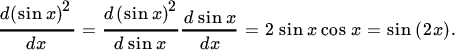
We now introduce the concept of a differential, by expressing (1) as
where we write d rather than d to emphasize that this is a differential rather than a derivative. The two concepts are closely related, but they are not the same.
The concept of differential may be confusing for students who remember their mathematics teacher explain to them that it is wrong to view dx2/dx as a fraction. They might wonder what dx and dx2 really are. What does dx2 = 2x dx mean? From a geometric point of view, it means that if we replace the graph of the function ϕ(x) = x2 at some value x by its linear approximation, that is, by the tangent line at the point (x, x2), then an increment dx in x leads to an increment dx2 = 2x dx in x2 in linear approximation. From an algebraic point of view, if we replace x by x + dx (‘increment dx’), then ϕ(x) is replaced by
For small dx, the term (dx)2 will be very small and, if we ignore it, we obtain the linear approximation x2 + 2x dx. The differential dx2 is, for a given value of x, just a function of the real variable dx, given by the formula dx2 = 2x dx.
This may sound complicated, but working with differentials is easy. The passage from ( 1 ) to (2) holds generally for any (differentiable) real‐valued function ϕ, and the differential dϕ is thus given by the formula
Put differently,
where α may depend on x, but not on dx. Equation (3) is a special case of the first identification theorem (Theorem 18.1) in the next section. It shows that we can identify the derivative from the differential (and vice versa), and it shows that the new concept differential is equivalent to the familiar concept derivative. We will always work with the differential, as this has great practical advantages.
The differential is an operator, in fact a linear operator, and we have
for any scalar constant a, and
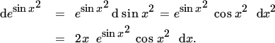
For the product and the ratio, we have
and, in addition to the differential of the exponential function dex = exdx,
The chain rule, well‐known for derivatives, also applies to differentials and is then called Cauchy's rule of invariance. For example,
or
or, combining the two previous examples,
The chain rule is a good example of the general principle that things are easier — sometimes a bit, sometimes a lot — in terms of differentials than in terms of derivatives. The chain rule in terms of differentials states that taking differentials of functions preserves composition of functions. This is easier than the chain rule in terms of derivatives. Consider, for example, the function z = h(x) = (sin x)2 as the composition of the functions
so that h(x) = f(g(x)). Then dy = cos x dx, and hence
as expected.
The chain rule is, of course, a key instrument in differential calculus. Suppose we realize that x in (4) depends on t, say x = t2. Then, we do not need to compute the differential of (sin t2)2 all over again. We can use ( 4 ) and simply write
The chain rule thus allows us to apply the rules of calculus sequentially, one after another.
In this section, we have only concerned ourselves with scalar functions of a scalar argument, and the reader may wonder why we bother to introduce differentials. They do not seem to have a great advantage over the more familiar derivatives. This is true, but when we come to vector functions of vector arguments, then the advantage will become clear.
3 VECTOR CALCULUS
Let x (n × 1) and y (m × 1) be two vectors and let y be a function of x, say y = f(x). What is the derivative of y with respect to x? To help us answer this question, we first consider the linear equation
where A is an m × n matrix of constants. The derivative is A and we write
The notation ∂f(x)/∂x′ is just notation, nothing else. We sometimes write the derivative as Df(x) or as Df, but we avoid the notation f′(x) because this may cause confusion with the transpose. The proposed notation emphasizes that we differentiate an m × 1 column vector f with respect to a 1 × n row vector x′, resulting in an m × n derivative matrix.
More generally, the derivative of f(x) is an m × n matrix containing all partial derivatives ∂fi(x)/∂xj, but in a specific ordering, namely
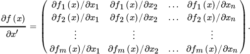
There is only one definition of a vector derivative, and this is it. Of course, one can organize the mn partial derivatives in different ways, but these other combinations of the partial derivatives are not derivatives, have no practical use, and should be avoided.
Notice that each row of the derivative in (6) contains the partial derivatives of one element of f with respect to all elements of x, and that each column contains the partial derivatives of all elements of f with respect to one element of x. This is an essential characteristic of the derivative. As a consequence, the derivative of a scalar function y = ϕ(x), such as y = a′x (where a is a vector of constants), is a row vector; in this case, a′. So the derivative of a′x is a′, not a.
The rules in the previous section imply that the following rules apply to vector differentials, where x and y are vectors and a is a vector of real constants, all of the same order:
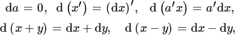
and
Now we can see the advantage of working with differentials rather than with derivatives. When we have an m × 1 vector y, which is a function of an n × 1 vector of variables x, say y = f(x), then the derivative is an m × n matrix, but the differential dy or df remains an m × 1 vector. This is relevant for vector functions, and even more relevant for matrix functions and for second‐order derivatives, as we shall see later. The practical advantage of working with differentials is therefore that the order does not increase but always stays the same.
Corresponding to the identification result ( 3 ), we have the following relationship between the differential and the derivative.
4 OPTIMIZATION
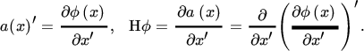
Let ϕ(x) be a scalar differentiable function that we wish to optimize with respect to an n × 1 vector x. Then we obtain the differential dϕ = a(x)′ dx, and set a(x) = 0. Suppose, for example, that we wish to minimize the function
where the matrix A is positive definite. The differential is
(Recall that a positive definite matrix is symmetric, by definition.) The solution ![]() needs to satisfy
needs to satisfy ![]() , and hence
, and hence ![]() . The function ϕ has an absolute minimum at
. The function ϕ has an absolute minimum at ![]() , which can be seen by defining
, which can be seen by defining ![]() and writing
and writing
Since A is positive definite, y′Ay has a minimum at y = 0 and hence ϕ(x) has a minimum at ![]() . This holds for the specific linear‐quadratic function (7) and it holds more generally for any (strictly) convex function. Such functions attain a (strict) absolute minimum.
. This holds for the specific linear‐quadratic function (7) and it holds more generally for any (strictly) convex function. Such functions attain a (strict) absolute minimum.
Next suppose there is a restriction, say g(x) = 0. Then we need to optimize subject to the restriction, and we need Lagrangian theory. This works as follows. First define the Lagrangian function, usually referred to as the Lagrangian,
where λ is the Lagrange multiplier. Then we obtain the differential of ψ with respect to x,
and set it equal to zero. The equations
are the first‐order conditions. From these n + 1 equations in n + 1 unknowns (x and λ), we solve x and λ.
If the constraint g is a vector rather than a scalar, then we have not one but several (say, m) constraints. In that case we need m multipliers and it works like this. First, define the Lagrangian
where l = (λ1, λ2, …, λm)′ is a vector of Lagrange multipliers. Then, we obtain the differential of ψ with respect to x:
and set it equal to zero. The equations
constitute n + m equations (the first‐order conditions). If we can solve these equations, then we obtain the solutions, say ![]() and
and ![]() .
.
The Lagrangian method gives necessary conditions for a local constrained extremum to occur at a given point ![]() . But how do we know that this point is in fact a maximum or a minimum? Sufficient conditions are available but they may be difficult to verify. However, in the special case where ϕ is linear‐quadratic (or more generally, convex) and g is linear, ϕ attains an absolute minimum at the solution
. But how do we know that this point is in fact a maximum or a minimum? Sufficient conditions are available but they may be difficult to verify. However, in the special case where ϕ is linear‐quadratic (or more generally, convex) and g is linear, ϕ attains an absolute minimum at the solution ![]() under the constraint g(x) = 0.
under the constraint g(x) = 0.
5 LEAST SQUARES
Suppose we are given an n × 1 vector y and an n × k matrix X with linearly independent columns, so that r(X) = k. We wish to find a k × 1 vector β, such that Xβ is ‘as close as possible’ to y in the sense that the ‘error’ vector e = y − Xβ is minimized. A convenient scalar measure of the ‘error’ would be e′e and our objective is to minimize
where we note that we write e′e/2 rather than e′e. This makes no difference, since any β which minimizes e′e will also minimize e′e/2, but it is a common trick, useful because we know that we are minimizing a quadratic function, so that a ‘2’ will appear in the derivative. The 1/2 neutralizes this 2.
Differentiating ϕ in (8) gives
Hence, the optimum is obtained when X′e = 0, that is, when ![]() , from which we obtain
, from which we obtain
the least‐squares solution.
If there are constraints on β, say Rβ = r, then we need to solve
We assume that the m rows of R are linearly independent, and define the Lagrangian
where l is a vector of Lagrange multipliers. The differential is
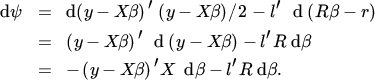
Setting the differential equal to zero and denoting the restricted estimators by ![]() and
and ![]() , we obtain the first‐order conditions
, we obtain the first‐order conditions
or, written differently,
We do not know ![]() but we know
but we know ![]() . Hence, we premultiply by R(X′X)−1. Letting
. Hence, we premultiply by R(X′X)−1. Letting ![]() as in (9), this gives
as in (9), this gives
Since R has full row rank, we can solve for l:
and hence for β:
Since the constraint is linear and the function ϕ is linear‐quadratic as in ( 7
), it follows that the solution![]() indeed minimizes ϕ(β) = e′e/2 under the constraint Rβ = r.
indeed minimizes ϕ(β) = e′e/2 under the constraint Rβ = r.
6 MATRIX CALCULUS
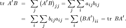
We have moved from scalar calculus to vector calculus, now we move from vector calculus to matrix calculus. When discussing matrices we assume that the reader is familiar with matrix addition and multiplication, and also knows the concepts of a determinant |A| and an inverse A−1. An important function of a square matrix A = (aij) is its trace, which is defined as the sum of the diagonal elements of A : tr A = ∑iaii. We have
which is obvious because a matrix and its transpose have the same diagonal elements. Less obvious is
for any two matrices A and B of the same order (but not necessarily square). This follows because
The rules for vector differentials in Section 3 carry over to matrix differentials. Let A be a matrix of constants and let α be a scalar. Then, for any X,
and, for square X,
If X and Y are of the same order, then
and, if the matrix product XY is defined,
Two less trivial differentials are the determinant and the inverse. For nonsingular X we have
and in particular, when |X| > 0,

The proof of (11) is a little tricky and is omitted (in this chapter, but not in Chapter 08).
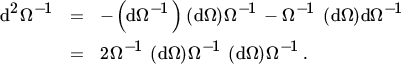
The differential of the inverse is, for nonsingular X,
This we can prove easily by considering the equation X−1X = I. Differentiating both sides gives
and the result then follows by postmultiplying with X−1.
The chain rule also applies to matrix functions. More precisely, if Z = F(Y) and Y = G(X), so that Z = F(G(X)), then
where A(Y) and B(X) are defined through
as in Theorem 18.2.
Regarding constrained optimization, treated for vector functions in Section 18.4, we note that this can be easily and elegantly extended to matrix constraints. If we have a matrix G (rather than a vector g) of constraints and a matrix X (rather than a vector x) of variables, then we define a matrix of multipliers L = (λij) of the same dimension as G = (gij). The Lagrangian then becomes
where we have used the fact, also used in (10) above, that
7 INTERLUDE ON LINEAR AND QUADRATIC FORMS
Before we turn from first to second differentials, that is, from linear forms to quadratic forms, we investigate under what conditions a linear or quadratic form vanishes. The sole purpose of this section is to help the reader appreciate Theorem 18.3 in the next section.
A linear form is an expression such as Ax. When Ax = 0, this does not imply that either A or x is zero. For example, if
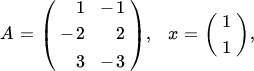
then Ax = 0, but neither A = 0 nor x = 0.
However, when Ax = 0 for every x, then A must be zero, which can be seen by taking x to be each elementary vector ei in turn. (The ith elementary vector is the vector with one in the ith position and zeros elsewhere.)
A quadratic form is an expression such as x′Ax. When x′Ax = 0, this does not imply that A = 0 or x = 0 or Ax = 0. Even when x′Ax = 0 for every x, it does not follow that A = 0, as the example
demonstrates. This matrix A is skew‐symmetric, that is, it satisfies A′ = −A. In fact, when x′Ax = 0 for every x then it follows that A must be skew‐symmetric. This can be seen by taking x = ei which implies that aii = 0, and then x = ei + ej which implies that aij + aji = 0.
In the special case where x′Ax = 0 for every x and A is symmetric, then A is both symmetric (A′ = A) and skew‐symmetric (A′ = −A), and hence A = 0.
8 THE SECOND DIFFERENTIAL
The second differential is simply the differential of the first differential:
Higher‐order differentials are similarly defined, but they are seldom needed.
The first differential leads to the first derivative (sometimes called the Jacobian matrix) and the second differential leads to the second derivative (called the Hessian matrix). We emphasize that the concept of Hessian matrix is only useful for scalar functions, not for vector or matrix functions. When we have a vector function f we shall consider the Hessian matrix of each element of f separately, and when we have a matrix function F we shall consider the Hessian matrix of each element of F separately.
Thus, let ϕ be a scalar function and let
where
The ijth element of the Hessian matrix Hϕ is thus obtained by first calculating aj(x) = ∂ϕ(x)/∂xj and then (Hϕ)ij = ∂aj(x)/∂xi. The Hessian matrix contains all second‐order partial derivatives ∂2ϕ(x)/∂xi ∂xj, and it is symmetric if ϕ is twice differentiable.
The Hessian matrix is often written as
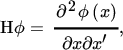
where the expression on the right‐hand side is a notation, the precise meaning of which is given by
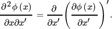
Given (13) and using the symmetry of Hϕ, we obtain the second differential as
which shows that the second differential of ϕ is a quadratic form in dx.
Now, suppose that we have obtained, after some calculations, that d2ϕ = (dx)′B(x) dx. Then,
for all dx. Does this imply that Hϕ = B(x)? No, it does not, as we have seen in the previous section. It does, however, imply that
and hence that Hϕ = (B(x) + B(x)′)/2, using the symmetry of Hϕ. This proves the following result.
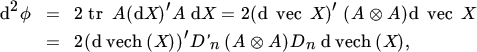
Alternatively — and this is often quicker — we differentiate ϕ twice without writing out the first differential in its final form. From
we thus obtain
which identifies the Hessian matrix as Hϕ = A + A′. (Notice that the matrix A in (16) is not necessarily symmetric.)
Even with such a simple function as ϕ(x) = x′Ax, the advantage and elegance of using differentials is clear. Without differentials we would need to prove first that ∂a′x/∂x′ = a′ and ∂x′Ax/∂x′ = x′(A + A′), and then use (15) to obtain

which is cumbersome in this simple case and not practical in more complex situations.
9 CHAIN RULE FOR SECOND DIFFERENTIALS
Let us now return to Example 18.2b. The function ϕ in this example is a function of x, and x is the argument of interest. This is why d2x = 0. But if ϕ is a function of x, which in turn is a function of t, then it is no longer true that d2x equals zero. More generally, suppose that z = f(y) and that y = g(x), so that z = f(g(x)). Then,
and
This is true whether or not y depends on some other variables. If we think of z as a function of y, then d2y = 0, but if y depends on x then d2y is not zero; in fact,
This gives us the following result.
In practice, one usually avoids Theorem 18.4 by going back to the first differential dz = A(y) dy and differentiating again. This gives (17), from which we obtain the result step by step.
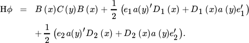
Having obtained the second differential in the desired form, Theorem 18.3 implies that the Hessian is equal to
10 FOUR EXAMPLES
Let us provide four examples to show how the second differential can be obtained. The first three examples relate to scalar functions and the fourth example to a matrix function. The matrix X has order n × q in Examples 18.5a and 18.6a, and order n × n in Examples 18.7a and 18.8a.
These four examples provide the second differential; they do not yet provide the Hessian matrix. In Section 18.14, we shall discuss the same four examples and obtain the Hessian matrices.
11 THE KRONECKER PRODUCT AND VEC OPERATOR
The theory and the four examples in the previous two sections demonstrate the elegance and simplicity of obtaining first and second differentials of scalar, vector, and matrix functions. But we also want to relate these first and second differentials to Jacobian matrices (first derivatives) and Hessian matrices (second derivatives). For this we need some more machinery, namely the vec operator and the Kronecker product.
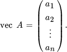
First, the vec operator. Consider an m × n matrix A. This matrix has n columns, say a1, …, an. Now define the mn × 1 vector vec A as the vector which stacks these columns one underneath the other:
For example, if
then vec A = (1, 4, 2, 5, 3, 6)′. Of course, we have
If A and B are matrices of the same order, then we know from ( 10 ) that tr A′B = ∑ijaijbij. But (vec A)′(vec B) is also equal to this double sum. Hence,
an important equality linking the vec operator to the trace.
We also need the Kronecker product. Let A be an m × n matrix and B a p × q matrix. The mp × nq matrix defined by
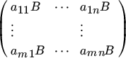
is called the Kronecker product of A and B and is written as A ⊗ B. The Kronecker product A ⊗ B is thus defined for any pair of matrices A and B, unlike the matrix product AB which exists only if the number of columns in A equals the number of rows in B or if either A or B is a scalar.
The following three properties justify the name Kronecker product:
if A and B have the same order and C and D have the same order (not necessarily equal to the order of A and B), and
if AC and BD exist.
The transpose of a Kronecker product is
If A and B are square matrices (not necessarily of the same order), then
and if A and B are nonsingular, then
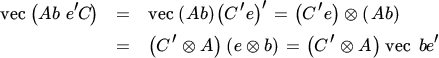
The Kronecker product and the vec operator are related through the equality
where a and b are column vectors of arbitrary order. Using this inequality, we see that
for any vectors b and e. Then, writing ![]() , where bj and ej denote the jth column of B and I, respectively, we obtain the following important relationship, which is used frequently.
, where bj and ej denote the jth column of B and I, respectively, we obtain the following important relationship, which is used frequently.
12 IDENTIFICATION
When we move from vector calculus to matrix calculus, we need an ordering of the functions and of the variables. It does not matter how we order them (any ordering will do), but an ordering is essential. We want to define matrix derivatives within the established theory of vector derivatives in such a way that trivial changes such as relabeling functions or variables have only trivial consequences for the derivative: rows and columns are permuted, but the rank is unchanged and the determinant (in the case of a square matrix) is also unchanged, apart possibly from its sign. This is what we need to achieve. The arrangement of the partial derivatives matters, because a derivative is more than just a collection of partial derivatives. It is a mathematical concept, a mathematical unit.
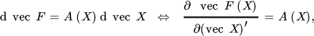
Thus motivated, we shall view the matrix function F(X) as a vector function f(x), where f = vec F and x = vec X. We then obtain the following extension of the first identification theorem:
and, similarly, for the second identification theorem:
where we notice, as in Section 18.8, that we only provide the Hessian matrix for scalar functions, not for vector or matrix functions.
13 THE COMMUTATION MATRIX
At this point, we need to introduce the commutation matrix. Let A be an m × n matrix. The vectors vec A and vec A′ contain the same mn elements, but in a different order. Hence, there exists a unique mn × mn matrix, which transforms vec A into vec A′. This matrix contains mn ones and mn(mn − 1) zeros and is called the commutation matrix, denoted by Kmn. (If m = n, we write Kn instead of Knn.) Thus,
It can be shown that Kmn is orthogonal, i.e. ![]() . Also, premultiplying (20) by Knm gives KnmKmn vec A = vec A, which shows that KnmKmn = Imn. Hence,
. Also, premultiplying (20) by Knm gives KnmKmn vec A = vec A, which shows that KnmKmn = Imn. Hence,
The key property of the commutation matrix enables us to interchange (commute) the two matrices of a Kronecker product:
for any m × n matrix A and p × q matrix B. This is easiest shown, not by proving a matrix identity but by proving that the effect of the two matrices on an arbitrary vector is the same. Thus, let X be an arbitrary q × n matrix. Then, by repeated application of ( 20 ) and Theorem 18.5,
Since X is arbitrary, (21) follows.
The commutation matrix has many applications in matrix theory. Its importance in matrix calculus stems from the fact that it transforms d vec X′ into d vec X. The simplest example is the matrix function F(X) = X′, where X is an n × q matrix. Then,
so that the derivative is D vec F = Knq.
The commutation matrix is also essential in identifying the Hessian matrix from the second differential. The second differential of a scalar function often takes the form of a trace, either tr A(dX)′ BdX or tr A(dX) BdX. We then have the following result, based on (19) and Theorem 18.5.
To identify the Hessian matrix from the first expression, we do not need the commutation matrix, but we do need the commutation matrix to identify the Hessian matrix from the second expression.
14 FROM SECOND DIFFERENTIAL TO HESSIAN
We continue with the same four examples as discussed in Section 18.10, showing how to obtain the Hessian matrices from the second differentials, using Theorem 18.6.
15 SYMMETRY AND THE DUPLICATION MATRIX
Many matrices in statistics and econometrics are symmetric, for example variance matrices. When we differentiate with respect to symmetric matrices, we must take the symmetry into account and we need the duplication matrix.
Let A be a square n × n matrix. Then vech(A) will denote the ![]() vector that is obtained from vec A by eliminating all elements of A above the diagonal. For example, for n = 3,
vector that is obtained from vec A by eliminating all elements of A above the diagonal. For example, for n = 3,
and
In this way, for symmetric A, vech(A) contains only the generically distinct elements of A. Since the elements of vec A are those of vech(A) with some repetitions, there exists a unique ![]() matrix which transforms, for symmetric A, vech(A) into vec A. This matrix is called the duplication matrix and is denoted by Dn. Thus,
matrix which transforms, for symmetric A, vech(A) into vec A. This matrix is called the duplication matrix and is denoted by Dn. Thus,
The matrix Dn has full column rank ![]() , so that
, so that ![]() is nonsingular. This implies that vech(A) can be uniquely solved from (23), and we have
is nonsingular. This implies that vech(A) can be uniquely solved from (23), and we have
One can show (but we will not do so here) that the duplication matrix is connected to the commutation matrix by
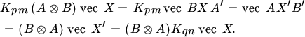
Much of the interest in the duplication matrix is due to the importance of the matrix ![]() , where A is an n × n matrix. This matrix is important, because the scalar function ϕ(X) = tr AX′AX occurs frequently in statistics and econometrics, for example in the next section on maximum likelihood. When A and X are known to be symmetric we have
, where A is an n × n matrix. This matrix is important, because the scalar function ϕ(X) = tr AX′AX occurs frequently in statistics and econometrics, for example in the next section on maximum likelihood. When A and X are known to be symmetric we have
and hence, ![]() .
.
From the relationship (again not proved here)
which is valid for any n × n matrix A, not necessarily symmetric, we obtain the inverse
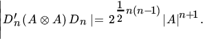
where A is nonsingular. Finally, we present the determinant:
16 MAXIMUM LIKELIHOOD
This final section brings together most of the material that has been treated in this chapter: first and second differentials, the Hessian matrix, and the treatment of symmetry (duplication matrix).
We consider a sample of m × 1 vectors y1, y2, …, yn from the multivariate normal distribution with mean μ and variance Ω, where Ω is positive definite and n ≥ m + 1. The density of yi is
and since the yi are independent and identically distributed, the joint density of (y1, …, yn) is given by ∏i f(yi). The ‘likelihood’ is equal to the joint density, but now thought of as a function of the parameters μ and Ω, rather than of the observations. Its logarithm is the ‘loglikelihood’, which here takes the form

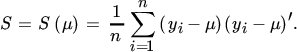
The maximum likelihood estimators are obtained by maximizing the loglikelihood (which is the same, but usually easier, as maximizing the likelihood). Thus, we differentiate Λ and obtain
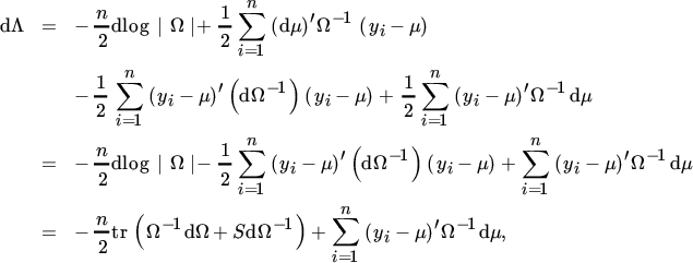
where
Denoting the maximum likelihood estimators by ![]() and
and ![]() , letting
, letting ![]() , and setting dΛ = 0 then implies that
, and setting dΛ = 0 then implies that
for all dΩ and
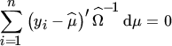
for all dμ. This, in turn, implies that
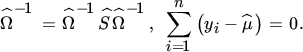
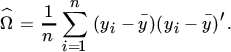
Hence, the maximum likelihood estimators are given by
and
We note that the condition that Ω is symmetric has not been imposed. But since the solution (28) is symmetric, imposing the condition would have made no difference.
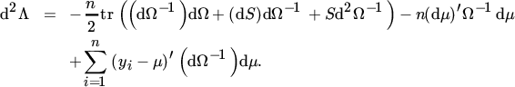
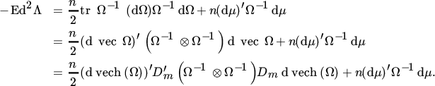
The second differential is obtained by differentiating (26) again. This gives
We are usually not primarily interested in the Hessian matrix but in its expectation. Hence, we do not evaluate (29) further and first take expectations. Since E(S) = Ω and E(dS) = 0, we obtain
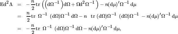
using the facts that dΩ−1 = −Ω−1 (dΩ)Ω−1 and
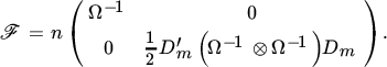
To obtain the ‘information matrix’ we need to take the symmetry of Ω into account and this is where the duplication matrix appears. So far, we have avoided the vec operator and in practical situations one should work with differentials (rather than with derivatives) as long as possible. But we cannot go further than (30) without use of the vec operator. Thus, from ( 30 ),
Hence, the information matrix for μ and vech(Ω) is
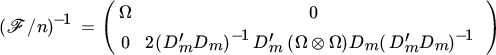
The results on the duplication matrix in Section 18.15 also allow us to obtain the inverse:
and the determinant:
FURTHER READING
2–3. Chapter 5 discusses differentials in more detail, and contains the first identification theorem (Theorem 5.6) and the chain rule for first differentials (Theorem 5.9), officially called ‘Cauchy's rule of invariance’.
4. Optimization is discussed in Chapter 07.
5. See Chapter 11, Sections 11.29–11.32 and Chapter 13, Sections 13.4 and 13.19.
6. The trace is discussed in Section 1.10, the extension from vector calculus to matrix calculus in Section 5.15, and the differentials of the determinant and inverse in Sections 8.3 and 8.4.
7. See Section 1.6 for more detailed results.
8–9. Second differentials are introduced in Chapter 06. The second identification theorem is proved in Section 6.8 and the chain rule for second differentials in Section 6.11.
11. See Chapter 2 for many more details on the vec operator and the Kronecker product. Theorem 2.2 is restated here as Theorem 18.5.
12. See Sections 5.15 and 10.2.
13 and §15. The commutation matrix and the duplication matrix are discussed in Chapter 03.
16. Many aspects of maximum likelihood estimation are treated in Chapter 15.