5.1 Introduction

In the analysis of variance, we assume that parameters of random variables depend on non‐random variables, called factors. The values a factor can take we call factor levels or in short levels. We discuss cases where one, two or three factors have an influence on the observations.

An experimenter often has to find out in an experiment whether different values of several variables or of several factors have different results on the experimental material. If the effects of several factors have to be examined, the conventional method means to vary only one of these factors at once and to keep all other factors constant. To investigate the effect of p factors this way, p experiments have to be conducted. It can be that the results at the levels of a factor investigated depend on the constant levels of other factors, which means that interactions between the factors exist. The British statistician R. A. Fisher recommended experimental designs by varying the levels of all factors at the same time. For the statistical analysis of the experimental results of such designs (they are called factorial experiments), Fisher developed a statistical procedure: the analysis of variance. The first publication about this topic stemmed from Fisher and Mackenzie (1923), a paper about the analysis of field trials in Fisher's workplace at Rothamsted Experimental Station in Harpenden, UK. A good overview is given in Scheffé (1959) and in Rasch and Schott (2018).

The analysis of variance is based on the decomposition of the sum of squared deviations of the observations from the total mean of the experiment into components. Each of the components is assigned to a specific factor or to interactions of factors or to the experimental error. Further, a corresponding decomposition of the degrees of freedom belonging to sums of squared deviations is done. The analysis of variance is mainly used to estimate the effects of factor levels or to test statistical hypotheses (model I in this chapter), or to estimate components of variance that can be assigned to the different factors (model II – see Chapter 6).

The analysis of variance can be applied to several problems based on mathematical models called model I, model II and the mixed model, respectively. The problem leading to model I is as follows: all factor levels have been particularly selected and involved in the experiment because just these levels are of practical interest. The objective of the experiment is to find out whether the effects of the different levels (or factor level combinations) differ significantly or randomly from each other. The experimental question can be answered by a statistical test if particular assumptions are fulfilled. The statistical conclusion refers to (finite) factor levels specifically selected.

In this chapter, problems in a model I are discussed and these are the estimation of the effects and the interaction effects of the several factors and testing the significance of these effects.

We also show how to determine the optimal size of an experiment. For all these cases we assume that we have to plan an experiment with a type I risk α = 0.05 and a power 1 − ß = 0.95.

 > install.packages("OPDOE")

and

 > library(OPDOE) 

 > help(size.anova) 

5.2 Planning the Size of an Experiment

For planning the size of a balanced experiment, this means equal sample sizes for the effects, precision requirements are needed, as in Chapter 3. The following approach is valid for all sections of this chapter. Besides the precision requirement of the two risks α and β (or the power of the F‐test 1 − β) the non‐centrality parameter λ of the non‐central F‐distribution with f₁ and f₂ degrees of freedom has to be given in advance. With the (1 − α)‐ and the β‐quantile of the non‐central F‐distribution with f₁ and f₂ degrees of freedom and the non‐centrality parameter λ we have to solve the equation

5.1

This equation plays an important role in all sections of this chapter. In addition to f₁, f₂, α, and β the difference δ between the largest and the smallest effect (main effect or in the following sections also interaction effect), to be tested against null, belongs to the precision requirement. We denote the solution λ in 5.1 by

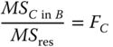
Let E_min, E_max be the minimum and the maximum of q effects E₁, E₂, … , E_q of a fixed factor E or an interaction, respectively. Usually we standardise the precision requirement by the relative precision requirement .

If E_max − E_min ≥ δ then for the non‐centrality parameter of the F‐distribution (for even q) with holds

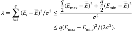
From this it follows

5.2

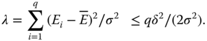
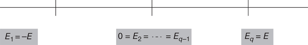
The minimal size of the experiment needed depends on λ accordingly to the exact position of all q effects. However, this is unknown when the experiment starts. We consider two extreme cases, the most favourable (resulting in the smallest minimal size n_min) and the least favourable (resulting in the largest minimal size n_max). The least favourable case leads to the smallest non‐centrality parameter λ_min and by this to the so‐called maximin size n_max. This occurs if the q − 2 non‐extreme effects equal . For this is shown in the following scheme.

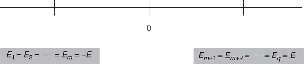
The most favourable case leads to the largest non‐centrality parameter λ_max and by this to the so‐called minimin size n_min. If q = 2m (even) this is the case, if m of the E_i equal E_min and the m other E_i equal E_max. If q = 2m + 1 (odd) again m of the E_i should equal E_min and m other E_i should equal E_max, and the remaining effect should be equal to one of the two extremes E_min or E_max. For this is shown in the following scheme for even q.

When we plan an experiment, we always obtain equal sub‐class numbers. Therefore, we use models and ANOVA tables mainly for the equal subclass number case because we then have simpler formulae for the expected mean squares. In the analysis programs, unequal sub‐class numbers are also possible.

In Section 5.3 we give a theoretical ANOVA – table (for random variables) with expected mean squares E(MS). To find a proper F‐statistic for testing a null hypothesis corresponding to a fixed row in the table we proceed as follows. If the null hypothesis is correct the numerator and denominator of F have the same expectation. In general it is a ratio of two MS of a particular null hypothesis with the corresponding degrees of freedom. This ratio is centrally F‐distributed if the numerator and the denominator in the case that the hypothesis is valid have the same expectation. This equality is, however, not sufficient if unequal subclass numbers occur, for instance it is not sufficient if the MS are not independent of each other. In this case, we obtain only a test statistic that is approximately F‐distributed. Such cases occur in Chapter 6. We write τ = δ/σ.

5.3 One‐Way Analysis of Variance

In this section, we investigate the effects of one factor.

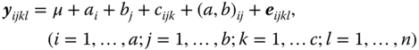
From a populations or universes, G₁, … , G_a random samples Y₁, … , Y_a of size n₁, … , n_a, respectively are drawn independently of each other. We write . The y_i are assumed to be distributed in the populations G_i as with {μ_i} = (μ_i, ⋯, μ_i)^T. Further we write μ_i = μ + a_i   (i = 1, … , a). Then we have one factor A with the factor levels A_i; i = 1,…, a and write

5.3

We call μ the total mean and a_i the effect of the ith level of factor A. The total size of the experiment is .

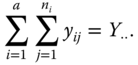
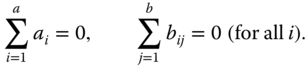
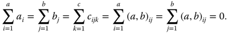
In Table 5.1, we find the scheme of the observations of an experiment with a levels A₁, ⋯, A_a of factor A and n_i observations for the ith level A_i of A. We use Equation 5.3 with the side conditions

	1	2	…	a
yij	y11 y12 ⋮	y21 y22 ⋮	⋯ ⋯ ⋮ ⋯	ya1 ya2 ⋮
ni Yi.	n1 Y1.	n2 Y2.	… …	na Ya.

For testing the hypothesis, e_ij and by this also y_ij is assumed to be normally distributed.

For testing hypotheses about μ + a_i further assumptions are not needed but to test hypotheses about a_i we need a so‐called reparametrisation condition like or ; both are equivalent if all n_i = n and this we call the balanced case.

In this chapter, we use the point convention for writing sums. In the one‐way case discussed in this section we have

and

The arithmetic means are and

Estimators for for μ in the model 5.3 are given by

5.4

5.5

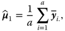
if we assume and by

5.6

5.7

if we assume . For estimable functions, we drop the left subscripts and write the symbols as in 5.3.

The n_i are called sub‐class numbers. Both estimators are identical in the balanced case if n_i = n (i = 1, … , a).

The reader may ask which reparametrisation condition he should use. There is no general answer. Besides the two forms above, many others are possible. However, fortunately many of the results derived below are independent of the side condition chosen. Often estimates of the a_i are less interesting than those for estimable functions of the parameters such as μ + a_i and a_i − a_j and these estimable functions give the same answer for all side conditions.

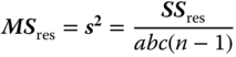
The variance σ² in both cases is unbiasedly estimated by

5.8

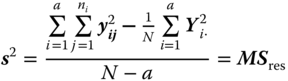
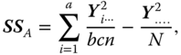
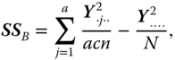
Table 5.2 gives the ANOVA table for model 5.3. In this table SS means sum of squares, MS means mean squares and df means degrees of freedom. We call this table a theoretical ANOVA table because we write the entries as random variables that are functions of the underlying random samples Y₁, … , Y_a. If we have observed data as realisations of the random samples then the column E(MS) is dropped and nothing in the table is in bold print.

Source of variation	SS	df	MS	E(MS) for ni = n
Main effect A		a−1
Residual		N−a		σ2

Table 5.3 is the empirical ANOVA table corresponding to Table 5.2.

Source of variation	SS	df	MS
Main effect A		a − 1
Residual		N − a
Total		N − 1

5.3.1 Analysing Observations

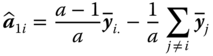
Estimable functions of the model parameters are for instance μ + a_i(i = 1, … , a) or a_i − a_j(i, j = 1, … , a; i ≠ j) with the estimators (using (5.4)–5.7)

5.9

and

5.10

respectively. They are independent of the special choice of the reparametrisation condition.

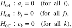
Besides point estimation, an objective of an experiment (model I) is to test the null hypothesis H₀ :  a_i = a_j for all i ≠ j against the alternative that at least two of the effects a_i differ from each other. This null hypothesis corresponds to the assumption that the effects of the factor considered for all a levels are equal. The basis of the corresponding tests is the fact that the sum of squared deviations SS of y_ij from the total mean of the experiment can be broken down into independent components.

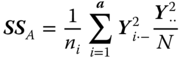
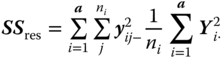
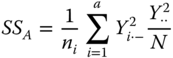
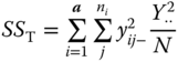
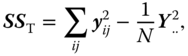
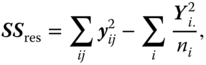
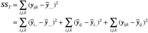
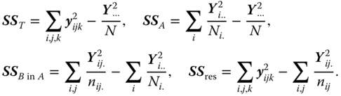
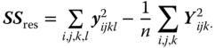
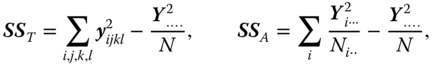
The total sum of squared deviations of the observations from the total mean of the experiment is

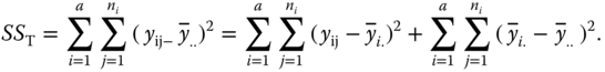
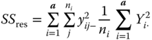
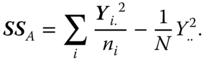
The left‐hand side is called SS total or for short SS_T, the first component of the right‐hand side is called SS within the treatments or levels of factor A (for short SS within SS_res) and the last component of the right hand side SS between the treatments or levels of factor A (SS_A), respectively.

We generally write

5.11

5.12

5.13

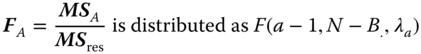
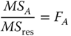
It is known from Rasch and Schott (2018, theorem 5.4) that

5.14

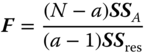
is distributed as F(a − 1, N − a, λ) with the non‐centrality parameter

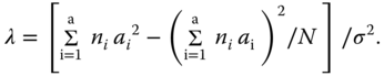
If H₀ :    a₁ =  …  = a_a is valid then we have λ = 0, and thus, F is F(a − 1,  N − a) distributed. Therefore, the hypothesis H₀: a₁ =  …  = a_a is tested by an F‐test. The ratios and are called mean squares between treatments and within treatments or residual mean squares, respectively.

5.4 Two‐Way Analysis of Variance

The two‐way ANOVA is a procedure for experiments to investigate the effects of two factors. Let us investigate a varieties of wheat and b fertilisers in their effect on the yield (kilogram per hectare). The a varieties as well as the b fertilisers are assumed to be fixed (selected consciously), as always in this chapter with fixed effects. One of the factors is factor variety (factor A), and the other factor is fertiliser (factor B). In this and the next chapter the number of levels of a factor X is denoted by the same (small) letter x as the factor (a capital letter) itself. So, factor A has a, and factor B has b levels in the experiment. In experiments with two factors, the experimental material is classified in two directions. For this, we list the different possibilities:

1. (a) Observations occur in each level of factor A combined with each level of factor B. There are a · b combinations (classes) of factor levels. We say factor A is completely crossed with factor B or that we have a complete cross‐classification.
   1. (a1) For each combination (class) of factor levels there exists one observation [(n_ij = 1 with n_ij being the number of observations in class (A_i. B_j).].
   2. (a2) For each combination (class) (i, j) the level i of factor A with the level j of factor B we have observations, with at least one n_ij > 1. If all n_ij = n, we have a cross‐classification with equal class numbers, called a balanced experimental design.
2. (b) At least one level of factor A occurs together with at least two levels of the factor B, and at least one level of factor B occurs together with at least two levels of the factor A, but we have no complete cross‐classification. Then we say factor A is partially crossed with factor B, or we have an incomplete cross‐classification.
3. (c) Each level of factor B occurs together with exactly one level of factor A. This is a nested classification of factor B within factor A. We also say that factor B is nested within factor A and write B ≺ A.

Summarising the types of two‐way classification we have:

1. (a) n_ij = 1 for all (i, j) → complete cross‐classification with one observation per class
2. (b) n_ij ≥ 1 for all (i,j) → complete cross‐classification
3. (c) n_ij = n ≥ 1 for all (i, j) → complete cross‐classification with equal sub‐class numbers
4. (d) At least one n_ij = 0 → incomplete cross‐classification.

If n_kj ≠ 0, then n_ij = 0 for i ≠ k (at least one n_ij > 1 and at least two n_ij ≠ 0) → nested classification.

5.4.1 Cross‐Classification (A × B)

The observations y_ijk of a complete cross‐classification are real numbers. In class (i,j) occur the observations y_ijk, k = 1, … , n_ij. In block designs, we often have n_ij = 1 with single subclass numbers. If all n_ij = n are equal, we have the case of equal subclass numbers, which we discuss now.

Without loss of generality, we represent the levels of factor A as the rows and the levels of factor B as the columns in the tables. When empty classes occur, i.e. some n_ij equal zero, we have an incomplete cross‐classification; such a case occurs for incomplete block designs.

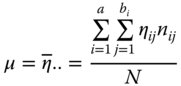
Let the random variables y_ijk in the class (i, j) be a random sample of a population associated with this class. The mean and variance of the population of such a class are called true mean and variance, respectively. The true mean of the class (i, j) is denoted by η_ij. Again we consider the case that the levels of the factors A and B are chosen consciously (model I).

We call

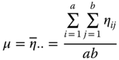
the overall expectation of the experiment.

The difference is called the main effect of the ith level of factor A, the difference is called the main effect of the j‐th level of factor B. The difference is called the effect of the ith level of factor A under the condition that factor B occurs in the jth level. Analogously, is called the effect of the jth level of factor B under the condition that factor A occurs in the ith level.

The distinction between the main effect and ‘conditional effect’ is important if the effects of the levels of one factor depend on the effect of the level of the other factor. In the analysis of variance, we then say that an interaction between the two factors exists. We define the effects of these interactions (and use them in place of the conditional results).

The interaction (a, b)_ij between the ith level of factor A and the jth level of factor B in a two‐way cross‐classification is the difference between the conditional effect of the level A_i of factor A for a given level B_j of the factors B and the main effect of the level A_i of A.

Under the assumption above the random variable y_ij of the cross‐classification varies randomly around the class mean in the form

We assume that the so‐called error variables e_ijk are independent of each other N(0, σ²) distributed and write for a balanced design the model I equation:

5.16

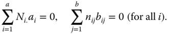
with (a, b)_ij = 0 if n = 0. We assume the following side conditions:

5.17

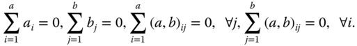
If in 5.14 all (a, b)_ij = 0 we call

5.18

a model without interactions or an additive model, respectively.

5.4.1.1 Parameter Estimation

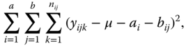
We can estimate the parameters in any model of ANOVA by the least squares method. We minimise in the case of model (5.16)

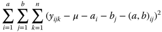
under the side conditions 5.17 and receive (using the dot convention analogue to Section 5.3)

5 Models with Interactions

We consider the model 5.15. Because E(Y) is estimable we have

estimable. The BLUE of η_ij is

5.19

From 5.6 it follows

5.20

It is now easy to show that differences between a_i or between b_j are not estimable. All estimable functions of the components of 5.15 without further side conditions contain interaction effects (a, b)_ij. It follows from theorem 5.7 in Rasch and Schott (2018) that

5.21

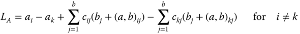
or analogously

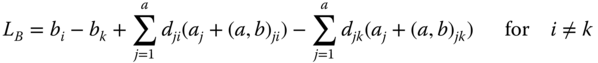
is estimable if c_rs = 0 for n_rs = 0 and d_rs = 0  for n_rs = 0 as well as

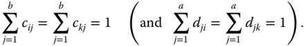
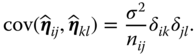
The BLUE of an estimable function of the form 5.21 is given by

5.22

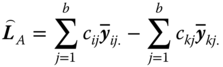
with variance

5.23

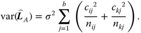
We consider the following example.

5 Connected Incomplete Cross‐Classifications

In an incomplete cross‐classification we have (a, b)_ij = 0 if n_ij = 0. Further we choose the factors A and B so that a ≥ b.

An (incomplete) cross‐classification is called connected if

is non‐singular. If |W| = 0, then the cross‐classification is disconnected.

5.4.1.2 Testing Hypotheses

In this section, testable hypotheses and tests of such hypotheses are considered.

5 Models without Interactions

We start with model 5.18 and assume a connected cross‐classification (W above non‐singular).

If, as in 5.18, n_ij = n (equal sub‐class numbers), simplifications for the tests of hypotheses about the main effects result. We have the possibility further to construct an analysis of variance table, in which SS_A, SS_B, SS_res = SS_R add to SS_total = SS_T.

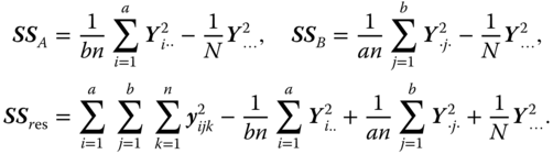
If in model 5.18 n ≥ 1 for all i and j, then the sum of squared deviations of the y_ijk from the total mean of the experiment

can be written as

with

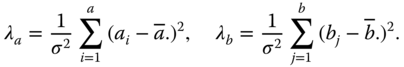
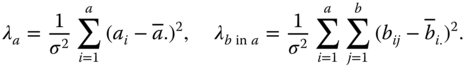
SS_A + SS_B and SS_res are independently distributed, and for normally distributed y_ijk we have distributed as CS(a − 1, λ_a), as CS(b − 1, λ_b) and as CS(N − a − b + 1) with non‐centrality parameters

Therefore, is non‐centrally F‐distributed with a − 1 and N − a − b + 1 degrees of freedom and non‐centrality parameter and is non‐centrally F‐distributed with b − 1 and N − a − b + 1 degrees of freedom and non‐centrality parameter .

The realisations of these formulas are summarised in Table 5.7.

Source of Variation	SS	df	MS	F
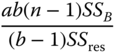
Between the levels of A		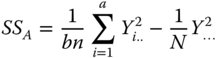a − 1
Between the levels of B		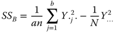b − 1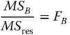
Residual	SSres = SST − SSA − SSB	N − a − b + 1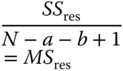

When the null hypothesis H_A0 : a₁ = a₂ =  ⋯  = a_a = 0 is correct, then λ_a = 0. This null hypothesis can therefore be tested by . If F_A > F(a − 1, N − a − b + 1, 1 − α) the null hypothesis is rejected with a first kind risk α. When the null hypothesis H_B0 : b₁ = b₂ =  ⋯  = b_b = 0 is correct, then λ_b = 0. This null hypothesis can therefore be tested by . If F_B > F(b − 1, N − a − b + 1, 1 − α) the null hypothesis is rejected with a first kind risk α.

Source of variation	SS	df	MS	F
Between the storages	43.2261	3	14.4087	186.7
Between the forage crops	0.8978	1	0.8978	11.63
Residual	0.2315	3	0.0772
Total	44.3554	7

5 Models with Interactions

We consider now model 5.16 and assume a connected cross‐classification.

The ANOVA table for this case is Table 5.10.

Source of variation	SS	df	MS	E(MS)	F
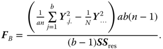
Between rows (A)		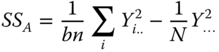a − 1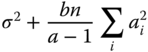
Between columns (B)		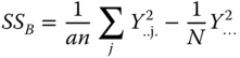b − 1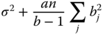
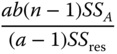
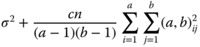
Interactions
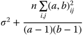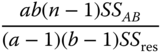Within classes (residual)		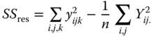ab(n − 1)		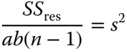σ2

In the case of equal subclass numbers, we use the side conditions 5.17 and test the hypotheses

with the F‐statistics

5.24

5.25

and

5.26

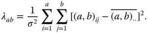
SS_A, SS_B, SS_AB and SS_res are independently distributed, and for normally distributed y_ijk it is as CS(a − 1, λ_a), as CS(b − 1, λ_b), as CS((a−1)(b − 1), λ_ab) and as CS(N − a − b + 1) distributed with non‐centrality parameters and , respectively.

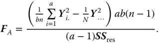
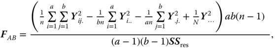
Therefore is non‐centrally F‐distributed with a − 1 and N − a − b + 1 degrees of freedom and non‐centrality parameter , is non‐centrally F‐distributed with b − 1 and N − a − b + 1 degrees of freedom and non‐centrality parameter and is non‐centrally F‐distributed with (a − 1)(b − 1) and N − a − b + 1 degrees of freedom and non‐centrality parameter

When the null hypotheses above are correct, then the corresponding non‐centrality parameter is zero. The corresponding null hypothesis can therefore be tested by , and , respectively. If F_A > F(a − 1, N − a − b + 1, 1 − α) the null hypothesis is rejected with a first kind risk α. If F_B > F(b − 1, N − a − b + 1, 1 − α) the null hypothesis is rejected with a first kind risk α. Finally, if F_AB > F((a − 1)(b − 1), N − a − b + 1, 1 − α) the null hypothesis H_A × B0 is rejected with a first kind risk α.

		Forage crop
Green rye	Lucerne
Kind of storage	Glass	8.39 7.68 9.46 8.12	9.44 10.12 8.79 8.89
Sack	5.42 6.21 4.98 6.04	5.56 4.78 6.18 5.91

Source of variation	SS	df	MS	F
Between the kind of storage	41.6347	1	41.6347	101.70
Between the forage crops	0.7098	1	0.7098	1.73
Interactions	0.9073	1	0.9073	2.22
Within classes (residual)	4.9128	12	0.4094
Total	48.1646	15

5.4.2 Nested Classification (A≻B)

A nested classification is a classification with super‐ and sub‐ordinated factors, where the levels of a sub‐ordinated or nested factor are considered as further subdivision of the levels of the super‐ordinated factor. Each level of the nested factor occurs in just one level of the super‐ordinated factor. An example is the subdivision of the United States into states (super‐ordinated factor A) and counties (nested factor B).

As for the cross‐classification we assume that the random variables y_ijk vary randomly from the expectations η_ij, i.e.

and that e_ijk are, independently of each other, N(0, σ²)‐distributed. With

the total mean of the experiment is defined.

In nested classification, interactions cannot occur.

The difference is called the effect of the ith level of factor A, the difference b_ij = η_ij − η_i. is the effect of the jth level of B within the ith level of A.

The model equation for y_ijk in the balanced case then reads

5.27

(interactions do not exist).

Usual side conditions are

or

5.28

Minimising

under the side conditions 5.28, we obtain the BLUE

5.29

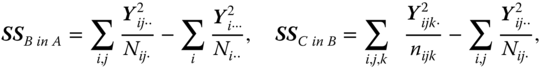
The total sum of squares is again split into components

or

where SS_A is the SS between the A levels, SS_{B in A} is the SS between the B levels within the A levels and SS_res is the SS within the classes (B levels).

The SS are written in the form

Here and in the sequel, we assume the side conditions 5.28.

The expectations of the MS are given in Table 5.13.

Source of variation	SS	df	MS	E(MS)
Between A levels		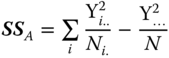a − 1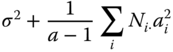
Between B levels within A levels		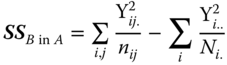B. − a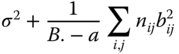
Within B levels (residual)		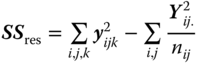N − B.		σ2

MS_A, MS_{B in A} and MS_res in Table 5.13 are independently of each other distributed as CS(a − 1, λ_a), CS(B. − a, λ_{b in a})  and CS(N − B.), respectively, where

Therefore

and

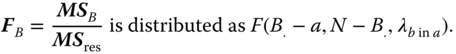
Using this the null hypothesis H_A0: a₁ =  …  = a_a, can be tested by , which, under H_A0 is distributed as F(a − 1, N − B_.).

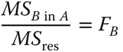
The null hypothesis H_B0: b₁₁ =  …  = b_ab, can be tested by , which, under H_B0, is distributed as F(B_. − a, N − B_.).

5.5 Three‐Way Classification

The principle underlying the two‐way ANOVA (two‐way classification) is also useful if more than two factors occur in an experiment. In this section, we only give a short overview of the cases with three factors without proving all statements because the principles of proof are similar to those in the case with two factors.

We consider the case with three factors because it often occurs in applications, which can be handled with a justifiable number of pages, and because besides the cross‐classification and the nested classification a mixed classification occurs. At this point, we make some remarks about the numerical analysis of experiments using ANOVA. Certainly, a general computer program for arbitrary classifications and numbers of factors with unequal class numbers can be elaborated. However, such a program, even with modern computers, is not easy to apply because the data matrices easily obtain several tens of thousands of rows. Therefore, we give for some special cases of the three‐way analysis of variance numerical solutions for which easy‐to‐use programs are written using R.

Problems with more than three factors are described in Hartung et al. (1997) and in Rasch et al. (2008).

5.5.1 Complete Cross‐Classification (A×B × C)

We assume that the observations of an experiment are influenced by three factors A, B, and C with a, b, and c levels A₁, … , A_a, B₁, … , B_b, and C₁, … , C_c, respectively. For each possible combination (A_i, B_j, C_k) let n ≥ 1 observations y_ijkl(l = 1, ⋯, n) be present. If the subclass numbers n_ijkl are not all equal or if some of them are zero but the classification is connected, we must use in R different models in >lm(). For the testing of interaction A × B, in the formula A × B must be placed before A × B × C; for the testing of interaction A × C, in the formula A × C must be placed before A × B × C; for the testing of interaction B × C in the formula B × C must be placed before A × B × C. An example of the analysis of an unbalanced three‐way cross‐classification with R is described at the end of this section.

Each combination (A_i, B_j, C_k) (i = 1, ⋯, a; j = 1, ⋯, b; k = 1, ⋯, c) of factor levels is called a class and is characterised by (i, j, k). The expectation in the population associated with the class (i, j, k) is η_ijk.

We define

and

The overall expectation is

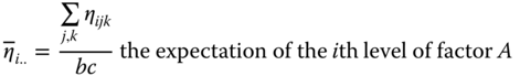
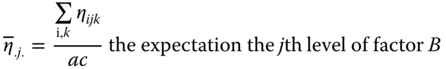
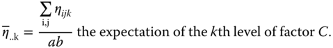
The main effects of the factors A, B, and C we define by

Assuming that the experiment is performed at a particular level C_k of the factor C we have a two‐way classification with the factors A and B, and the conditional interactions between the levels of the factors A and B for fixed k are given by

The interactions (a, b)_ij between the ith A level and the jth B level are the means over all C levels, i.e. (a, b)_ij is defined as

The interactions between A levels and C levels (a, c)_ik and between B levels and C levels (b, c)_jk are defined by

and

respectively.

The difference between the conditional interactions between the levels of two of the three factors for the given level of the third factor and the (unconditional) interaction of these two factors depends only on the indices of the levels of the factors, and not on the factor for which the interaction of two factors is calculated. We call it the second order interaction (a, b, c)_ijk (between the levels of three factors). Without loss of generality we write

The interactions between the levels of two factors are called first‐order interactions. From the definition of the main effect and the interactions we write for η_ijk

Under the definitions above, the side conditions for all values of the indices not occurring in the summation at any time are

The n observations y_ijkl in each class are assumed to be independent of each other and N(0, σ²)‐distributed. The variable (called error term) e_ijkl is the difference between y_ijkl and the expectation η_ijk of the class, i.e. we have

or

5.30

By the least squares method we obtain the following estimators:

as well as

If any of the interaction effects in 5.30 are zero the corresponding estimator above is dropped the others remain unchanged. The following model equations lead to different SS_res, as shown in Table 5.15.

5.31

Source of variation	SS	df
Between A levels		a − 1
Between B levels		b − 1
Between C levels		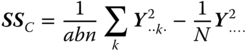c − 1
Interaction A  ×  B		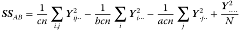(a − 1)(b − 1)
Interaction A  ×  C		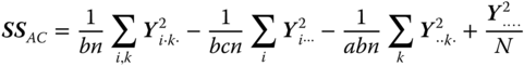(a − 1)(c − 1)
Interaction B  ×  C		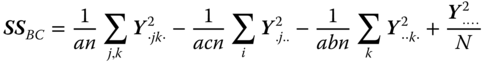(b − 1)(c − 1)
Interaction A  ×  B  ×  C		(a − 1)(b − 1)(c − 1)
Within the classes (residual), (5.30)		abc(n − 1)
Within the classes (residual), (5.31)		(a − 1)(b − 1) (c − 1) + abc(n − 1)
MS in (5.30)	E(MS) in (5.30)	F in (5.30)
	σ2

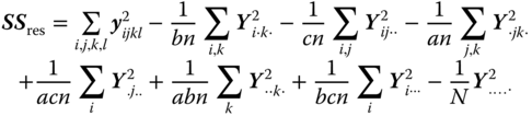
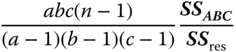
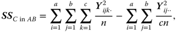
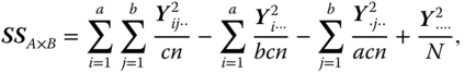
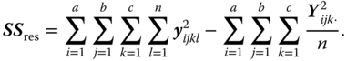
We may split the overall sum of squares into eight components: three corresponding with the main effects, three with the first order interactions, one with the second order interaction, and one with the error term or the residual. The corresponding SS are shown in the ANOVA table (Table 5.15). In this table N is, again, the total number of observations, N = abcn.

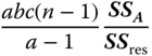
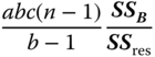
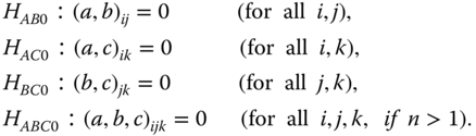
The following hypotheses can be tested (H_0x is one of the hypotheses H_0A, … , H_0ABC; SS_x is the corresponding SS).

Under the hypothesis are independent of each other, with the df given in the ANOVA table, centrally χ²‐distributed. Therefore, the test statistics given in column F of the ANOVA table are, with the corresponding degrees of freedom, centrally F‐distributed. For n = 1 all hypotheses except H_ABC0 can be tested under the assumption (a, b, c)_ijk = 0 for all i, j, k because then and , under H_x0(x = A, B, C,  etc.), are independent of each other centrally χ^2_‐distributed. The test statistic F_x is given by

If the null hypotheses are not true, we have non‐central distributions with non‐centrality parameters analogous to those in Section 5.4.

If the subclass numbers n_ijkl are not all equal or if some of them are zero but the classification is connected, we must change the formula for testing the two‐factor interactions. In the following example, we give an unbalanced three‐way cross‐classification.

5.5.2 Nested Classification (C ≺ B ≺ A)

We speak about a three‐way nested classification if factor C is sub‐ordinated to factor B and factor B is sub‐ordinated to factor A, i.e. if C ≺ B ≺ A. We assume that the random variable y_ijkl varies randomly with expected value η_ijk(i = 1, … , a; j = 1, … , b_i;  k = 1, … , c_ij), i.e. we assume

where e_ijkl, independent of each other, are N(0, σ²)‐distributed. Using

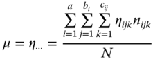
we define the total mean of the experiment as .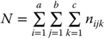

The difference is called the effect of the ith level of A, the difference is called the effect of the jth level of B within the ith level of A and the difference is called the effect of the kth level of C within the jth level of B and the ith level of A.

Then we model the observations using

5.32

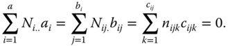
There exist no interactions. We consider 5.32 with under the side conditions

Minimising

5.33

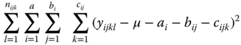
under the side conditions above, leads to the BLUE of the parameters as follows

In a three‐way nested classification we have

with 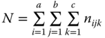, and

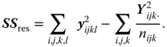
The variables up to are, with , pairwise independently CS(a − 1, λ_a),  CS(B. − a, λ_b), CS(C.. − B., λ_c), respectively, and is CS(N − C..)‐distributed. The non‐centrality parameters λ_a,  λ_b and λ_c vanish under the null hypotheses H_A0 :  a_i = 0 (i = 1, . … a), H_B0 :  b_ij = 0 (i = 1, . … a;  j = 1, … , b_i), H_C0 :  c_ijk = 0 (i = 1, . … a;  j = 1, … , b_i;  k = 1, … , c_ij), so that the usual F statistics can be used. Table 5.19 shows the SS and MS for calculating the F‐statistics. If H_A0 is valid F_A is F(a − 1,  N − C..)‐distributed. If H_B0 is valid then F_B is F(B − a,  N − C..)‐distributed, and if H_C0 is valid then F_c is F(C.. − B.,  N − C..)‐distributed.

Source of Variation	SS	df	MS	E(MS)	F
Between A		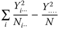a − 1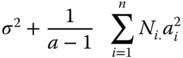
Between B in A		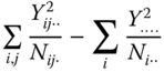B. − a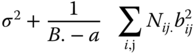
Between C in B and A		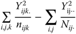C.. − B.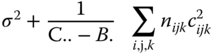
Residual		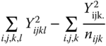N − C..		σ2
Total		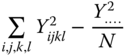N − 1

5.5.3 Mixed Classifications

In experiments with three or more factors besides a cross‐classification or a nested classification, we often find a further type of classification, the so‐called mixed (partially nested) classifications. In the three‐way ANOVA, two mixed classifications occur (Rasch 1971). We consider the case that the birth weight of piglets is observed in a three‐way classification with factors boar, sow within boar and gender of the piglet. The latter is cross‐classified with the nested factors boar and sow.

5.5.3.1 Cross‐Classification between Two Factors where One of Them Is Sub‐Ordinated to a Third Factor ((B ≺ A)xC)

If in a balanced experiment a factor B is sub‐ordinated to a factor A and both are cross‐classified with a factor C then the corresponding model equation is given by

5.34

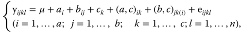
In 5.34 μ is the general experimental mean, a_i is the effect of the ith level of factor A; b_ij is the effect of the jth level of factor B within the ith level of factor A; c_k is the effect of the kth level of factor C. Further (a, c)_ik and (b, c)_jk(i) are the corresponding interaction effects and e_ijkl are the random error terms.

As usual, the error terms e_ijkl are independently distributed with expectation zero and the same variance σ²; for testing and confidence estimation normality is assumed in addition.

Model 5.34 is considered under the side conditions for all indices not occurring in the summation

5.35

and

5.36

(for all i,j, k, l).

The observations

are allocated as shown in Table 5.21 (we restrict ourselves to the so‐called balanced case where the number of B levels is equal for all A levels and the subclass numbers are equal).

	A1			A2
	B11	B12	B13	B21	B22	B23
C1	288 295	355 369	329 343	310 282	303 321	299 328
C2	278 272	336 342	320 315	288 287	302 297	289 284

5.5.3.2 Cross‐Classification of Two Factors, in which a Third Factor is Nested (C ≺ (A × B))

If two cross‐classified factors (A × B) are super‐ordered to a third factor (C) we have another mixed classification. The model equation for the random observations in a balanced design is given by

5.37

This is again the situation of model I; the error terms e_ijkl again fulfil condition 5.36.

We assume that for all values of the indices not occurring in the summation, we have the side conditions

5.38

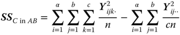
The total sum of squared deviations can be split into components

with

the SS between the A levels,

the SS between the B levels,

the SS between the C levels within the A × B combinations,

the SS for the interactions between factor A and factor B, and

The expectations of the MS in this model are shown in Table 5.23 and the hypotheses

Source of variation	SS
Between A levels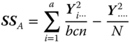
Between B levels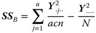
Between C levels in A × B combinations
Interaction A × B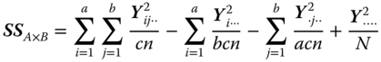
Residual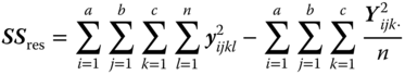
df	MS	E(MS) under (5.38)
a − 1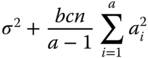
b − 1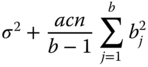
ab(c − 1)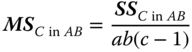
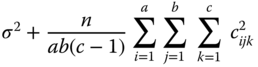(a − 1)(b − 1)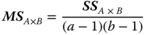
N − abc		σ2

H_A0 :    a_i = 0, H_B0 :    b_j = 0, H_C0 :    c_ijk = 0, H_AB0 :    (a, b)_ij = 0,

where the zero values are assumed to hold for all indices used in the hypotheses, can be tested by using the corresponding F‐statistic as the ratios of MS_A, MS_B, MS_C, and MS_A × B, respectively, (as numerator) and MS_res (as denominator).

References

1. Fisher, R.A. and Mackenzie, W.A. (1923). Studies in crop variation. II. The manurial response of different potato varieties. Journal of Agricultural Sciences 13: 311–320.
2. Hartung, J., Elpelt, B., and Voet, B. (1997). Modellkatalog Varianzanalyse. München: Oldenburg Verlag.
3. Kuehl, R.O. (1994). Statistical Principles of Research Design and Analysis. Belmont, California: Duxbury Press.
4. Lenth, R.V. (1986). Computing non‐central Beta probabilities. Appl. Statistics 36: 241–243.
5. Rasch, D. (1971). Mixed classification the three‐way analysis of variance. Biom. Z. 13: 1–20.
6. Rasch, D. and Schott, D. (2018). Mathematical Statistics. Oxford: Wiley.
7. Rasch, D., Wang, M., and Herrendörfer, G. (1997). Determination of the size of an experiment for the F‐test in the analysis of variance. Model I. In: Advances in Statistical Software 6. The 9th Conference on the Scientific Use of Statistical Software. Heidelberg: Springer.
8. Rasch, D., Herrendörfer, G., Bock, J., Victor, N., and Guiard, V. Hrsg. (2008). Verfahrensbibliothek Versuchsplanung und ‐ auswertung, 2. verbesserte Auflage in einem Band mit CD. R. Oldenbourg Verlag München Wien.
9. Rasch, D., Pilz, J., Verdooren, R., and Gebhardt, A. (2011). Optimal Experimental Design with R. Boca Raton: Chapman and Hall.
10. Scheffé, H. (1959). The Analysis of Variance. New York, Hoboken: Wiley.