3 Testing Hypotheses – One‐ and Two‐Sample Problems
3.1 Introduction
In empirical research, a scientist often formulates conjectures about objects of his research. For instance, he may argue that the fat content in the milk of Jersey cows is higher than that of Holstein Friesians. To check conjectures, he will perform an experiment. Now statistics come into play.
Sometimes the aim of investigation is not to determine certain statistics (to estimate parameters), but to test or to examine carefully considered hypotheses (assumptions, suppositions) and often also wishful notions based on practical material. In addition, in this case we establish a mathematical model where the hypothesis is formulated in the form of model parameters.
We assume that we have one random sample or two random samples from special distributions. We begin with the one‐sample problem and assume that the distribution of the components of the sample depends on a parameter (vector) θ. We would like to test a hypothesis about θ. First, we define what we have to understand by these terms.
A statistical test is a procedure that allows a decision for accepting or rejecting a hypothesis about the unknown parameter to occur in the distribution of a random variable. We shall suppose in the following that two hypotheses are possible. The first (or main) hypothesis is the null hypothesis H0, the other one is the alternative hypothesis HA. The hypothesis H0 is right, if HA is wrong, and vice versa. Hypotheses can be composite or simple. A simple hypothesis prescribes the parameter value θ uniquely, e.g. the hypothesis H0 : θ = θ0 is simple. A composite hypothesis admits that the parameter θ can have several values.
We discuss hypotheses testing based on random samples. A special random variable, a so‐called test statistic, is derived from the random sample. We reject the null hypothesis if the realisation of the test statistic has some relation to a real number; let us say it exceeds some quantile. This quantile is chosen so that the probability that the random test statistic exceeds it if the null hypothesis is correct is equal to a value 0 < α < 1; this is fixed in advance and is called the first kind risk or significance level. The first kind risk equals the probability to make an error of the first kind, i.e. to reject the null hypothesis if it is correct. Usually we choose α relatively small. From the time in which the quantiles mentioned above are calculated to produce tables – only for few values α‐quantiles did exist. From this time often α = 0.05 or 0.01 where used. However, even now it makes sense to use one of these values to make different experiments comparable.
Besides an error of the first kind, an error of the second kind may occur if we accept the null hypothesis although it is wrong; the probability that this occurs is the second kind risk.
Both errors have different consequences. Assume that the null hypothesis states that a special atomic power plant is safe. The alternative hypothesis is then that it is not safe. Of course, it is more harmful if the null hypothesis is erroneously accepted and the plant is assembled. Therefore, in this case the risk of the second kind is more important than the risk of the first kind. In many other cases, the risk of the first kind plays an important role and it is fixed in advance.
At the end of a classical statistical test we decide on one of two possibilities, namely accepting or rejecting the null hypothesis.
Tests for a given first kind risk α are called α‐tests; usually we have many α‐tests for a given pair of hypotheses. Amongst them, the ones that are preferable are those that have the smallest second kind risk β, or, equivalently, the largest power 1 − β. Such tests are called the most powerful α‐tests. When α ≤ β if HA is valid, the test is called unbiased.
A special situation arises in sequential testing. Here three decisions are possible after each of a series of sequentially registered observations:
accept H0
reject H0
make the next observation.
The value of the risk of the second kind depends on the distance between the parameter values of the null and the alternative hypothesis.
We need another term, the power function. This is the probability of rejecting H0. Its value equals α if the null hypothesis is correct.
It is completely wrong to state, after rejecting a null hypothesis based on observations, that this decision is wrong with probability α. This decision is either right or wrong. On the other hand, it is correct to say that the decision is based on a procedure, which supplies wrong rejections with probability α.
However, often a decision must be made.
Then one may say H0 is correct if accepting H0, even if this may be wrong.
Therefore, the user is recommended to choose α (or β, respectively) small enough that a rejection (or acceptance) of H0 allows the user to behave with a clear conscience, as H0 would be wrong (or HA right). However, there is also an important statistical consequence: if the user has to conclude many such decisions during his investigations, then he will wrongly decide in about 100α (and 100β, respectively) per cent of the cases. This is a realistic point of view, which essentially we have confirmed by experience. If we move in traffic, we should realise the risk of one's own and other people's incorrect actions or an accident (observe that in this case α is considerably smaller than 0.05), but we must participate, just as a researcher must derive a conclusion from an experiment, although he knows that he/she could be wrong. On the other hand, it is very important to control risks. Concerning risks of the second kind, this is only possible if the sample size is determined before the experiment. The user should take care not to transfer probability statements to single observed cases.
In this chapter, we discuss tests on expectations, variances, and other general parameters. Tests on special parameters like regression coefficients are found in the corresponding chapters.
Statistical tests and confidence estimations for expectations of normal distributions are extremely robust against the violation of the normality assumption – see Rasch and Tiku (1985).
3.2 The One‐Sample Problem
We begin with the one‐sample problem and assume that the distribution of the components of the sample depend on a parameter (vector) θ. We would like to test a hypothesis about θ. First, we define what we have to understand by these terms.
In this section we assume that a random sample Y = (y1, y2, … , yn)T, n ≥ 1 of size n is taken from a distribution with an unknown parameter. In Sections 3.2.1 and 3.2.3 we handle problems in which this distribution is a normal one with parameter vector .
3.2.1 Tests on an Expectation
We know simple and composite hypotheses.
In a simple hypothesis the value of θ = μ is fixed at a real number μ0.
A simple null hypothesis could be H0 : μ = μ0. In the pair H0 : μ = μ0; HA : μ = μ1 both hypotheses are simple.
Examples for composite null hypotheses are:
H0 : μ = μ0, σ2 arbitrary
H0 : μ = μ0 or μ = μ1
H0 : μ < μ0,
H0 : μ ≠ μ0.
3.2.1.1 Testing the Hypothesis on the Expectation of a Normal Distribution with Known Variance
We first assume that any component of Y = (y1, y2, … , yn)T is independently distributed as y, namely normally with unknown expectation μ and known variance σ2.
We like to test the null hypothesis
H0 : μ = μ0 against
(a)
HA : μ = μ1 > μ0 (one‐sided alternative)
(b)
HA : μ = μ1 < μ0 (one‐sided alternative)
(c)
HA : μ = μ1 ≠ μ0 (two‐sided alternative)
with a significance level α.
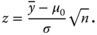
All hypotheses are simple hypotheses. In this case, usually the test statistic
3.1
is applied where is the mean taken from the random sample Y of size n.
Starting with the (random) sample mean first the value μ0 of the null hypothesis is subtracted and then this difference is divided by the standard error of .
We know that is normally distributed with variance 1 and, under the null hypothesis, the expectation of is 0. Under the alternative hypothesis the expectation of is . The value
3.2
is called the non‐centrality parameter (ncp) or, in applications, it is also called the relative effect size and δ = μ1 − μ0 is called the effect size.
We calculate from a realised sample, i.e. from observations Y = (y1, y2, … , yn)T, the sample mean following Problem 2.1 and from this the realised test statistic
3.3
Now we reject the null hypothesis for the alternative hypotheses (a), (b), and (c) with z from (3.3) and a fixed first kind risk or significance level α if:
(a)
z > Z(1 − α)
(b)
z < Z(α)
(c)
or .
Above Z(P), 0 < P < 1, is the P‐quantile of z, which has a standard normal distribution N(0,1).
3.2.1.2 Testing the Hypothesis on the Expectation of a Normal Distribution with Unknown Variance
We now assume that the components of a random sample Y = (y1, y2, … , yn)T are distributed normally with unknown expectation μ and unknown variance σ2.
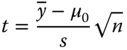
All hypotheses are composite hypotheses because σ2 is arbitrary. In this case, usually the test statistic (where s is the sample standard deviation):
3.6
is used which is non‐centrally t‐distributed with n − 1 degrees of freedom and ncp
Under the null hypothesis, the distribution is central t with n − 1 degrees of freedom.
If the type I error probability is α, H0 will be rejected if:
in case (a), t > t(n − 1;1 − α),
in case (b), t < −t(n − 1;1 − α),
in case (c),|t| > t(n − 1;1 − α/2).
Our precision requirement is given by α and the risk of the second kind β if μ − μ0 = δ.
From this we get
where t(n − 1;λ;β) is the β‐quantile of the non‐central t‐distribution with n − 1 degrees of freedom and ncp
For example, assuming a power of 0.9 the relative effect can be read on the abscissa; it is approximately 1.5 for n = 7.
From the precision requirement above the minimum sample size is iteratively determined as the integer solution of
3.7
(Rasch et al. 2011b) with P = 1 − α in the one‐sided case and P = 1 − α/2 in the two‐sided case. In Problem 3.3 it is shown what to do when σ is unknown.
In the command rdelta is equal to and p equals 1 − α. As an example we calculate
> size(p=0.9,rdelta=0.5,beta=0.1)[1] optimum sample number: n = 28.
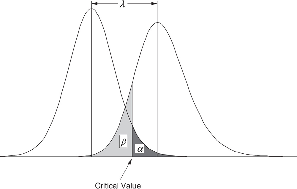
The requirement (3.7) is illustrated in Figure 3.2 for the one‐sided case.
Figure 3.2 Graphical representation of the two risks α and β and the non‐centrality parameter λ of a test based on (3.6).
3.2.2 Test on the Median
Sometimes the population median m should be preferred to the expectation of a random variable y. For any probability distribution of y on the real line R1with distribution function F(y), regardless of whether it is a continuous distribution or a discrete one, a median is by definition any real number m that satisfies the inequalities
If m is unique, the population median is the point where the distribution function equals 0.5.
It is better to use the median instead of the expectation if we expect serious outliers or if the distribution has an extremely skewness, so that in a sample the median better characterises the data than the mean. Tests on the population median are so‐called non‐parametric tests or distribution‐free tests. These are tests without a specific assumption about the distribution.
It is notable that such an approach is not intrinsically justified by a suspected deviation from the normal distribution of the character in question. Particularly as Rasch and Guiard (2004) showed that all tests based on the t‐distribution are extraordinarily robust against violations from the normal distribution. That is, even if the normal random variable is not a good model for the given character, the type I risk actually holds almost accurately. Therefore, if a test statistic results, on some occasions, in significance, we can be quite sure that an erroneous decision concerning the rejection of the null hypothesis has no larger risk than in the case of a normal distribution. We describe Wilcoxon's signed‐ranks test useful for continuous distributions.
We test the hypothesis
H0: m = m0 against a one‐ or two‐sided alternative:
HA: m < m0
HA: m > m0
HA: m≠m0.
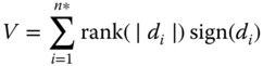
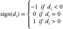
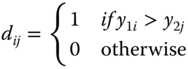
First, we calculate from each observation yi of a sample Y=(y1, y2, … , yn)T the differences di = yi − med(Y) between the observations and the median =med(Y) . If the value of di is equal to zero, we do not use these values. From the remaining data subset of size n* ≤ n the rank of the absolute values |di| is calculated. The sum,
3.9
with is the test statistic. Wilcoxon's signed‐ranks test is based on the distribution of the corresponding random variable, V.
Planning a study is generally difficult for non‐parametric tests, because it is hard to formulate a non‐centrality parameter (however see, for instance, Munzel and Brunner 2002).
3.2.3 Test on the Variance of a Normal Distribution
Equation (2.21) shows an unbiased estimator s2 of the variance σ2 of a normal distribution.
We would like to test the null hypothesis
against one of the alternatives below:
with a first kind risk α.
We know that
3.10
is centrally χ2 distributed with n − 1 degrees of freedom.
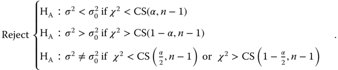
We calculate from a sample of size n the realisation of (3.10) and compare the result with the P‐quantile CS(P, n − 1) of the central χ2 distribution as follows:
3.11
3.2.4 Test on a Probability
We already discussed the analysis problem in Problem 3.5. Here we show how to determine the sample size approximately.
Let p be the probability of some event. To test one of the pairs of hypotheses below:
(a)
H0 : p ≤ p0, HA : p > p0
(b)
H0 : p ≥ p0, HA : p < p0
(c)
H0 : p = p0, HA : p ≠ p0
with a risk of the first kind α, and if we want the risk of the second kind to be not larger than β as long as
(a)
p1> p0, and p1 − p0 ≥ δ
(b)
p1< p0 and p0 − p1 ≥ δ
(c)
p0 ≠ p1 and |p0 − p1| ≥ δ.
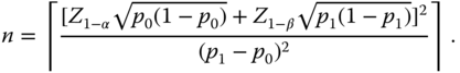
Determine the minimum sample size from
3.12
The same size is needed for the other one‐sided test. In the two‐sided case:
we replace α by α/2 and calculate (3.12) twice for p1 = p0 − δ > 0 and for p1 = p0 + δ < 1 if δ is the difference from p0, which should not be overlooked with a probability of at least 1 − β. From the two n‐values, we then take the maximum.
3.2.5 Paired Comparisons
If we measure two traits x and y from some individuals, we could say that we have a two‐sample problem. However, from a mathematical point of view we can say that the two measurements are realisations of a two‐dimensional random variable and from the corresponding universe one sample is drawn with measurements . We then speak about paired observations or statistical twins. In place of discussing the question of whether xi and yi have the same distribution we can ask whether the expectation of di= xi− yi is zero. The problem is reduced to that considered in Section 3.2.1 and must not be discussed again.
If the random variable d is extremely non‐normal (skew for instance) with the median m, then based on n realisations di, i = 1, … , n of the di null hypothesis, for the test below all di = 0 are excluded from the sample; the reduced sample size is denoted by n*.
H0 : m = m0 against HA : m ≠ m0 can be tested with Wilcoxon's signed rank test. For this the new differences are calculated as well as their absolute values after deleting the values 0. The remaining data set has a size n* ≤ n. Finally, these values are to be ordered (ascending) and ranks Ri are to be assigned accordingly.
Ties (identical values) receive a rank equal to the average of the ranks they span. The sum of the so‐called signed ranks is the test statistic of Wilcoxon's signed rank test. The corresponding random variable V has expectation E(V) = n*(n* + 1)/4 and variance . The null hypothesis H0 : m = m0 is rejected if V > V(n*, 1 − α), where α is the risk of the first kind. The critical values V(n*, 1 − α) are calculated by the R program in the following example.
3.2.6 Sequential Tests
The technique of sequential testing offers the advantage that, given many studies, on average fewer research units need to be sampled as compared to the ‘classic’ approach of hypothesis testing in Section 3.2.1 with sample size fixed beforehand.
Nevertheless, we need also the precision requirements α, β, and δ, moreover a sequential test cannot be applied without this, which means that we cannot start observations without fixing β. Until now a sample of fixed size n was given; Stein (1945) proposed a method of realising a two‐stage experiment. In the first stage a sample of size n0 > 1 is drawn to estimate σ2 using the variance of this sample and to calculate the sample size n of the method using (3.7). In the second stage n−no further measurements are taken. Following the original method of Stein in the second stage at least one further measurement is necessary from a theoretical point of view. In this section we simplify this method by introducing the condition that no further measurements are to be taken for n−no≤0. Nevertheless, this yields an α‐test of acceptable power.
Since both parts of the experiment are carried out one after the other, such experiments are called sequential. Sometimes it is even tenable to make all measurements step by step, where each measurement is followed by calculating a new test statistic. A sequential testing of this kind can be used if the observations of a random variable in an experiment take place successively in time. Typical examples are series of single experiments in a laboratory, psychological diagnostics in single sessions, medical treatments of patients in hospitals, consultations of clients of certain institutions, and certain procedures of statistical quality control, where the sequential approach was used the first time (Dodge and Romig 1929). The basic idea is to utilise the observations already made before the next are at hand.
For example, testing the hypothesis H0: μ = μ0 against HA: μ > μ0 (where the sample size can be determined by (3.7)) there are three possibilities in each step of evaluation, namely:
accept H0
reject H0
continue the investigation.
The, up to now unsurpassed, textbook of Wald (1947) has since been reprinted and is therefore generally available (Wald 2004), and new results can be found in the books of Ghosh and Sen (1991) and DeGroot (2005). We do not recommend the application of this general theory, but we recommend closed plans, which end after a finite number of steps with certainty (and not only with probability 1). We first give a general definition useful in other sections independent of our one‐sample problem.
3.3 The Two‐Sample Problem
We assume that two independent random samples from each of two populations are investigated.
Independent means that each outcome in one sample, as a particular event, will be observed independently of all outcomes in the other sample. Once the outcomes of the particular character are given, (point) estimates are calculated separately for each sample, as shown in Section 3.2. However, we discuss here the problem whether the two samples really stem from two different populations.
We will first consider again the parameter μ; that is, the two means of the two populations underlying the two samples.
3.3.1 Tests on Two Expectations
We assume that the character of interest is in each population modelled by a normally distributed random variable. That is to say, independent random samples of size n1 and n2, respectively, are drawn from populations 1 and 2. The observations of the random variables on the one hand and on the other hand will be and . We call the underlying parameters μ1 and μ2, and and , respectively. The unbiased estimators are then used for the expectations and , respectively, and for the variances and , respectively (according to Section 3.2).
We test the null hypothesis
H0: μ1 = μ2 = μ; against one of the alternative hypotheses
(a)
HA: μ1 < μ2
(b)
HA: μ1 > μ2
(c)
HA: μ1 ≠ μ2.
According to recent findings from simulation studies (Rasch et al. 2011a), the traditional approach is usually unsatisfactory because it is not theoretically regulated for all possibilities.
Nevertheless, we start with an introduction to the traditional approach because the current literature on applications of statistics refers to it, and methods for more complex issues are built on it. Further, there are situations in which it is certain that both populations have equal variances, especially if standardisation takes place, as in intelligence tests.
3.3.1.1 The Two‐Sample t‐Test
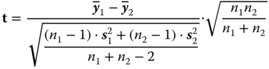
The traditional approach bases upon the test statistic in Formula (3.15). It examines the given null hypothesis for the case that the variances and , respectively, of the relevant variables in the two populations, are not known; this is the usual case. However, it assumes further that these variances are equal in both populations. The test statistic
3.15
is (central) t‐distributed with n1 + n2 − 2 degrees of freedom. This means, that we can decide in favour of, or against, the null hypothesis, analogous to Section 3.2, by using the (1 − α)‐quantile of the (central) t‐distribution t(n1 + n2 − 2, 1 − α) and t(n1 + n2 − 2, 1 − ), respectively, depending on whether it is a one‐ or two‐sided question.
H0: μ1 = μ2 = μ; will be rejected if:
(a)
t < t(n1 + n2 − 2, α)
(b)
t > t(n1 + n2 − 2, 1 − α)
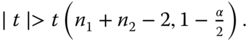
(c)
If the null hypothesis is rejected, we say that the two expectations differ significantly.
Thus, the minimum sample size for the one-sided case is 106, for the two-sided case we would need at least 121
observations each.
3.3.1.2 The Welch Test
We now discuss the case that either it is known that the variances and of the two populations are unequal or that we are not sure that they are equal – this is often the case. Therefore, we recommend always using the proposed Welch‐test below in place of the two‐sample t‐test. The recommendation to use the Welch test instead of the t‐test cannot be found in most textbooks of applied statistics and may therefore surprise experienced users. This recommendation is instead based on the results of current research from Rasch et al. (2011a). There it is also explained that pre‐testing first for equality of variances and if the equality is accepted to continue with the two‐sample t‐test makes no sense. We show in Table 3.5 a part of table 2 from Rasch et al. (2011a).
Table 3.5 A summary of a simulation study in Rasch et al. (2011a).
δ = 0
With pre‐tests
Without pre‐tests
√(σ21/σ22)
n1
n2
t
Welch (Levene)
W (KS)
t
Welch
W
1
10
10
4.95
4.55 (4.84)
0.00 (0.02)
4.96
4.82
5.21
30
30
4.97
4.82 (4.98)
11.11 (0.09)
4.96
4.95
4.92
10
30
5.00
4.87 (4.31)
0.00 (0.06)
5.01
5.05
4.87
30
10
4.97
5.09 (4.32)
0.00 (0.06)
4.96
5.15
5.00
30
100
4.86
5.00 (4.80)
9.09 (0.11)
4.84
4.91
4.82
2
10
10
6.08
3.33 (32.99)
0.00 (0.03)
5.38
4.93
6.06
30
30
7.37
4.78 (91.89)
10.00 (0.10)
5.15
4.98
5.88
10
30
1.02
5.90 (30.18)
0.00 (0.07)
0.90
5.00
2.19
30
10
19.38
2.98 (73.73)
16.67 (0.06)
15.51
5.19
10.09
30
100
1.33
4.99 (98.38)
0.00 (0.11)
0.63
4.96
1.89
The entries give the percentage of rejecting the (final) hypothesis H0: μ1= μ2. t is for student's t‐test and W for the Wilcoxon–Mann–Whitney‐test both with and without pre‐testing. Levene means the Levene test and KS the Kolmogorov–Smirnov test on normality.
Pre‐tests of the assumptions are worthless, as shown by our simulation experiments. First testing the normal assumption per sample, testing then the null hypothesis for equality of variances, with the Levene test from Section 3.3.4, and finally, testing the null hypothesis for equality of means leads to terrible risks, i.e. the risk estimated using simulation is only in the case of the Welch test near the chosen value α = 0.05 – it is exceeded by more than 20% in only a few cases. By contrast, the t‐test rejects the null hypothesis largely. Moreover, the Wilcoxon W‐test (see Section 3.3.1.3) does not maintain the type‐I risk in any way; it is too large and it has to be carried out with a newly collected pair of samples.
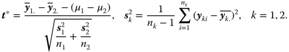
The Welch test is based on the test statistic
The distribution of the test statistic was derived by Welch (1947) and is presented in theorem 3.18 in Mathematical Statistics (Rasch and Schott, 2018).
If the pair of hypotheses
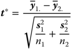
is to be tested, often the approximate test statistic
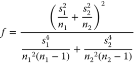
is used. H0 is rejected if |t*| is larger than the corresponding quantile of the central t‐distribution with approximate degrees of freedom f, the so‐called Satterthwaite's f,
degrees of freedom.
Referring to the t‐test, the desired relative effect size is, for equal sample sizes
For the Welch test, the desired relative effect size then reads:
Planning a study for the Welch test is carried out in a rather similar manner to that for two‐sample t‐test. A problem arises, however: in most cases it is not known whether the two variances in the relevant population are equal or not, and if not, to what extent they are unequal. If one knew this, then it would be possible to calculate the necessary sample size exactly. In the other case, one can use the largest appropriate size, which results from equal, realistically maximum expected variances.
3.3.1.3 The Wilcoxon Rank Sum Test
Wilcoxon (1945) proposed for equal sample sizes, and later Mann and Whitney (1947) extended for unequal sample sizes, a two‐sample distribution‐free test based on the ranks of the observations. This test is not based on the normal assumption, in its exact form only two continuous distributions with all moments existing are assumed; we call it the Wilcoxon test. As is seen from the title of Mann and Whitney (1947), this test is testing whether one of the underlying random variables is stochastically larger than the other. It can be used for testing the equality of medians under additional assumptions: if the continuous distributions are symmetric, the medians are equal to the expectations. The null hypothesis tested by the Wilcoxon test corresponds to the hypothesis of equality of the medians m1 and m2, H0 : m1 = m2 = m if and only if all higher moments of the two populations exist and are equal. Otherwise a rejection of the Wilcoxon hypothesis says little about the rejection of H0 : m1 = m2 = m. The test runs as follows based on the observations and of the random variables and respectively. We assume the sample size n1 ≤ n2.
Calculate:
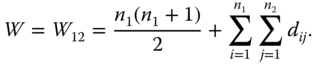
3.16
and
3.17
We denote the P‐quantiles of W based on n1 ≤ n2 observations by W(n1, n2, P).
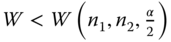
Reject H0:
in case (a), if W > W(n1, n2, 1 − α),
in case (b), if W < W(n1, n2, α),
in case (c), if either or ,
and accept it otherwise (the three cases are those given in problem 3.13).
The expectation of W if H0 is valid is E(W) = n1 (n1 + n2)/2.
The variance of W if H0 is valid is var(W) =n1n2(n1 + n2 + 1)/12.
Mann–Whitney used the test statistic U, which is the number of times that an x observation is larger than a y observation. The relation between U and W is: U = W −n1(n1 + 1)/2. Hence the expectation of U is E(U) = E(W) − n1(n1 + 1)/2 and the variance of U is var(U) = var(W −n1(n1 + 1)/2)
The expressions for var(W) and var(U) must be corrected if there are ties (equal observations) in the data.
If there are ties of size ti then var(W) must be subtracted by n1n2[Σ(ti3 − ti)]/[12(N2 − N)] and with ties we have var(W) = var(U) = {n1n2 (N3 − N − Σ(ti3 − ti)}/[12(N2 − N)].
The expectations of E(W) and E(U) remain the same in the case of ties.
Be aware that the quantiles of the random test statistic U are in R denoted by W and are given by the R‐command
3.3.1.4 Definition of Robustness and Results of Comparing Tests by Simulation
We give here an introduction to methods of empirical statistics via simulations and methods, which will be used later in this chapter and also in other chapters (especially in Chapter 11).
The robustness of a statistical method means that the essential properties of this method are relatively insensitive to variations of the assumptions. We especially want to investigate the robustness of the methods of this section with respect to violating normality.
3.3.1.5 Sequential Two‐Sample Tests
The technique of sequential testing offers the advantage that, given many studies, on average fewer research units need to be sampled as compared to the ‘classic’ approach of hypothesis testing in Sections 3.3.1.1–3.3.1.4 with sample sizes fixed beforehand. Nevertheless, we also need the precision requirements α, β, and δ. In the case of two samples from two populations and testing the null hypothesis H0: μ1 = μ2, a sequential triangular test is preferable. Its application is completely analogous to Section 3.2.5. The only difference is that we use δ = 0 − (μ1 − μ2) = μ2 − μ1 for the relevant (minimum difference) between the null and the alternative hypothesis, instead of δ = μ0 − μ. Again we keep on sampling data, i.e. outcomes, until we are able to make a terminal decision, namely to accept or to reject the null hypothesis.
3.3.2 Test on Two Medians
To test H0 whether two populations have the same median, against the alternative hypothesis HA that the medians are different, a random sample of size ni (i = 1,2) is drawn from each population. Be aware that the scale of the continuous measurement is at least ordinal, or else the term median is without meaning. A 2 × 2 contingency table is constructed, with rows ‘>median’ and ‘≤median’ and the columns for the sample i = 1, 2 of the two populations. The two entries in the ith column are the numbers of observations in the ith sample, which are above and below the combined sample grand median ; this is the median of all observations combined.
The median test has three appealing properties from the practical standpoint. In the first place it is primarily sensitive to differences in location between cells and not to the shapes of the cell distributions. Thus, if the observations of some cells were symmetrically distributed while in other cells they were positively skewed, the rank test would be inclined to reject the null hypothesis even though all population medians were the same. The median test would not be much affected by such differences in the shapes of the cell distributions. In the second place the computations associated with the median test are quite simple and the test itself is nothing more than the familiar contingency table test. In the third place when we come to consider more complex experiments it will be found that the median tests are not much affected by differing cell sizes. Bradley (1968) gives the following rationale and example for the Westenberg–Mood median test (Westenberg 1948; Mood 1950, 1954).
3.3.2.1 Rationale
Suppose that populations I and II are both continuously distributed populations of variate‐values, that the median variate‐value of the combined sample has the value , and that the two row categories are < and ≥, respectively. Then (if the number of observations in the combined sample is odd) the single observation equal to is excluded from all frequencies in the 2 × 2 table so that N (the total number of remaining data) is even, Fisher's exact method for the 2 × 2 contingency table becomes a test of hypotheses that equal but inexactly known proportions of populations I and II lie below (or if the original combined sample contained an even number of observations, below some population value lying between the [N/2]th and [(N/2) + 1]th observations in order of increasing size in the combined sample). Thus it tests the hypothesis that (or some value close to it) is the same, but unknown, quantile in the two populations; and if H0 is true and N is large the common proportion of the two populations lying below will tend to be close to 0.5, so will tend to be a population quantile, which is nearly a median. For this reason the Westenberg–Mood test is sometimes stated to attest to identical population medians; however, it is quite possible for two populations to have unequal medians and equal ‘ – quantiles’ or vice versa, especially when both samples are small. Instead of a median test, therefore, it might be better described as a quasi‐median test or a test for a common, probably more or less centrally located, quantile.
3.3.3 Test on Two Probabilities
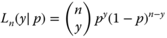
Let y be distributed as B(n, p). Knowing one observation y = Y we want to test H0: p = p0 against HA: p≠ p0, p0 ɛ (0, 1). The natural parameter is η =, and y is sufficient with respect to the family of binomial distributions. Therefore the uniformly most powerful unbiased (UMPU)‐α‐test is given by (3.27) in Rasch and Schott (2018), where the ciα and γ′iα (i = 1, 2) have to be determined from (3.28) and (3.29) in Rasch and Schott (2018). With
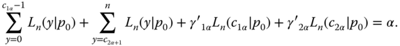
Equation (3.28) in Rasch and Schott (2018) has the form
3.20
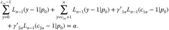
Regarding
the relation (3.29) in Rasch and Schott (2018) leads to
3.21
The solution of these two simultaneous equations can be obtained by statistical software, e.g. by R. Further results can be found in the book of Fleiss et al. (2003).
3.3.4 Tests on Two Variances
We consider two independent random samples , where the components yij are supposed to be distributed as N(μi). We intend to test the null hypothesis
against the alternative
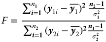
Under H0 we have = l, and the random variable
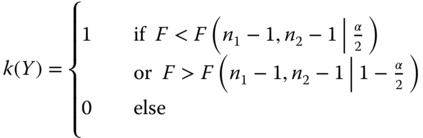
does not depend on μ1 and μ2, and . Since the random variable F is centrally distributed as F(n1 − 1, n2 − 1) under H0, the function
defines a UMPU‐α‐test, where F(n1 − 1, n2 − 1| P) is the P‐quantile of the F‐distribution with n1 − 1 and n2 − 1 degrees of freedom. This test is very sensitive to deviations from the normal distribution. Therefore the following Levene test should be used instead of it in the applications. Therefore we present no example or problem.
Instead we propose the Levene test. Box (1953) has already mentioned the extreme non‐robustness of the F‐test comparing two variances. Rasch and Guiard (2004) have reported on extensive simulation experiments devoted to this problem. The results of Box show that non‐robustness has to be expected already for relatively small deviations from the normal distribution. Hence, we generally suggest applying the test of Levene (1960) which is described now.
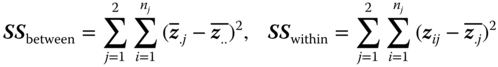
For j = 1, 2 we put
and
where .
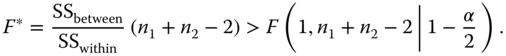
The null hypothesis H0 is rejected if
3.22
In R the Levene test is not available in the base package, but it is quite easy to program it yourself or it can be taken from the package car v3.0.0 by John Fox, see https://cran.r‐project.org/web/packages/car/car.pdf.
References
Box, G.E.P. (1953). Non‐normality and tests on variances. Biometrika 40: 318–335.
Bradley, J.V. (1968). Distribution‐Free Statistical Tests. Englewood Cliffs, New Jersey: Prentice‐Hall, Inc.
Dodge, H.F. and Romig, H.G. (1929). A method of sampling inspection. Bell Syst. Tech. J. 8: 613–631.
Fleishman, A.J. (1978). A method for simulating non‐normal distributions. Psychometrika 43: 521–532.
Fleiss, J.L., Levin, B., and Paik, M.C. (2003). Statistical Methods for Rates and Proportions, 3e. Hoboken: Wiley.
Ghosh, M. and Sen, P.K. (1991). Handbook of Sequential Analysis. Boca Raton: CRC Press.
Levene, H. (1960). Robust tests for equality of variances. In: Contributions to Probability and Statistics, 278–292. Stanford: Stanford University Press.
Mann, H.H. and Whitney, D.R. (1947). On a test whether one of two random variables is stochastically larger than the other. Ann. Math. Stat. 18: 50–60.
Mood, A.M. (1950). Introduction to the Theory of Statistics. New York: McGraw‐Hill.
Mood, A.M. (1954). On asymptotic efficiency of certain nonparametric two‐sample tests. Ann. Math. Stat. 25: 514–533.
Munzel, U. and Brunner, E. (2002). An exact paired rank test. Biom. J. 44: 584–593.
Rasch, D. and Guiard, V. (2004). The robustness of parametric statistical methods. Psychol. Sci. 46: 175–208.
Rasch, D. and Schott, D. (2018). Mathematical Statistics. Oxford: Wiley.
Rasch, D. and Tiku, M.L. (eds. 1985). Robustness of statistical methods and nonparametric statistics Proc. Conf. on Robustness of Statistical Methods and Nonparametric Statistics, Schwerin (DDR), May 29–June 2, 1983. Reidel Publishing Company Dordrecht.
Rasch, D., Kubinger, K.D., and Moder, K. (2011a). The two‐sample t test: pre‐testing its assumptions does not pay‐off. Stat. Pap. 52: 219–231.
Rasch, D., Pilz, J., Verdooren, R., and Gebhardt, A. (2011b). Optimal Experimental Design with R. Boca Raton: Chapman and Hall.
Rasch, D., Kubinger, K.D., and Yanagida, T. (2011c). Statistics in Psychology Using R and SPSS. Hoboken: Wiley.
Stein, C. (1945). A two sample test for a linear hypothesis whose power is independent of the variance. Ann. Math. Stat. 16: 243–258.
Wald, A. (1947). Sequential Analysis. New York: Dover Publ.
Wald, A. (2004). Sequential Analysis Reprint. New York: Wiley.
Welch, B.L. (1947). The generalization of students problem when several different population variances are involved. Biometrika 34: 28–35.
Westenberg, J. (1948). Significance test for median and interquartile range in samples from continuous populations of any form. Proc. Koninklijke Nederlandse Akademie van Wetenschappen, (The Netherlands) 51: 252–261.
Whitehead, J. (1997). The Design and Analysis of Sequential Clinical Trials, 2e Revised. New York: Wiley.
Wilcoxon, F. (1945). Individual comparisons by ranking methods. Biom. Bull. 1: 80–82.
 or
or  .
.
 is the test statistic. Wilcoxon's signed‐ranks test is based on the distribution of the corresponding random variable, V.
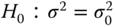 against one of the alternatives below:

 or
or 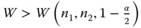 ,
,