Chapter 18
Showing Relationships between Continuous Dependent and Categorical Independent Variables
IN THIS CHAPTER
![]() Running an inferential test
Running an inferential test
![]() Comparing means
Comparing means
![]() Comparing independent-samples
Comparing independent-samples
![]() Graphing means
Graphing means
![]() Comparing independent-samples summary statistics
Comparing independent-samples summary statistics
![]() Comparing paired-samples
Comparing paired-samples
In this chapter, we explain how to compare different groups on a continuous outcome variable. For example, you can compare the money spent on rent by residents of two cities to determine if significant differences exists. You also learn how to compare the same group of people that have been assessed at two different time points or conditions, such as before and after an intervention.
Conducting Inferential Tests
In Chapter 16, we discuss how to conduct inferential tests for one variable. However, most statistical tests involve at least two variables: the dependent (effect) and independent (cause) variables.
The independent variable is the variable that the researcher controls or that is assumed to have a direct effect on the dependent variable. The dependent variable is the variable measured in research, that is, affected by the independent variable. For example, if you are testing the effect of a drug on depression, drug type is the independent variable and depression symptom is the dependent variable. Table 18-1 shows some appropriate statistical techniques based on the measurement level of the dependent and independent variables.
TABLE 18-1 Level of Measurement and Statistical Tests for Two or More Variables
|
Dependent Variables |
Independent Variables |
|
Categorical |
Continuous |
|
|
Categorical |
Crosstabs, nonparametric tests |
Logistic regression, discriminant analysis |
|||
|
Continuous |
T-test, analysis of variance (ANOVA) |
Correlation, linear regression |
|||
In Chapter 17, we discuss the crosstabs procedure, which is used when both the independent and dependent variables are categorical. In this chapter, we discuss t-tests, which are used when the independent variable is categorical and the dependent variable is continuous. In Chapter 19, we discuss correlation and simple linear regression, which are used when both the independent and dependent variables are continuous. In Part 6, we briefly discuss some additional advanced statistical techniques.
Using the Compare Means Dialog
Often, you encounter situations where you have a continuous dependent variable and a categorical independent variable. For example, you may want to determine if differences in SAT scores exist according to sex. Or you may want to see if there was a change in behavior by assessing someone before and after an intervention. In both examples, you’re comparing groups on some continuous outcome measure, and the statistic you’re using to make comparisons between groups is the mean. For this type of analysis, you use the procedures in the Compare Means dialog, shown in Figure 18-1. The Compare Means dialog (which is accessed by choosing Analyze ⇒ Compare Means) contains six statistical techniques that allow users to compare sample means:
- Means: Calculates subgroup means and related statistics for dependent variables within categories of one or more independent variables.
- One-sample t-test: Tests whether the mean of a single variable differs from a specified value (for example, a group using a new learning method compared to the school average). See Chapter 16 for an example.
- Independent-samples t-test: Tests whether the means for two different groups differ on a continuous dependent variable (for example, females versus males on income).
- Summary independent-samples t-test: Uses summary statistics to test whether the means for two different groups differ on a continuous dependent variable (for example, females versus males on income).
- Paired-samples t-test: Tests whether the means of the same group differ under two conditions or time points (for example, assessing the same group of people before versus after an intervention or under two distinct conditions, such as standing versus sitting).
- One-way ANOVA: Tests whether the means for two or more different groups differ on a continuous dependent variable (for example, drug1 versus drug2 versus drug3 on depression). See Chapter 20 for an example.
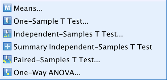
FIGURE 18-1: The Compare Means dialog.
Running the Independent-Samples T-Test Procedure
In this section, you focus on the independent-samples t-test, which allows you to compare two different groups on a continuous dependent variable. For example, you might be comparing two different learning methods to determine their effect on math skills.
Here’s how to perform an independent-samples t-test:
-
On the main menu, choose File ⇒ Open ⇒ Data and load the Employee_data.sav file.
You can download the file from the book’s companion website at
www.dummies.com/go/spss4e. The file contains employee information from a bank in the 1960s and has 10 variables and 474 cases. -
Choose Analyze ⇒ Compare Means ⇒ Independent-Samples T Test.
The Independent-Samples T Test dialog appears.
-
Select the Current Salary, Beginning Salary, Months since Hire, Educational Level, and Previous Experience variables, and place them in the Test Variable(s) box.
Continuous variables are placed in the Test Variable(s) box.
-
Select the gender variable and place it in the Grouping Variable box.
Categorical independent variable are placed in the Grouping Variable box. Note that you can have only one independent variable and that the program requires you to indicate which groups are to be compared.
-
Click the Define Groups button.
The Define Groups dialog appears.
-
In the Group 1 box, type 0; in the Group 2 box, type 1 (see Figure 18-2).
 If the independent variable is continuous, you can specify a cut point value to define the two groups. Cases less than or equal to the cut point go into the first group, and cases greater than the cut point are in the second group. Also, if the independent variable is categorical but has more than two categories, you can still use it by specifying only two categories to compare in an analysis.
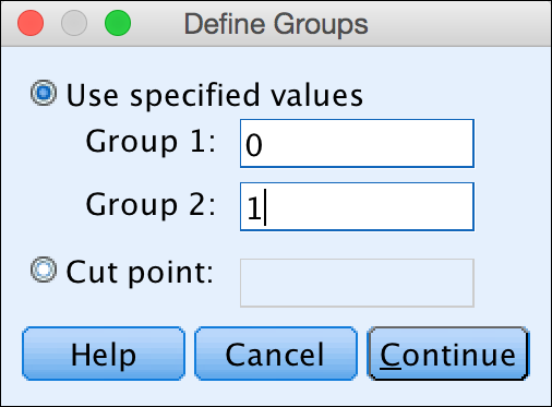
FIGURE 18-2: The Define Groups dialog.
-
Click Continue.
You’re returned to the Independent-Samples T Test dialog (shown in Figure 18-3).
You can also click the Options button and decide how to treat missing values and confidence intervals.
- Click OK.
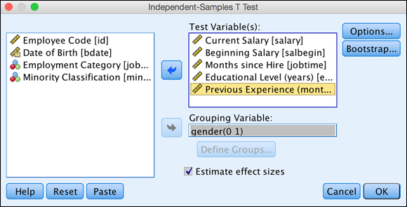
FIGURE 18-3: The Independent-Samples T Test dialog, with the Grouping Variable box completed.
 Every statistical test has assumptions. The better you meet these assumptions, the more you can trust the results of the test. The independent-samples t-test has four assumptions:
- The dependent variable is continuous.
- Only two different groups are compared.
- The dependent variable is normally distributed within each category of the independent variable (normality).
- Similar variation exists within each category of the independent variable (homogeneity of variance).
The purpose of the independent samples t-test is to test whether the means of two separate groups differ on a continuous dependent variable and, if so, whether the difference is significant. Going back to the idea of hypothesis testing, you can set up two hypotheses:
- Null hypothesis: The means of the two groups will be the same.
- Alternative hypothesis: The means of the two groups will differ from each other.
The Group Statistics table shown in Figure 18-4 provides sample sizes, means, standard deviations, and standard errors for the two groups on each of the dependent variables. You can see that the sample has a few more males (258) than females (216), but you're certainly not dealing with small sizes.
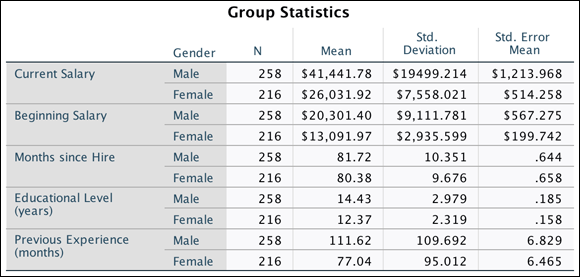
FIGURE 18-4: The Group Statistics table.
The independent-samples t-test works well even when you have moderate violations of the assumption of normality as long as the sample sizes are at least moderate (more than 50 cases per group), which is what you have in this situation. When we describe tests in which you can get away with moderate violations, we often use the term robust. Some tests can be more robust than others, and some assumptions can be more robust than others. There is even a category of tests called collectively robust tests.
In this example, you can see that males have higher means than females on all dependent variables. This is precisely what the independent-samples t-test assesses — whether the differences between the means are significantly different or if the differences are due to chance.
The Independent Samples Test table shown in Figure 18-5 displays the result of the independent-samples t-test. Before you look at this test, you must determine if you met the assumption of homogeneity of variance.
 The assumption of homogeneity of variance says that similar variation exists within each category of the independent variable — in other words, the standard deviation of each group is similar. Violating the assumption of homogeneity of variance is more critical than violating the assumption of normality, because when the former occurs, the significance or probability value reported by SPSS is incorrect and the test statistics must be adjusted.
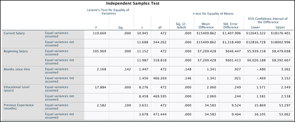
FIGURE 18-5: The Independent Samples Test table.
Levene’s test for equality of variances assesses the assumption of homogeneity of variance. This test determines if the variation is similar or different between the groups. When Levene’s test is not statistically significant (that is, the assumption of equal variance was met), you can continue with the regular independent-samples t-test and use the results from the Equal Variances Are Assumed row.
When Levene’s test is statistically significant (that is, the assumption of equal variance was not met), differences in variation exist between the groups, so you have to make an adjustment to the independent-samples t-test. In this situation, you would use the results from the Equal Variances Are Not Assumed row. Note that if the assumption of homogeneity of variance is not met, you can still do the test but must apply a correction.
In the left section of the Independent Samples Test table, Levene’s test for equality of variances is displayed. The F column displays the actual test result, which is used to calculate the significance level (the Sig. column).
In the example, the assumption of homogeneity of variance was met for the Months Since Hire and Previous Experience variables because the value in the Sig. column is greater than 0.05 (no difference exists in the variation of the groups). Therefore, you can look at the row that specifies that equal variances are assumed. However, the assumption of homogeneity of variance was not met for the Educational Level, Current Salary, and Beginning Salary variables because the value in the Sig. column is less than 0.05 (a difference exists in the variation of the groups). Therefore, you have to look at the row that specifies that equal variances are not assumed.
Now that you've determined whether the assumption of homogeneity of variance was met, you're ready to see if the differences between the means are significantly different or are due to random variation. The t column displays the result of the t-test and the df column tells SPSS Statistics how to determine the probability of the t-statistic. The Sig. (2-tailed) column tells you the probability of the null hypothesis being correct. If the probability value is very low (less than 0.05), you can conclude that the means are significantly different.
In Figure 18-5, you can see that significant differences exist between males and females on all variables except Months Since Hire. Thus, you can conclude that for the sample, males had significant higher beginning and current salary than females. Males also had more years of education and previous work experience than females. However, no difference exists in the amount of time that females and males had worked at the bank.
An additional piece of useful information is the 95 percent confidence interval for the population mean difference. Technically, this tells you that if you were to continually repeat this study, you would expect the true population difference to fall within the confidence intervals 95 percent of the time. From a more practical standpoint, the 95 percent confidence interval provides a measure of the precision with which the true population difference is estimated.
In the example, the 95 percent confidence interval for the mean difference between groups on years of education ranges from 1.581 to 2.538 years; the actual mean difference is 2.06 years of education. So the 95 percent confidence interval indicates the likely range within which you expect the population mean difference to fall. In this case, the value is 2.06, but you are 95 percent confident that the education difference value will fall anywhere between 1.581 to 2.538 years — basically the mean difference +/- the standard error of the difference (.249) multiplied by 1.96.
Note that the confidence interval does not include zero because a statistically significant difference exists between groups. If zero had been included within the range, it would indicate no differences between the groups — that is, the probability value is greater than 0.05.
In essence, the 95 percent confidence interval is another way of testing the null hypothesis. If the value of zero does not fall within the 95 percent confidence, the probability of the null hypothesis being true (that is, no difference or a difference of zero) is less than 0.05.
For each t-test, Figure 18-6 shows the effect sizes, which indicate the strength of the relationship between variables or the magnitude of the difference between groups. Cohen’s d is one of the most popular effect size measures; other measures of effect size are also available.
 Cohen’s d was just added to version 27 of SPSS. If you have an earlier version of the software, you will not have this output.
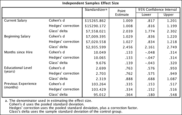
FIGURE 18-6: The Independent Samples Effect Size table.
Effect sizes do vary by research field. To get a general sense of effect sizes, you can use Table 18-2 as a guideline. In the example, you can see that the effect sizes for both beginning and current salary are quite large because the values are bigger than 0.8.
TABLE 18-2 Cohen’s d Effect Size Measure
|
Effect |
Value |
|
|
Small |
0.2 |
|
|
Medium |
0.5 |
|
|
Large |
0.8 |
|
Comparing the Means Graphically
For presentations, it's often useful to show a graph of the results of an independent samples t-test. The most effective way to do this when comparing means is to use a simple error bar chart, which focuses more on the precision of the estimated mean for each group than the mean itself.
Next, you create an error bar chart corresponding to the independent-samples t-test of gender and number of years of education. To see how the number of years of education varies across categories of gender, you'll use education as the Y-axis variable.
Follow these steps to create a simple error bar chart:
-
From the main menu, choose File ⇒ Open ⇒ Data and load the Employee_data.sav data file.
You can download the file at
www.dummies.com/go/spss4e. - Choose Graphs ⇒ Chart Builder.
- In the Choose From list, select Bar.
- Select the seventh graph image (the one with the Simple Error Bar tooltip) and drag it to the panel at the top of the window.
- Select the Educational Level variable, and place it in the Y-axis box.
- Select the Gender variable, and place it in the X-axis box.
-
Click OK.
The graph in Figure 18-7 appears.
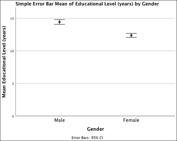
FIGURE 18-7: A simple error bar graph displaying the relationship between years of education and gender.
The error bar chart generates a graph depicting the relationship between a scale and a categorical variable. It provides a visual sense of how far the groups are separated.
The mean number of years of education for each gender along with 95 percent confidence intervals is represented in this chart. The confidence intervals for the two genders don't quite overlap, which is consistent with the result from the t-test and indicates that the groups are significantly different from each other. Also, the error bars have a small range compared to the range of years of education, which indicates that you're fairly precisely estimating the mean number of years of education for each gender (because of large sample sizes).
Running the Summary Independent-Samples T-Test Procedure
The summary independent-samples t-test procedure, like the independent-samples t-test procedure, performs an independent-samples t-test. However, the independent-samples t-test procedure requires you to have all your data to run the analysis (SPSS is reading your data directly from Data Editor). In the summary independent-samples t-test procedure, however, you specify only the number of cases, the means, and the standard deviations for each group to run the analysis.
The summary independent-samples t-test procedure is a Python extension and is available only if you allow Python extensions to be installed either during the SPSS installation process or at a later point.
The summary independent-samples t-test procedure is useful when it’s too time-consuming to enter all the data in the SPSS Data Editor window. With this technique, you can quickly obtain means and standard deviations using a calculator and then run a t-test. Or you can use this procedure to replicate the results of a published study for which you don’t have the data.
To perform the summary independent-samples t-test procedure, follow these steps:
-
From the main menu, choose File ⇒ Open ⇒ Data and load the Employee_data.sav file.
You can download the file at
www.dummies.com/go/spss4e. -
Choose Analyze ⇒ Compare Means ⇒ Summary Independent-Samples T Test.
The T Test Computed from Summary Data dialog appears. You want to study whether there are differences between two samples. You need to specify the number of cases in each group, along with the respective means and standard deviations.
- In the Number of Cases boxes under both Sample 1 and Sample 2, type 50.
- In the Mean box for Sample 1, type 4.2; in the Mean box for Sample 2, type 3.5.
-
In the Standard Deviation box for Sample 1, type 1.6; in the Standard Deviation box for Sample 2, type 1.5.
The completed dialog is shown in Figure 18-8.
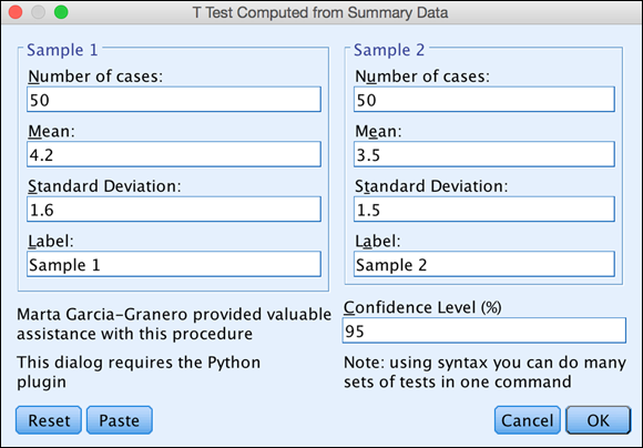
FIGURE 18-8: The completed T Test Computed from Summary Data dialog.
-
Click OK.
SPSS calculates the summary independent-samples t-test.
The Summary Data table shown in Figure 18-9 provides sample sizes, means, standard deviations, and standard errors for the two groups. You provided this summary information to perform the analysis.
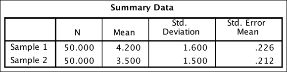
FIGURE 18-9: The Summary Data table.
The Independent Samples Test table shown in Figure 18-10 displays the result of the independent-samples t-test, along with the Hartley test of equal variance (which, like Levene’s test, assesses the assumption of homogeneity of variance). In the example, the assumption of homogeneity of variance was met because the Sig. value for Hartley’s test is greater than 0.05. Therefore, use the Equal Variances Are Assumed row. At this point, you're ready to see if the differences between the means are significantly different or due to chance.
As before, the t column displays the result of the t-test and the df column tells SPSS how to determine the probability of the t-statistic. The Sig. (2-tailed) column tells you the probability of the null hypothesis being correct. If the probability value is very low (less than 0.05), you can conclude that the means are significantly different. In Figure 18-10, you can see that significant differences exist between the samples.
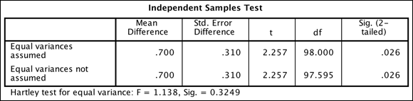
FIGURE 18-10: The Independent Samples Test table.
The final table, 95.0% Confidence Intervals for Difference (shown in Figure 18-11), displays the 95 percent confidence intervals for the population mean difference. As mentioned, confidence intervals tell you that if you were to continually repeat this study, you would expect the true population difference to fall within the confidence intervals 95 percent of the time.
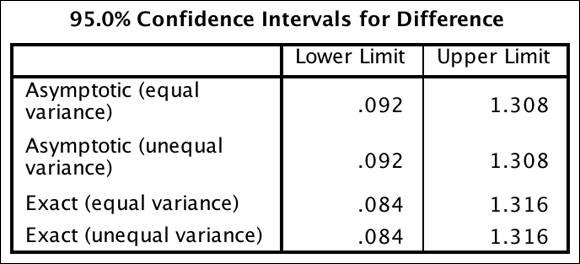
FIGURE 18-11: The 95.0% Confidence Intervals for Difference table.
Similar to the preceding example, you have confidence intervals for when the assumption of homogeneity of variance is met and not met. However, now you have the option to use asymptotic (an approximation) or exact (the exact value) confidence intervals, whereas in the preceding example you had to use asymptotic confidence intervals. The exact 95 percent confidence interval for the mean difference between groups is from 0.84 to 1.316. Because the difference values don’t include zero, there is a difference between groups.
Running the Paired-Samples T-Test Procedure
In this section, you focus on the paired-samples t-test, which tests whether the means of the same group differ on a continuous dependent variable under two different conditions or time points. For example, a paired-samples t-test could be used in medical research to compare means on a measure administered both before and after some type of treatment. In market research, if participants rated on some attribute a product they usually purchase and a competing product, a paired-samples t-test could compare the mean ratings. In customer satisfaction studies, if a special customer care program were implemented, you could test the level of satisfaction before and after the program was in place.
The goal of the paired-samples t-test is to determine if a significant difference or change from one time point or condition to another exists. To the extent that an individual's outcomes across the two conditions are related, the paired-samples t-test provides a more powerful statistical analysis (greater probability of finding true effects) than the independent-samples t-test because each person serves as his or her own control.
Going back to the idea of hypothesis testing, you can set up two hypotheses:
- Null hypothesis: The mean of the difference or change variable will be zero.
- Alternative hypothesis: The mean of the difference or change variable will not be zero.
Follow these steps to perform a paired-samples t-test:
-
From the main menu, choose File ⇒ Open ⇒ Data and load the Employee_data.sav file.
Download the file at
www.dummies.com/go/spss4e. This file contains employee information from a bank in the 1960s and has 10 variables and 474 cases. -
Choose Analyze ⇒ Compare Means ⇒ Paired-Samples T Test.
The Paired-Samples T Test dialog appears.
-
Select the Current Salary and Beginning Salary variables, and place them in the Paired Variables box (see Figure 18-12).
These variables are now in the same row, so they will be compared.
Technically, the order in which you select the pair of variables does not matter. The calculations will be the same. However, SPSS subtracts the second variable from the first. So in terms of presentation, you might want to be careful how SPSS displays the results so as to facilitate reader understanding. - Click OK.
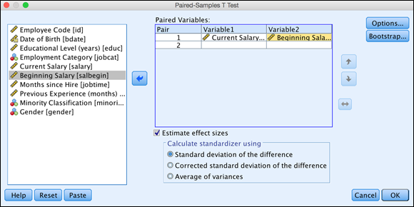
FIGURE 18-12: The Paired-Samples T Test dialog, with variables selected.
Every statistical test has assumptions. The better you meet these assumptions, the more you can trust the results of the test. The paired-samples t-test has three assumptions:
- The dependent variable is continuous.
- The two time points or conditions that are compared are on the same continuous dependent variable. In other words, the dependent variable should be measured in a consistent format: not, for example, on a seven-point scale the first time and then on a ten-point scale the second time.
- The difference scores are normally distributed (normality).
The Paired Samples Statistics table shown in Figure 18-13 provides sample sizes, means, standard deviations, and standard errors for the two time points. You can see that 474 people were in this analysis, with an average beginning salary of about $17,016 and average current salary of about $34,419.
As with the independent-samples t-test, the paired-samples t-test also works well even when you have moderate violations of the assumption of normality as long as sample sizes are at least moderate (more than 50 cases per group), which is what you have in this situation.
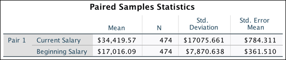
FIGURE 18-13: The Paired Samples Statistics table.
The Paired Samples Correlations table shown in Figure 18-14 displays the sample size (number of pairs) along with the correlation between the two variables. (See Chapter 19 for a discussion of correlations.) The higher the correlations, the more likely you are to detect a mean difference if differences exist. The correlation (.88) is positive, high, and statistically significant (differs from zero in the population), which suggests that the power to detect a difference between the two means is substantial.
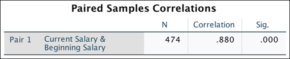
FIGURE 18-14: The Paired Samples Correlations table.
The null hypothesis is that the two means are equal. The mean difference in current salary compared to beginning salary is about $17,403. The Paired Samples Test table in Figure 18-15 reports this along with the sample standard deviation and standard error.
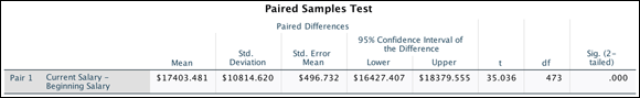
FIGURE 18-15: The Paired Samples Test table.
The t column displays the result of the t-test and the df column tells SPSS Statistics how to determine the probability of the t-statistic. The Sig. (2-tailed) column tells you the probability of the null hypothesis being correct. If the probability value is very low (less than 0.05), you can conclude that the means are significantly different. You can see that there are significant differences between the means. Thus, you can conclude that current salary is significantly higher than beginning salary.
As with the independent-samples t-test, the 95 percent confidence interval provides a measure of the precision with which the true population difference is estimated. In the example, the 95 percent confidence interval indicates the likely range within which you expect the population mean difference to fall. In this case, the mean difference value is about $17,403, but you are 95 percent confident that the true difference in change in salary will fall anywhere between $16,427 to $18,379, which is basically the mean difference +/- the standard error of the difference ($497) multiplied by 1.96. Again, note that the confidence interval does not include zero because a statistically significant difference between the time point exists.
Figure 18-16 shows the effect sizes for the t-test. As mentioned, effect sizes indicate the strength of the relationship between variables or the magnitude of the difference between groups. The value of the effect size is found in the Point Estimate column. (As mentioned, you can get a sense of effect sizes by using Table 18-1.) In the example, you can see that the effect size is very large because the value is larger than 0.8.
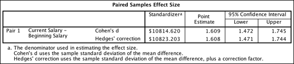
FIGURE 18-16: The Paired Samples Effect Size table.