Chapter 8
The Transform and Data Menus
IN THIS CHAPTER
![]() Sorting your cases in different ways
Sorting your cases in different ways
![]() Using some data (and not other data)
Using some data (and not other data)
![]() Combining counting and case identifying
Combining counting and case identifying
![]() Recoding variable content to new values
Recoding variable content to new values
![]() Grouping data in bins
Grouping data in bins
After you get your raw data into SPSS, you may find that it contains errors or isn’t organized how you’d like. A way to alleviate these problems is to make modifications to your data by configuring the values into a form that’s easier to work with and read. This chapter contains some methods you can use to modify your data without losing any information.
A related problem occurs when you want to analyze only some of your data or perform the same analysis more than once. For example, you may want to select the good, complete data and avoid the incomplete, messy data. Or you may want to do a separate analysis for new customers and established customers.
Sorting Cases
You can change the order of your cases (rows) so they appear in just about any order you want. You sort them by comparing the values you entered for your variables. The following example uses the Cars.sav dataset. You sort with two variables, or sort keys. The initial sort of the data will simply be by car_id.
 You don't need to limit your sorting to one or two sort keys. You can have a third key or more, if necessary, but these keys come into effect only when the keys sorted before them hold identical values. In most cases, two sort keys are enough to get what you want.
You can sort based on variables of any type simply by selecting the variables as keys. For example:
-
Choose File ⇒ Open ⇒ Data and select the Cars.sav file.
The file is not in the SPSS installation directory. You have to download it from the book’s companion website at
www.dummies.com/go/spss4e. The result is the presentation of a collection of apparently unsorted cases, as shown in Figure 8-1.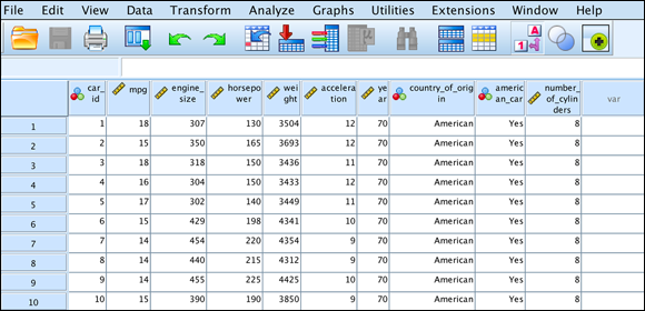
FIGURE 8-1: The data unsorted, as it's loaded directly from the data file.
-
Choose Data ⇒ Sort Cases.
The Sort Cases dialog appears.
-
Select the
country_of_originvariable and then thehorsepowervariable, in that order, and either click the arrow button or drag the variables to the Sort By box, as shown in Figure 8-2. The order of the sort keys is important. If you had chosen
 Horsepowerfirst andCountry_of_Originsecond, the results would have been different. -
Click OK to sort the data.
The result is shown in Figure 8-3.
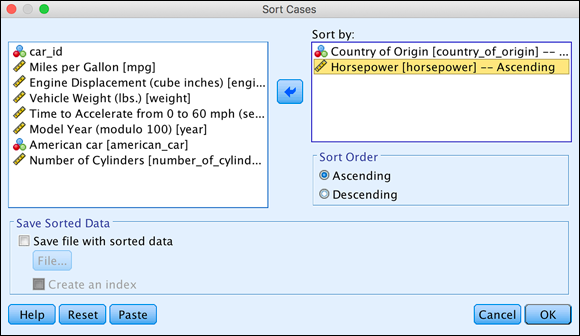
FIGURE 8-2: The Sort Cases dialog.

FIGURE 8-3: The data sorted alphabetically by country of origin and then by horsepower.
The order in which data is displayed never affects the analysis. You sort data only to better see information in Data Editor. You can get a quick sense of what’s going on by sorting your data, but in the end, it isn’t a substitute for a proper analysis in the output window.
Also, note that in the top row of data, year has a value of 0, which has been declared as a code for user-defined missing values, and the country_of_origin, american_car, and number_of_cylinders variables have system missing data. System missing values will be sorted to appear before all other values when performing a sort in ascending order. You encounter some functions for handling missing data in Chapter 10.
 If you need to sort using only one variable, you can just right-click the column name.
Selecting the Data You Want to Look At
A powerful way of manipulating your data is to turn some data off. The select cases transformation allows you to select a group and then run your analyses on only that group. In the following example, you analyze just European cars, without having to delete any data. SPSS even makes it easy to keep track of what's being counted, averaged, analyzed, and so on, and what’s turned off.
Follow these steps:
-
Choose File ⇒ Open ⇒ Data and open the Cars.sav file.
If Cars.sav is already open, that’s fine.
To make sure you see the following screenshots in the same way, you'll first sort the data on the
car_idvariable (which is how the original data file was sorted). - Choose Data ⇒ Sort Cases.
-
Choose the
car_idvariable, and then click OK to sort the data.Now that the data has been sorted on
car_id, you can select the European cars so you can do your analyses just on them. -
Choose Data ⇒ Select Cases.
The Select Cases dialog appears, as shown in Figure 8-4.
-
Select the If Condition Is Satisfied radio button and then click the If button.
Now you can specify the selection criteria.
-
Move the country_of_origin variable from the list on the left to the expression box (on the top left).
You can move the variable by either dragging it or by selecting it and then clicking the arrow button.

FIGURE 8-4: The Select Cases dialog.
-
Use your keyboard or the onscreen keypad to enter =2 in the expression box, as shown in Figure 8-5.
You have just told SPSS that you want to select only cases that have a value of 2 for the
country_of_originvariable. You type 2, and not the word European, because the stored value is 2 even though the label for a value of 2 is European. From this point forward, every piece of output that you generate will use only European cars. To return to using all cases, select the All Cases radio button in the main Select Cases dialog (refer to Figure 8-4).
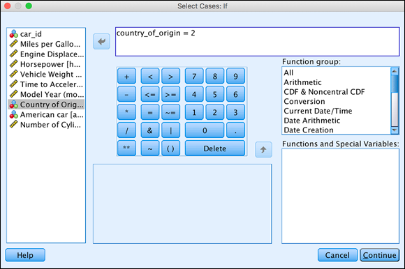
FIGURE 8-5: The If dialog.
-
Click Continue, and then click OK.
Figure 8-6 shows the final result. The slashes over some row IDs (in the first column) indicate that non-European cars are being ignored (for the time being) and only European cars are being analyzed. The
filter_$variable is also created and is comprised of 0 and 1 for Not Selected cases and Selected cases, respectively.
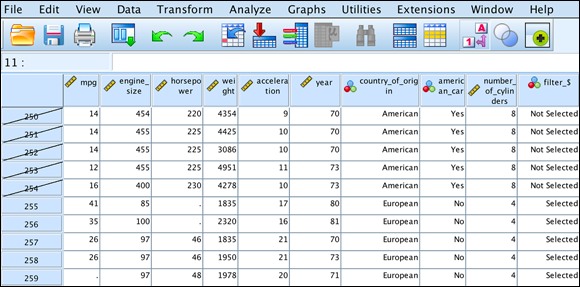
FIGURE 8-6: The data sorted, indicating selected and unselected cases.
You should always use values and labels for your category values, as we did with the country_of_origin variable in this dataset. This is the way SPSS likes it, and you don't want to make SPSS grumpy, do you? Try typing just strings, and you’re likely to get some errors and random happenings. SPSS’s bad mood could soon become your own. Use values and labels to keep everyone happy.
If you want to select complete data on a variable such as horsepower, you can use the following phrase in the Select Cases IF dialog expression box, shown in Figure 8-5: not(missing(horsepower)).
 Sometimes values such as 1, 2, and 3 appear in the data view of Data Editor, and other times labels such as American, European, and Japanese appear. In Figure 8-6 the information for
 country_of_origin currently appears as labels. To easily switch between displaying values and labels, click the value labels icon in the data window.
Splitting Data for Easier Analysis
Under some conditions, you can use an even more powerful version of what we've just illustrated with the select cases transformation. For instance, sometimes you might want to run a series of analyses on one group of cases, and then select another group of cases and rerun the same analyses on them. The split file transformation allows you to select each group in turn, one at a time, and run all your analyses on each separate group.
-
Choose File ⇒ Open ⇒ Data and open the Cars.sav file.
If Cars.sav is already open, that’s fine, but you’ll be starting with the data sorted on
car_id. Make sure that the All Cases radio button is selected in the Select Cases dialog. -
Choose Data ⇒ Split File.
The Split File dialog appears.
- Select the Compare Groups radio button.
-
Choose
country_of_originas the Compare Groups variable (see Figure 8-7) and click OK.Your data window won't have slashes as it did with the Select Cases If filter in the preceding example. Until you run some output, it won’t be clear that anything has changed.

FIGURE 8-7: The completed Split File dialog.
- Choose Analyze ⇒ Descriptive Statistics ⇒ Frequencies.
- Choose Number of Cylinders and place it in the Variable(s) box.
-
Click OK.
The resulting output, shown in Figure 8-8, is broken down by country of origin. You can stay in split mode as long as you like. Some people spend hours in split mode when producing tables, charts, and statistics for each group.

FIGURE 8-8: The frequency of number of cylinders while in split mode.
When you’re finished with the split files (or select cases) transformation, turn it off. To turn off a split, choose the Analyze All Cases, Do Not Produce Groups radio button in the Split File dialog (refer to Figure 8-7).
![]() An indicator in the bottom-right corner of the Data Editor window tells you whether a split or select operation is turned on.
An indicator in the bottom-right corner of the Data Editor window tells you whether a split or select operation is turned on.
Counting Case Occurrences
If your data is being used to keep track of multiple similar occurrences, such as people who subscribe to any combination of three different magazines, you can generate a count of the occurrences for each case. You specify what value(s) cause a variable to qualify, and SPSS creates a new variable and counts the number of qualifying variables from among those you choose. For example, if you have a number of expenses for each case, you could have SPSS count the number of expenses that exceed a certain threshold.
In the following example, people are listed as subscribers or nonsubscribers to three magazines, which are named simply mag1, mag2, and mag3. The following steps generate a total of the number of subscriptions for each person:
-
Choose File ⇒ Open ⇒ Data and open the magazines.sav file.
This file can be downloaded from the book's companion website at
www.dummies.com/go/spss. The data is shown in Figure 8-9.
FIGURE 8-9: Each magazine has the value 1 for a subscriber and 0 for a nonsubscriber.
- Choose Transform ⇒ Count Values Within Cases.
-
Do the following for each variable you want to use in the count:
- Select the variable.
- Click the arrow to move it to the Numeric Variables box.
- In the Target Variable box, give your new variable a name.
When you've finished, the screen will look like Figure 8-10. This operation works only with numerics because it must perform numeric matches on the values. If you want, you can assign both a name and a label to the variable that this process creates. In this example, the variable's name is
countand the label isCount of subscriptions.
FIGURE 8-10: The chosen variables to be counted, and the name of the new variable.
-
Click the Define Values button.
The screen shown in Figure 8-11 appears. Next, you will count the number of selected variables that have a numeric value of 1, which signifies a subscription.
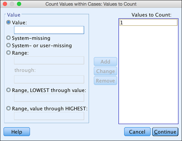
FIGURE 8-11: Define the criteria that determine which values are included in the count.
-
In the Value area, type 1 and then click the Add button to move it to the Values to Count box on the right.
After adding the value, you'll have the result shown in Figure 8-11. The new variable contains a count of the variables you named that have a value that matches at least one of the criteria you specified. Each case is counted separately.
As you can also see in figure, the total can also be based on missing values and ranges of values. In the ranges, you can specify both the high and low values, or you can specify one end of the range and have the other end be either the largest or smallest value in the set. In fact, you can select a number of criteria, and SPSS will check each variable against all of them.
-
Click Continue.
You return to the Count Occurrences of Values within Cases screen (refer to Figure 8-10).
-
Click the OK button.
Values appear for the new variable,
count, as shown in Figure 8-12.
The count transformation is a great way to assess missing data. You can count missing values across all your variables.
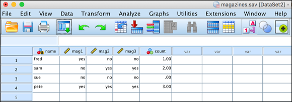
FIGURE 8-12: A new variable containing the total number of subscriptions per case.
Recoding Variables
You can have SPSS change specific values to other specific values according to rules you provide. You can change almost any value to anything else. For example, if you have Yes and No represented by 5 and 6, you could recode the values into 1 and 2, respectively. SPSS has two options for recoding variables:
- Recode into Same Variables: Recodes the values in place without creating a new variable
- Recode into Different Variables: Creates a new variable and keeps the original variable
You may want to recode to correct errors or to make the data easier to use.
If you want to recode values without creating a new variable to receive the new numbers, be sure to create a copy of your data before you start so that you don't accidently lose your data. Chapter 3 has an example of Recode into Same Variables.
Changes to your data can’t be automatically reversed, so you could destroy information. For this reason, don't use the Recode into Same Variables option unless you’re sure that you want to use it. The main reason to use this option is when you want to change a bunch of variables all at once. It's safer to stick with Recode into Different Variables.
Recoding into different variables
In this section, you use a tiny dataset so that you can see how recoding works. In the dataset, some No responses have been coded 0 and others have been coded -1. You want all No responses to be 0. Duplicate or conflicting values are common in real-world projects when data comes from multiple sources (perhaps different departments) or you have an old system and a new system.
Often you don't want to overwrite existing values — at least not at first. Instead, you want both the old and new versions of the data available. This is always a safe way to recode. You can always delete the original later if you don’t need it.
The following steps create the recoded values and stores them in a new variable:
-
Load the rsvp.sav dataset, as shown in Figure 8-13, and choose Transform ⇒ Recode into Different Variables.
This file can be downloaded from the book’s companion website at
www.dummies.com/go/spss. The Recode into Different Variables dialog appears.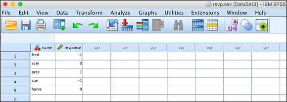
FIGURE 8-13: The rsvp.sav data file.
- In the left panel, move the
responsevariable, which holds the values you want to change, to the center panel. -
In the Output Variable area, enter a name (
attending) and label (Attending or not) for the new variable. For the output variable, if you choose a new variable name, a new variable is created. If you choose an existing variable name, its values will be overwritten. Here, you chose a new name to protect the existing data. -
Click the Change button.
The output variable is defined, as shown in Figure 8-14.
- Click the Old and New Values button.
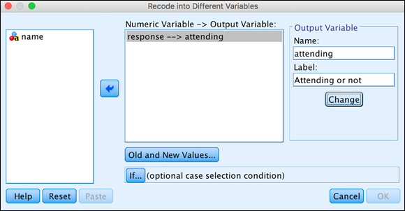
FIGURE 8-14: Name the variable to receive the recoded values.
- Define the recoding:
- In the Old Value text box, enter an existing value.
- In the New Value text box, enter the new recoded value.
-
Click the Add button for the Old ⇒ New list (see Figure 8-15).
Be sure to map all values — even the ones that don't change — because you’re creating a new variable and it has no preset values.
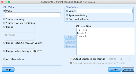
FIGURE 8-15: All possible values recoded for a new variable.
- Click Continue.
-
Click OK.
The results shown in Figure 8-16 appear. You now have a new variable and the values have been coded in a more useful manner.
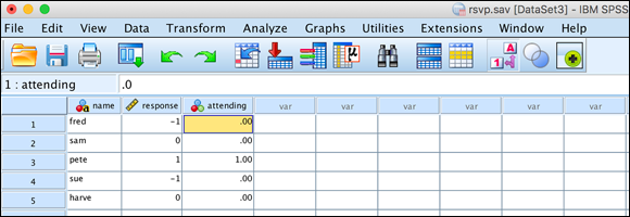
FIGURE 8-16: Values recoded into a new variable.
Automatic recoding
Automatic recoding converts string values into numeric values with labels. String variables can sometimes create confusing behaviors in SPSS because some dialogs, such as One-Way ANOVA, don’t recognize string variables, even though these dialogs do accept categorical variables.
In the following example, you work with the Embarked variable, which contains letters that represent where passengers got on the Titantic, and convert these string values into numeric values. First, however, you take a brief look at the One-Way ANOVA dialog so you can see an example of when a dialog does not display string variables. We won’t discuss the theory behind ANOVA or perform the analysis now — you learn about this statistical technique in Chapter 20.
Follow these steps:
-
Load titanic.sav.
This file can be downloaded from the book’s companion website at
www.dummies.com/go/spss. The titanic.sav dataset has become famous in machine-learning demonstrations in recent years. It contains a partial list of the passengers on the Titanic at the time of the infamous accident, when it hit an iceberg during its maiden voyage. -
Choose Analyze ⇒ Compare Means ⇒ One-Way ANOVA.
Figure 8-17 shows the One-Way Anova dialog with the Titantic.sav dataset in the background. As you can see, the dataset has 13 variables but only 8 appear in the One-Way ANOVA dialog. The 5 variables missing from the dialog are all string variables, and we would like to use one of them, the
Embarkedvariable, in a One-Way ANOVA. However, note that the previously recoded numeric variable,Embarked_Code, is visible in the One-Way ANOVA dialog. This is because this dialog does not allow string variables, even if a variable is suitable for this technique.This issue is not common, but it can be confusing when it happens. You won't pursue this analysis now. Instead, you will turn your attention to learning how to quickly and easily convert a string variable to a numeric variable with labels so that you can use the new numeric variable in practically every dialog in SPSS.

FIGURE 8-17: ANOVA dialog with a dataset in the background.
- Click Cancel to exit the One-Way ANOVA dialog.
-
Choose Transform ⇒ Automatic Recode.
The Automatic Recode dialog appears.
-
In the list on the left, move the variable you want to recode to the box on the left.
To follow along with the example, move the
Embarkedvariable. -
In the Variable ⇒ New Name box, enter the name of the variable to receive the recoded values.
Type the name
Embarked_Code2. -
Click the Add New Name button.
Embarked_Code2appears in the box above the new name. - Select the Treat Blank String Values as User-Missing option, as shown in Figure 8-18.

FIGURE 8-18: The dialog for automatic recoding.
-
Click OK.
Recoding takes place, as shown in the output window shown in Figure 8-19. The M adjacent to the value 4 indicates that not only have the missing values been assigned to the numeric value 4 but SPSS also has declared value 4 as missing.

FIGURE 8-19: Autorecoded values.
The values in the new variable, Embarked_Code2, come about from sorting the values of the original variable and then assigning numbers to them in the new sort order. If the input values are a string of characters instead of the digits, the strings are sorted alphabetically (well, almost — uppercase letters come before lowercase).
In the Automatic Recode window (refer to Figure 8-18), you can see the choice for recoding values with new numbers that start with either the lowest value or the highest value. The new numeric values will be the same either way; they're just assigned in the opposite order.
At the bottom of the Automatic Recode window are two choices for the creation of a template file. A template file holds a record of the recoding patterns. That way, if you want to recode more data with the same variable names, the new input values will be compared against the previous encoding and be given appropriate values so that the two data files can be merged and the data will all fit. For example, if you have brand names or part numbers in your data, the recoding will be consistent with the original values because it will be assigned the same pattern of recoded values.
Binning
If you’re using a scale variable, which contains a range of values, you can create groups of those values and organize them in bins. For example, you could use the ages of a number of people and put each one in its own bin, such as one bin for ages 0 to 20, another bin for ages 21 to 40, and so on. You can specify the size and content of bins in several ways. The actual binning process is automatic.
The following steps divide salaries into bins:
-
Choose File ⇒ Open ⇒ Data and load the salaries.sav file.
To download the file, go to
www.dummies.com/go/spss4e. The file contains a list of ID numbers with a salary for each one, as shown in Figure 8-20.
FIGURE 8-20: A list of employee ID numbers and the salaries corresponding to them.
-
Choose Transform ⇒ Visual Binning.
The Visual Binning dialog appears.
- Move
Current Salaryfrom the Variables box to the Variables to Bin box, as shown in Figure 8-21.
FIGURE 8-21: Select the name of the variable to be binned.
-
Click Continue.
A bar graph displaying the range of values of the salaries appears, as shown in Figure 8-22.

FIGURE 8-22: How the binning will be done.
- Click the Make Cutpoints button.
-
Select the points at which you want to cut the data into parts to create the bins.
In this example, we divided the data into even percentiles of numbers of cases — that is, each bin will contain the same number of cases, as shown in Figure 8-23. Note that four cutpoints divide the data into five bins, each holding 20 percent of the cases.
We could have divided the data into equal-width intervals — that is, each bin would contain a range of the same magnitude, which would put different numbers of cases in each bin. Or the cutpoints could have been based on standard deviations, which would create two cutpoints, dividing the data into the three bins — one each of low, medium, and high capacity.

FIGURE 8-23: Specify how you want the data divided into bins.
-
Click the Apply button, and the cutpoints appear as vertical lines on the bar graph, as shown in Figure 8-24.
You can click the Make Cutpoints button repeatedly and cut the data different ways until you get the cutpoints the way you like. Any new cutpoints you define replace previous ones.
-
In the Binned Variable text box, enter salary_bin as the new variable to contain the binning information.
Be sure to use an underscore. The default label for the new variable appears in the text box to the right of the name. You can change this if you want.
The bins are created and numbered from 1 to 5, but if you select the Reverse Scale option (in the lower-right corner), the numbering will be from 5 to 1.

FIGURE 8-24: A bar graph of the data with cutpoints for binning.
-
Click OK.
The message in Figure 8-25 appears. Don't worry. Nothing is wrong because you want to create a new variable.

FIGURE 8-25: A message alerting that you are about to create a new variable.
-
Click OK to dismiss the warning message.
The new variable is created and filled with the bin values, as shown in Figure 8-26.
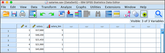
FIGURE 8-26: The new variable containing the bin numbers.
Optimal Binning
Another kind of binning called optimal binning is easy but powerful, using technology similar to that used in machine learning. Optimal binning finds the cutpoints that are optimal for predictions.
Follow these steps to perform optimal binning:
- Return to the titanic.sav dataset. Choose Transform ⇒ Optimal Binning.
-
Move the
Farevariable to the Variables to Bin box, and moveSurvivedto the Optimize Bins with Respect To box, as shown in Figure 8-27.The variable in the Optimize Bins with Respect To box doesn’t have to be a variable from a previous binning operation. It can be any variable that contains a collection of values that can be separated into bins.
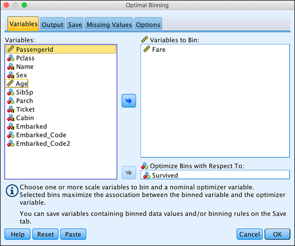
FIGURE 8-27: Select the bin variable and the optimizing variable.
-
Click OK.
The output shown in Figure 8-28 is generated.

FIGURE 8-28: The output from optimal binning.
The results are interesting. The fares are in British pounds, but remember that the Titanic accident happened in 1912. The upper cutoff of 10.5 for Bin 1 (shown in Figure 8-28), adjusted for inflation, would be over 1,000 British pounds today. The survival rate for Bin 1, the lowest fares, is 67/339, or about 20 percent. The survival rate for Bin 3 is 74/97, well over 75 percent. So you've learned not just that fare is related to survival but also something specific about the optimal points along the fare continuum where you can most easily perceive changes in survival rate. Optimal binning is a powerful feature.