Chapter 15
Knowing When Not to Trust Your Data
IN THIS CHAPTER
![]() Working with samples
Working with samples
![]() Testing hypotheses
Testing hypotheses
![]() Understanding confidence intervals
Understanding confidence intervals
![]() Using the normal distribution
Using the normal distribution
![]() Calculating Z-scores
Calculating Z-scores
What is inferential statistics and who uses it? Inferential statistics is the practice of collecting and analyzing numerical data for the purpose of making scientific inferences from a representative sample to a population. Government agencies, business analysts, market researchers, health researchers, survey companies, education researchers, and many others use inference.
In this chapter, you discover the benefits and potential limitations of sampling. You then find out about hypothesis testing so you can learn the logic behind performing statistical tests. From there, we describe distributions, which provide insight into statistical theory and will lead you to calculating z-scores, so that you can identify the position of any data point on a distribution.
Sampling
Descriptive statistics, which we introduce in Chapter 14, describe the data in a sample through a number of summary procedures and statistics. For example, you can calculate the mean or standard deviation of a group of people so that you can better describe them. Descriptive statistics are mostly useful if you just want to describe a specific sample. Most of the time, however, researchers are concerned not about a sample but about a population. They use the results from a sample to make inferences about the true values in a population.
In an ideal world, you'd collect data from every single person you’re interested in. Because that is not realistic, you use samples. Sampling is the process of collecting data on a portion of all the elements of interest as an alternative to looking at the entire set of elements. Sampling allows us to describe and draw conclusions about the population, and is performed for feasibility, accessibility, and efficiency in terms of both time and money. If you follow some rules when sampling, you can get answers that are close to the population values, with high probability.
Following are the characteristics of an effective sample:
- Probabilistic sampling: One in which each element of the population has a known, nonzero chance of being included in the sample. A probability sample allows you to do statistical tests, place confidence intervals around statistics (so that you know the probable range of values), and make inferences about the total population.
- Sufficiently large: Small samples will not provide the appropriate statistical power to discover true differences between groups or to determine the effect of one variable on another.
- Unbiased: Bias occurs because some units are overselected or underselected for the sample. Some types of bias include selection bias in how the sampling itself is done, and nonresponse bias, which occurs when those who decline to participate are different than those who do respond.
 With nonprobability samples (such as snowball, convenience, quota, or focus groups), calculating the probability of selection for all elements in the population is impossible. Therefore, statistical theory does not apply to a nonprobability sample, which tells us only about the elements in the sample, not about any greater population.
Understanding Sample Size
An important aspect of statistics is that they vary from one sample to another. Due to the effects of random variability, it is unlikely that any two samples drawn from the same population will produce the same statistics.
By plotting the values of a particular statistic, such as the mean, from a large number of samples, you can obtain a sampling distribution of the statistic. For small numbers of samples, the mean of the sampling distribution may not closely resemble that of the population. However, as the number of samples taken increases, the closer the mean of the sampling distribution (the mean of all the means) gets to the population mean. For an infinitely large number of samples, the mean will be exactly the same as the population mean.
Additionally, as sample size increases, the amount of variability in the distribution of sample means decreases. If you think of variability in terms of the error made in estimating the mean, it should be clear that the more evidence you have — that is, the more cases in the sample — the smaller the error in estimating the mean.
Sample size strongly influences precision, that is, how close estimates from different samples are to each other. As an example, the precision of a sample proportion is approximately equal to one divided by the square root of the sample size. Table 15-1 displays the precision for various sample sizes.
TABLE 15-1 Sample Size and Precision
|
Sample Size |
Precision |
|
100 |
1/√100 = 10% |
|
400 |
1/√400 = 5% |
|
1,600 |
1/√1600 = 2.5% |
Testing Hypotheses
Suppose you collected customer satisfaction data on a subset of your customers and determine that the average customer satisfaction is 3.5 on a 5-point scale. You want to take this information a step further, though, and determine whether a difference in satisfaction exists between customers who bought Product A (3.6) and customers who bought Product B (3.3). The numbers aren’t exactly the same, but are the differences due to random variation? Inferential statistics can answer this type of question.
Inferential statistics enables you to infer the results from the sample on which you have data and apply it to the population that the sample represents. Understanding how to make inferences from a sample to a population is the basis of inferential statistics. You can reach conclusions about the population without studying every single individual, which can be costly and time consuming.
Whenever you want to make an inference about a population from a sample, you must test a specific hypothesis. Typically, you state two hypotheses:
- Null hypothesis: The null hypothesis is the one in which no effect is present. For example, you may be looking for differences in mean income between males and females, but the (null) hypothesis you’re testing is that there is no difference between the groups. Or the null hypothesis may be that there are no differences in satisfaction between customers who bought Product A (3.6) and customers who bought Product B (3.3). In other words, the differences are due to random variation.
- Alternative hypothesis: The alternative hypothesis (also known as the research hypothesis) is generally (although not exclusively) the one researchers are really interested in. For example, you may hypothesize that the mean incomes of males and females are different. Or for the customer satisfaction example, the alternative hypothesis may be that there is a difference in satisfaction between customers who bought Product A (3.6) and customers who bought Product B (3.3). In other words, the differences are real.
When making an inference, you never know anything for certain because you’re dealing with samples rather than populations. Therefore, you always have to work with probabilities. You assess a hypothesis by calculating the probability, or the likelihood, of finding your result. A probability value can range from 0 to 1 (corresponding to 0 percent to 100 percent, in terms of percentages). You can use these values to assess whether the likelihood that any differences you’ve found are the result of random chance.
So, how do hypotheses and probabilities interact? Suppose you want to know who will win the Super Bowl. You ask your fellow statisticians, and one of them says that he has built a predictive model and he knows Team A will win. Your next question should be, “How confident are you in your prediction?” Your friend says, “I’m 50 percent confident.” Are you going to trust this prediction? Of course not, because there are only two outcomes and 50 percent means the prediction is random.
So, you ask another fellow statistician, and he tells you that he has built a predictive model. He knows that Team A will win, and he’s 75 percent confident in his prediction. Are you going to trust his prediction? Well, now you start to think about it a little. You have a 75 percent chance of being right and a 25 percent chance of being wrong, and decide that a 25 percent chance of being wrong is too high.
So, you ask another fellow statistician, and she tells you that she has built a predictive model and knows Team A will win, and she’s 90 percent confident in her prediction. Are you going to trust her prediction? Now you have a 90 percent chance of being right, and only a 10 percent chance of being wrong.
This is the way statistics work. You have two hypotheses — the null hypothesis and the alternative hypothesis — and you want to be sure of your conclusions. So, having formally stated the hypotheses, you must then select a criterion for acceptance or rejection of the null hypothesis. With probability tests, such as the chi-square test of independence or the independent samples t-test, you’re testing the likelihood that a statistic of the magnitude obtained (or greater) would have occurred by chance, assuming that the null hypothesis is true.
Remember, you always assess the null hypothesis, which is the hypothesis that states there is no difference or no relationship. In other words, you reject the null hypothesis only when you can say that the result would have been extremely unlikely under the conditions set by the null hypothesis; if this is the case, the alternative hypothesis should be accepted.
 But what criterion (or alpha level, as it is often known) should you use? Traditionally, a 5 percent level is chosen, indicating that a statistic of the size obtained would be likely to occur on only 5 percent of occasions (or once in 20 occasions) should the null hypothesis be true. By choosing a 5 percent criterion, you’re accepting that you’ll make a mistake in rejecting the null hypothesis 5 percent of the time (should the null hypothesis be true).
 Hypothesis testing has been frustrating students and instructors of statistics for years! Don’t be surprised if you have to reread this chapter several times — hypothesis testing is confusing stuff!
Calculating Confidence Intervals
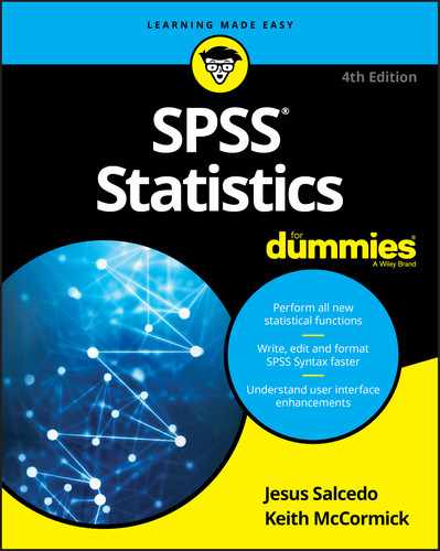
Consider the example in Figure 15-1, in which a treatment group has a mean of 14.43 and a control group has a mean of 12.37. You need to detect whether the means are significantly different or due to chance.
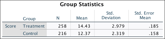
FIGURE 15-1: The Group Statistics table.
A 95 percent confidence interval provides a measure of the precision with which the true population difference is estimated. In the example (see Figure 15-2), the 95 percent confidence interval for the mean difference between groups ranges from 1.571 to 2.549; the actual mean difference is 2.06. So the 95 percent confidence interval indicates the likely range of the population mean difference.
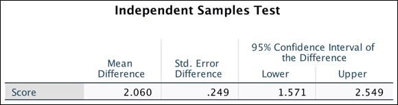
FIGURE 15-2: The Independent Samples test.
Although the actual value is 2.06, you are 95 percent confident that the difference value will fall anywhere between 1.571 to 2.549 (basically the mean difference +/- the standard error of the difference (.249) multiplied by 1.96).
The only value that you're getting directly from the data is the mean, 2.06. Statistics students often memorize the number 1.96, which is the 5 percent cutoff from the normal distribution — but not from this specific dataset. So the lower value (1.571) and upper value (2.549) of the confidence interval are derived using the value 1.96, which assumes a normal distribution. If the distribution is not normal, the confidence interval numbers will be wrong.
Note that the confidence interval does not include zero because there is a statistically significant difference between groups. If zero had been included within the range, it would indicate that there are no differences between the groups — that is, you’re saying that the probability value is greater than 0.05. In essence, the 95 percent confidence interval is another way of testing the null hypothesis. So, if the value of zero does not fall within the 95 percent confidence interval, you’re saying that the probability of the null hypothesis (that is, no difference or a difference of zero) is less than 0.05.
Conducting In-Depth Hypothesis Testing
We just introduced inferential statistics, which allows us to infer the results from your sample to the population. This concept is important because you want to do research that applies to a larger audience than just the specific group of people you test.
As mentioned, hypothesis testing allows researchers to develop hypotheses, which are then assessed to determine the probability, or likelihood, of the findings. Two hypotheses are typically created: The null hypothesis states that no effect is present, and the alternative hypothesis states that an effect is present.
For example, suppose you want to assess whether differences in mean income exist between males and females. The null hypothesis states that there is no difference in income between the groups, and the alternative hypothesis states that there is a difference in income between the groups. You then assess the null hypothesis by calculating the probability that it is true. At this point, you investigate the probability value, and if it’s less than 0.05, you say that you’ve found support for the alternative hypothesis because the probability that the null hypothesis is true is low (less than 5 percent). If it’s greater than 0.05, you say that you've found support for the null hypothesis because there is a decent chance that it’s true (greater than 5 percent).
However, too often people immediately jump to the conclusion that the finding is statistically significant or is not statistically significant. Although that’s literally true, because you use those words to describe probability values below 0.05 and above 0.05, statistical significance doesn’t imply that only two conclusions can be drawn about your finding. Table 15-2 is a more realistic scenario.
TABLE 15-2 Types of Statistical Outcome
|
In the Real World |
Statistical Test Outcome |
|
Not Significant |
Significant |
|
|
No difference (null is true) |
Correct decision |
False positive; Type I error |
|||
|
True difference (alternative is true) |
False negative; Type II error |
Correct decision, power |
|||
Note that several outcomes are possible. Let’s take a look at the first row. It could be that, in the real world, there is no relationship between the variables, which is what your test found. In this scenario, you would be making a correct decision. However, what if in the real world there was no relationship between the variables and your test found that there was a significant relationship? In this case, you would be making a Type 1 error. This type of error is known also as a false positive because the researcher falsely concludes a positive result (thinks it does occur when it does not).
A Type I error is explicitly taken into account when performing statistical tests. When testing for statistical significance using a 0.05 criterion, you acknowledge that if there is no effect in the population, the sample statistic will exceed the criterion on average 5 times out of 100 (or 0.05). So this type of error could occur strictly by chance — or if the researcher used the wrong test. (An inappropriate test is used when you don’t meet the assumptions of a test, which is why knowing and testing assumptions is important.)
How could SPSS let you do the wrong test? The calculations will always be correct, but you have to know which menu to work in. For instance, the T-test is a parametric test, and it assumes that your data is shaped like a bell curve. In fact (and this is even more technical), it assumes that the errors are shaped like a bell curve. And there is a separate menu with tests that you can use when this isn’t true. You may be surprised by how many SPSS users get confused about these issues. What happens is this: A parametric test might yield a probability of 0.047 and a nonparametric test might yield a probability of 0.053. You can see the problem now. If you declare a result is significant, an expert might say the same result is not significant.
 For now, the main message is this — assumptions are not just a bunch of arbitrary rules. They sometimes affect which conclusions you draw.
Now let’s take a look at the second row of Table 15-2. It could be that in the real world there is a relationship between the variables, and this is what your test found. In this scenario, you would be making a correct decision. Power is defined as the ability to detect true differences if they exist.
However, what if in the real world there was a relationship between the variables and your test found that there was no significant relationship? In this case, you would be making a Type II error. This type of error is known also as a false negative because the researcher falsely concludes a negative result (thinks it does not occur when in fact it does). This type of error typically happens when you use small samples, so your test is not powerful enough to detect true differences. (When sample sizes are small, precision tends to be poor.) The error could occur also if the researcher used the wrong test.
You know that larger samples are more precise, thus power analysis was developed to help researchers determine the minimum sample size required to have a specified chance of detecting a true difference or relationship.
Power analysis can be useful when planning a study but you must know the magnitude of the hypothesized effect and an estimate of the variance.
A related issue involves drawing a distinction between statistical significance and practical importance. When an effect is found to be statistically significant, you conclude that the population effect (difference or relation) is not zero. However, this conclusion allows for a statistically significant effect that is not quite zero yet so small as to be insignificant from a practical or policy perspective.
As mentioned, very large samples yield increased precision, and in such samples very small effects may be found to be statistically significant but the question is whether the effects make any practical difference. For example, suppose a company is interested in customer ratings of one of its products and obtains scores from several thousand customers. Furthermore, suppose the mean ratings on a 1 to 5 satisfaction scale are 3.25 for male customers and 3.15 for female customers, and this difference is found to be statistically significant. Would such a small difference be of any practical interest or use?
When sample sizes are small (say under 30), precision tends to be poor and so only relatively large effects are found to be statistically significant. With moderate samples (say 50 to 200), small effects tend to show modest significance while large effects are highly significant. For very large samples (several hundred or thousand), small effects can be highly significant. Thus, an important aspect of an analysis is to examine the effect size and determine if it is important from a practical or policy perspective.
Using the Normal Distribution
The distribution of a variable refers to the numbers of times each outcome occurs. Many statistical distributions exists, such as binomial, uniform, and Poisson, but one of the most common distributions is the normal distribution. Many naturally occurring phenomena, such as height, weight, and blood pressure, follow a normal distribution (curve).
The normal distribution (often referred to as the normal bell-shaped curve) is a frequency distribution in which the mean, median, and mode exactly coincide and are symmetrical, so that 50 percent of cases lie to either side of the mean. In addition, the proportion of cases contained within any portion of the normal curve can be calculated mathematically, which is why the normal distribution is used in many inferential statistical procedures. Figure 15-3 illustrates a normal distribution.
Random errors tend to conform to a normal distribution, which is why many statistical techniques have the assumption of normality, which says that errors follow a normal distribution. In fact, every statistical technique that we describe that has a continuous dependent variable has the assumption of normality. In Chapter 21, we talk about situations and tests you can use when you don't have a normal distribution.
FIGURE 15-3: A normal distribution.
Normal distributions are frequently used in statistics also because the Central Limit Theorem suggests that as sample size increases, the sampling distribution of the sample's means approaches normality, regardless of the shape of the population distribution. This extremely useful statistical axiom doesn't require that the original population distribution be normal; it states that the sample mean is distributed normally, regardless of the distribution of the variable itself.
Working with Z-Scores
After you know the characteristics of the distribution of a variable, that is, the mean and standard deviation, you can calculate standardized scores, more commonly referred to as z-scores. Z-scores indicate the number of standard deviations a score is above or below the sample mean. You can use standardized scores to calculate the relative position of each value in a normal distribution because the mean of a standardized distribution is 0 and the standard deviation is 1. Z-scores are most often used in statistics to standardize variables of unequal scale units for statistical comparisons or for use in multivariate procedures.
Z-scores are calculated by subtracting the mean from the value of the observation in question and then dividing by the standard deviation for the sample:
Z = (score - mean) / standard deviation
For example, if you have a score of 75 out of 100 on a test of math ability, this information alone is not enough to tell how well you did in relation to others taking the test. However, if you know that the mean score and the standard deviation, you can calculate the proportion of people who achieved a score at least as high as you. For example, if the mean is 50 and the standard deviation is 10, you can calculate the following:
(75 - 50) / 10 = 2.5
You scored 2.5 standard deviations above the mean.
In Chapter 14, we show you how to use the descriptives procedure as an alternative to the frequencies procedure. Now you use the descriptives procedure to calculate z-scores.
To use the descriptives procedure, follow these steps:
-
From the main menu, choose File ⇒ Open ⇒ Data, and load the Merchandise.sav data file.
The file is not in the SPSS installation directory. Download it from the book’s companion website at
www.dummies.com/go/spss4e. - Choose Analyze ⇒ Descriptive Statistics ⇒ Descriptives.
- Select the Stereos, TVs, and Speakers variables and place them in the Variable(s) box.
- Select the Save Standardized Values as Variables option, as shown in Figure 15-4.

FIGURE 15-4: The Descriptives dialog used to calculate z-scores.
-
Click OK.
SPSS runs the descriptives procedure and calculates the z-scores.
- Switch over to the Data Editor window.
Figure 15-5 shows the three new standardized variables created at the end of the data file. Note that the screen was split to better illustrate the creation of the new variables. By default, the new variable names are the old variable names prefixed with the letter Z. You can save these variables in the file and use them in any statistical procedure.

FIGURE 15-5: The Stereos, TVs, and Speakers variables have been standardized.
Focusing on the first row, note that the first person purchased 5 stereos, 8 TVs, and 86 speakers. Typically, you'd think that 86 is a large number, but when you look at the z-scores, the only value above average is for the number of TVs purchased, not stereos purchased. Figure 15-6 shows the respective mean and standard deviation for each variable. Given that the mean number of TVs purchased is .83 with a standard deviation of 2.23, someone buying 8 TVs is unusual.
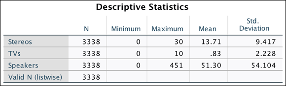
FIGURE 15-6: The Descriptive Statistics table of stereos, TVs, and speakers.