Chapter 10
Some Useful Functions
IN THIS CHAPTER
![]() Learning the language of SPSS functions
Learning the language of SPSS functions
![]() Using the
Using the LENGTH function
![]() Working with the
Working with the ANY function
![]() Making the
Making the MEAN function work for you
![]() Expanding your toolkit of functions
Expanding your toolkit of functions
In this chapter, we focus on the variety of functions available in the Compute Variable dialog. We won't discuss them all, but we do provide examples of several of the most useful ones. If you use spreadsheet software such as Microsoft Excel or Apple Numbers, you've encountered some of these functions, but SPSS offers a greater variety of statistical options than you’ll find in spreadsheet software. We emphasize the functions aligned with the most important SPSS skills.
SPSS divides functions into function groups. Here’s just a sampling of the kinds of functions you’ll find:
- Arithmetic functions
- Statistical functions
- String functions
- String/numeric conversion functions
- Date and time functions
- Random variable and distribution functions
- Missing value functions
- Logical functions
When you click a function group name such as Arithmetic (refer to Figure 10-1), you see a list of the functions that belong to that function group. In this chapter, you investigate just 12 of these functions, but they're a diverse 12. The idea is to give you a sense of the different kinds of things you can do and to introduce you to the function help system.

FIGURE 10-1: The Compute Variable dialog with the Arithmetic function group selected.
The LENGTH Function
For the initial examples, you use the Web Survey.sav dataset. The end of the Web Survey.sav dataset has an open-ended question where respondents can leave a comment. This type of question often prompts a generic answer such as “Not at this time” or “None,” but sometimes the responses can be useful.
The goal of this exercise is to identify, as simply as possible, if the respondent provided a comment. That way, you won’t clog up your report with lots of blank rows. To do so, you use the LENGTH function.
The LENGTH function identifies the number of characters in a response, so anyone with a value greater than zero provided a response. This function also allows you to review some features of the help that SPSS provides for each function. This simple function is a good place to start because it requires only one argument:
-
Open the Web Survey.sav dataset.
To download the file, go to the book's companion website at
www.dummies.com/go/spss4e. (You may stumble upon Web Survey 2.sav, which is what the dataset looks like at the end of the chapter.) - Choose Transform ⇒ Compute Variable.
- Select String in the Function Group area in the upper right, and then select the
Lengthfunction. -
Either drag
Lengthinto position in the editing area at the top, or click the up-arrow button on the right.The window should look like Figure 10-2.

FIGURE 10-2: The Compute Variable dialog with the
LENGTHfunction selected. -
Select the
Commentvariable and either drag it into position, replacing the question mark, or click the right-arrow button on the left.Making progress. You could just click OK, but let's take a moment to read the function help at the bottom of the screen, which is visible whenever you click a function's name (as you did for
Lengthin Figure 10-2). You have to scroll to read it onscreen; the complete text is as follows:LENGTH(strexpr). Numeric. Returns the length of strexpr in bytes, which must be a string expression. For string variables, in Unicode mode this is the number of bytes in each value, excluding trailing blanks, but in code page mode this is the defined variable length, including trailing blanks. To get the length (in bytes) without trailing blanks in code page mode, use LENGTH(RTRIM(strexpr)).
Whoa! This information can be intimidating at first, but it is all there for a reason. The function help section has the following consistent structure across all functions in SPSS:
- Function name and grammar
- Type of output
- Description of the function
The first part — LENGTH(strexpr) — is the name and grammar of the function. You have to give the command a string expression in parentheses. Next, the word Numeric means that the function will return a numeric value. This pattern is repeated for every function. The first two parts are half the battle! The final part, which isn’t always easy to read, is the description of how the function works.
In this case, you give the
LENGTHfunction a word, and it gives you a number. Let's try it. - In the Target Variable box, name the new variable Length and verify that your screen looks like Figure 10-3.

FIGURE 10-3: The completed
LENGTHfunction in the Compute Variable dialog. -
Click OK.
In the data window, you see a new variable,
Length, listing several numbers. Glance at the originalCommentvariable. Doug, Jack, and Georgia did not leave comments, so they should have a zero value.
The ANY Function
Learning the grammar of a function includes identifying the number of required arguments or components. The LENGTH function has only one argument. Now you move on to a more complex function, the ANY function, which has two arguments.
When analyzing data, it's often useful to identify people who meet certain criteria. For example, you may want to identify employees who have high performance ratings (to keep them in mind for future job openings), or you may want to identify customers who gave your company a low satisfaction rating (to see how you can improve their experience). The ANY function allows you to identify cases that meet the criteria you specify across a series of variables.
In this example, you identify customers who gave a response of 1, the lowest possible value, on the satisfaction variables, so you can contact them and address their concerns.
- If the Web Survey.sav dataset is not still open, open it now.
- Choose Transform ⇒ Compute Variable.
- In the Function Group area in the upper right, select Search and then select the
Anyfunction. -
Either drag
Anyinto position in the editing area at the top, or click the up-arrow button on the right.The window should look like Figure 10-4.
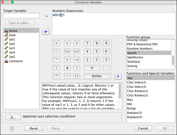
FIGURE 10-4: The Compute Variable dialog with the
ANYfunction chosen. -
Review the function definition at the bottom of the dialog.
Let's take a moment to read the function help for
ANYat the bottom of the dialog:- ANY(test,value[,value,…]). Logical. Returns 1 or true if the value of test matches any of the subsequent values; returns 0 or false otherwise. This function requires two or more arguments. For example, ANY(var1, 1, 3, 5) returns 1 if the value of var1 is 1, 3, or 5 and 0 for other values. ANY can also be used to scan a list of variables or expressions for a value. For example, ANY(1, var1, var2, var3) returns 1 if any of the three specified variables has a value of 1 and 0 if all three variables have values other than 1.
Most people find these definitions difficult at first, but remember: It all means something. The first part — ANY(test,value[,value,…]) — is the name and grammar of the function. Note that it has more arguments than
LENGTH, so it's a little more complicated. The next word — Logical — tells you that you're going to get a true or false result, which SPSS indicates with 1 and 0, respectively. Finally, the third section describes the purpose of the function. Again, the structure of the help section remains consistent.So the definition means that you give the
ANYfunction a test value and several variable names, and it will give you a 1 or a 0. Let’s try it. - In the Target Variable box, name the new variable Any_Ones.
-
In the Numeric Expression box, replace the first question mark with 1.
It looks like you have room for only one more variable because you have only one more question mark, but you can add as many as you like.
- Drag all the
Satvariables (Sat1,Sat2,Sat3,Sat4, andSat5), separating each with a comma, and replacing the second question mark, as shown in Figure 10-5. -
Click OK.
The data window displays a new variable,
Any_Ones, which is 1 (true) or 0 (false), depending on whether the respondent gave a 1 (the lowest score) for any of the satisfaction variables. You could easily imagine that management at this company wants to know if anyone is upset enough to give a score of 1 on any question.
 Before attempting to run any function, make sure you delete all question marks in the function. Otherwise, you will not be able to run the command.
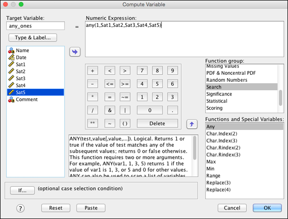
FIGURE 10-5: The dialog with the completed ANY function.
The MEAN Function and Missing Data
Next, you calculate the mean of the five satisfaction variables. There is a twist, though — you can include or exclude rows with some missing data. If the respondent didn't answer any of the questions, you don’t have much choice, but what if someone answered only some questions? Here’s how to calculate a mean in two different ways:
- If Web Survey.sav isn't open, open it.
- Choose Transform ⇒ Compute Variable.
- Select Statistical in the Function Group area, and then select the
Meanfunction. - Either drag
Meaninto position in the editing area at the top, or click the up-arrow button on the right. -
Review the function definition at the bottom of the dialog.
Here's what it says:
- MEAN. MEAN(numexpr,numexpr[,..]). Numeric. Returns the arithmetic mean of its arguments that have valid, nonmissing values. This function requires two or more arguments, which must be numeric. You can specify a minimum number of valid arguments for this function to be evaluated.
The first word is the name of the function. The second part — MEAN(numexpr,numexpr[,..]) — means you have to provide at least two variables; the two dots indicate that you can provide more than two variables, if needed. The next word — Numeric — tells you that the result will be a number. Note that you can specify a minimum number of valid arguments for this function to be evaluated. This functionality will be important in the second example.
To summarize, you give
MEANseveral variable names (or numbers), and it returns a number. - In the Target Variable box, name the new variable Mean_Sat.
- Drag all the
Satvariables (Sat1,Sat2,Sat3,Sat4, andSat5)), separating each with a comma, to the Numeric Expression box, as shown in Figure 10-6.
FIGURE 10-6: The completed
MEANfunction that allows for missing values. -
Click OK.
The Data Editor window displays the new variable,
Mean_Sat, populated for everyone, even though Frank didn't answer all the questions. His average is based on the answers he did provide. -
Choose Transform ⇒ Compute Variable.
The previous expression that you created in the Compute Variable dialog is still there.
- Name the new variable Mean_Sat2.
-
In the Numeric Expression box, add .5 to the function so that it reads
MEAN.5, as shown in Figure 10-7.Don't change the rest of the function.
The
.5(the .n suffix) tells SPSS Statistics that to compute a mean, each case must provide at least five valid values. Here you are specifying the minimum number of valid arguments for this function to be evaluated.
FIGURE 10-7: The completed
MEANfunction requiring five valid values. -
Click OK.
The Data Editor window displays the new variable,
Mean_Sat2, which is populated for everyone except Frank because he didn't answer all the questions.
This is powerful stuff. Mastering missing values is one of the things that will mark you as an expert in SPSS Statistics.
 Specifying the minimum number of valid arguments for a function to be evaluated (the .n suffix) works with all statistical functions, notably the
 SUM() function.
If you want to read extended documentation on functions, go to Command Syntax Reference in the Help menu. Make sure look in Chapter 2, “Universals,” under “Transformation Expressions.” If you look in the section for the Compute command, the information is much more limited and you might not find what you need.
RND, TRUNC, and MOD
SPSS allows you to declare and display numeric variables with up to 16 decimal places, which is far more than you will typically want to report. SPSS uses all of this precision when performing calculations, whether you display them or not. In some instances, you'll want to convert real numbers into integers.
The Arithmetic function group offers a number of options to do this kind of conversion. In this section, you explore three functions: RND (rounds to the nearest integer), TRUNC (truncates the remainder), and MOD (returns the remainder).
The loan_payment.sav dataset, available on the book's website (www.dummies.com/go/spss4e) and shown in Figure 10-8, includes information about how long it’s been since loans were originated. It’s reported in months because statements are sent out monthly. A simple calculation (dividing by 12) would calculate the number of years, but what if you wanted to report years and months?
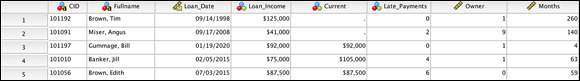
FIGURE 10-8: The loan_payment.sav dataset.
At this point, you're familiar with the Compute Variable dialog, so Table 10-1 simply shows possible alternatives to place in the expression box using the simple formula and three different functions.
Note that the MOD() function takes two arguments, so it requires a comma to separate the two arguments. The second argument, called the modulus, is 12 because the divisor is 12. As you can see, the best way to report years and months is to use the combination of the TRUNC() and MOD() functions. For instance, CID 101192 has had a loan for 21 years and 8 months.
TABLE 10-1 Arithmetic Function Results
|
CID |
Months |
Months/12 |
Rnd(Months/12) |
Trunc(Months/12) |
Mod(Months,12) |
|
101192 |
260 |
21.67 |
22 |
21 |
8 |
|
101091 |
140 |
11.67 |
12 |
11 |
8 |
|
101197 |
4 |
.33 |
0 |
0 |
4 |
|
101010 |
63 |
5.25 |
5 |
5 |
3 |
|
101056 |
59 |
4.92 |
5 |
4 |
11 |
Don't use the Variable View tab of the Data Editor window (see Chapter 3) to attempt to convert real numbers to integers. Changing the number of decimal places in the Variable View tab changes only the decimal places that appear in the Data Editor window; it doesn't change the number of decimal places stored in the variable or in any calculations. The decimal places are still there even if you can't see them. Change the decimal places back again and they will return to view.
 A number of arithmetic functions have an optional
 fuzzbits argument. The vast majority of SPSS users can safely ignore this argument. It relates to significant digits and can become an issue when making calculations and then reporting to many decimal places. When reporting at this level of precision, Excel, SAS, and SPSS can disagree due to subtle little differences in the calculations. If this ever happens, research fuzzbits in the Command Syntax Reference.
Logicals, the MISSING Function, and the NOT Function
Many SPSS functions, such as the ANY function (which you used previously), the MISSING function, and the SYSMIS function, return 1 for true and 0 for false. The 1s and 0s are not labeled, which can be confusing. Most computer programming languages call this kind of variable a Boolean, or binary, variable because it has two possible outcomes.
The MISSING function is true if a value is either user-defined missing or system missing. The SYSMIS function returns true only when the value is system missing.
The SPSS feature of user-defined missing (see Chapter 3) involves an otherwise valid value that has been declared as missing in the Variable View tab of the Data Editor window. In this dataset, the Owner variable has a user-defined missing value of 9, meaning unverified, whereas the Current variable has two system missing values. The results of four different variables created by Compute Variable when using the MISSING and SYSMIS functions are shown in Table 10-2.
TABLE 10-2 MISSING() and SYSMIS() Function Results
|
CID |
Missing(Current) |
Missing(Owner) |
Sysmis(Current) |
Sysmis(Owner) |
|
101192 |
1 |
0 |
1 |
0 |
|
101091 |
1 |
1 |
1 |
0 |
|
101197 |
0 |
0 |
0 |
0 |
|
101010 |
0 |
0 |
0 |
0 |
|
101056 |
0 |
0 |
0 |
0 |
Another characteristic of Boolean variables is that you can make a logical comparison. Doing a logical comparison does not require a function, but the result will be either 1, 0, or system missing. Table 10-3 shows a logical comparison of the original loan-verified income and a more recent self-reported current income. Note that when the comparison can't be made, the result is system missing.
Table 10-3 also shows the NOT function, which reverses the pattern of 1s and 0s from the logical comparison (this can be beneficial when trying to identify instances when something of interest did not occur).
TABLE 10-3 Logical Comparison and NOT()
|
CID |
Loan_Income = Current |
Not(Loan_Income = Current) |
|
101192 |
. |
. |
|
101091 |
. |
. |
|
101197 |
1.00 |
.00 |
|
101010 |
.00 |
1.00 |
|
101056 |
1.00 |
.00 |
String Parsing and Nesting Functions
In the next example, we introduce two functions related to parsing strings and nesting functions. Nesting functions can seem tricky at first because the expression looks complicated, but you're simply putting a function inside another function. The inside function acts as an argument to the outside function. In this example, you extract a person's last name from the full name.
The CHAR.INDEX function example is shown in Table 10-4. The two arguments in this function are the string in which you're searching (Fullname) and what you're searching for (a comma). Note that the comma is surrounded by single quotes. The comma's location tells you where the last name ends — or more specifically, one character beyond where the last name ends.
TABLE 10-4 String Parsing Results
|
Fullname |
CHAR.INDEX(Fullname,',') |
CHAR.SUBSTR(Fullname,1,CHAR.INDEX(Fullname,',')-1) |
|
Brown, Tim |
6 |
Brown |
|
Miser, Angus |
6 |
Miser |
|
Gummage, Bill |
8 |
Gummage |
|
Banker, Jill |
7 |
Banker |
|
Brown, Edith |
6 |
Brown |
The next expression (in the last column of the table) extracts the last name. It has three arguments:
- The string in which you are searching,
Fullname. - The location in the string where you want to start searching, which is the first character, indicated by the number 1.
- A slight modification of the previous expression,
CHAR.INDEX(Fullname,',')-1. Because the comma is located one character beyond what you need, you add-1.
Because the second expression produces a string result, you must declare the new variable as a string before you can populate the new variable with an expression that produces a string. If you fail to do this, SPSS will assume that you intend to create a numeric variable, and numeric variables are incapable of storing strings. Also, make sure that the string is of sufficient size. A length of 20, shown in Figure 10-9, should be plenty for most last names.
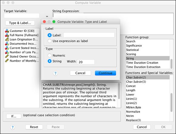
FIGURE 10-9: The Type and Label dialog.
If you're comfortable with these more complex expressions, it's a good indication that you'll be comfortable with Syntax as well, although moving from complex functions in the expression box to writing programs in the Syntax window still requires a small leap in SPSS knowledge. We cover programming with Syntax in Chapters 26 and 27. If writing code is not your preferred way to work with SPSS, you can generally avoid it and stick to the menus. We discuss the tradeoffs in Chapter 26.
Calculating Lags
A common task is to lag, or shift, values using the LAG function. Perhaps the most common example is transactional data or time series data. The brief example in this section uses the stock_lag dataset, which is available on the book's website (www.dummies.com/go/spss4e) and shows two simple expressions.
Table 10-5 shows the stock closing price for each date. You can also see that the lag of the closing price places the previous day’s value in a new column. This allows you to calculate Close-Lag(Close), which represents the price change. For instance, on Tuesday, August 4, our fictional stock rose to $83.45, representing an increase of $1.67 over the previous day's closing price.
TABLE 10-5 LAG() Function Results
|
Stock_Ticker |
Date |
Close |
LAG(Close) |
Close-LAG(Close) |
|
X123 |
08/03/2020 |
$81.78 |
. |
. |
|
X123 |
08/04/2020 |
$83.45 |
81.78 |
1.67 |
|
X123 |
08/05/2020 |
$83.95 |
83.45 |
.50 |
|
X123 |
08/06/2020 |
$82.25 |
83.95 |
-1.70 |
|
X123 |
08/07/2020 |
$82.50 |
82.25 |
.25 |
You can perform a lag also by using the Transform ⇒ Shift Values menu.