
4
Cost of Delay
Donald Reinertsen, in his book, The Principles of Product Development Flow, introduced the concept of “Cost of Delay (CoD)” in software development. It's a simple yet elegant concept. CoD is the loss in income if a project is delayed one month. He also showed that prioritizing projects by CoD divided by cycle time, which he refers to as “Weighted Shortest Job First” (WSJF), results in the lowest “Net CoD,” which is the cumulative cost of delay for a set of projects that must be prioritized because of development resource constraints.
For product managers, Net CoD is the same as opportunity cost. Opportunity cost is the profit or income lost by choosing one alternative over the other. Given two development projects P1 and P2, prioritization of P1 defers income from P2, which would be referred to as the opportunity cost for doing P1 first. The role of product management in Agile is to define and prioritize R&D work for the backlog to minimize opportunity cost. This chapter illustrates how Reinertsen's CoD and WSJF principles can accomplish that.
Although CoD, or opportunity cost, has always existed in software development, it has been difficult to quantify. Features with unjustified financial value have traditionally been bundled into large periodic releases. However, the importance of adopting a CoD approach has substantially increased today because of the ability to develop and release value faster with Agile development. Increasing the number of releases within a planning period increases the permutations of project development order. For example, breaking an annual release into four increments results in 24 unique development order permutations. Which one maximizes R&D Return on Investment (ROI)? That will be the case where the Net CoD is lowest.
Software organizations have found it difficult to implement WSJF prioritization because Reinertsen's formula is based on projects with constant CoD. Total income generated by a software release usually follows an adoption ramp defined by the classic “S‐curve” (Figure 4.1). Initial market penetration is low, followed by rapid adoption and then saturation. This is true for new products and software upgrades. It is even true for subscription pricing models where the curve is determined by deployment rates.
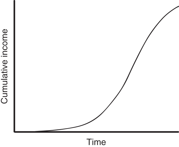
Figure 4.1 S‐curve income profile.
This chapter introduces three methods for estimating Net CoD for nonlinear income profiles, each with increasing complexity and varying accuracy. The third method is the most accurate, but it requires significant computing power to calculate the permutations of backlog Investment order. It is included for completeness, but any of the first two methods should be adequate. I stress not getting hung up about WSJF accuracy. The lack of precision in development effort and financial estimates used in the calculation exceeds the variations based on the model chosen. The main goal of WSJF is to provide a clear financial trade‐off between development effort and income forecasts. This is a discussion that normally doesn't take place in software development.
The last section compares WSJF prioritization with traditional ROI prioritization.
4.1 Weighted Shortest Job First (WSJF)
WSJF was historically used in computing to prioritize batch jobs. Batch job priorities were weighted in terms of importance and estimated execution time. WSJF was calculated by dividing the weighted importance by estimated execution time.
WSJF for software projects can be calculated using Reinertsen's formula:
where cycle time is the duration of the project. Projects that have a higher CoD generate higher income per unit time, which means that delays are more expensive. We want to prioritize projects with the highest CoD and the shortest development time, generating the maximum income from constrained R&D resources.
4.1.1 Cost of Delay Basics
Let's start with Reinertsen's description of CoD from The Principles of Product Development Flow [1]. The chart assumes three software projects with different CoDs and cycle times. The example assumes that each project generates uniform income per month. Income is used throughout this book in relation to CoD instead of profit. Either could be used, but profit calculations add another layer of complexity beyond what is necessary for software project prioritization.
Reinertsen uses the example of three projects with different CoD and cycle times (Table 4.1).
Reinertsen depicts the projects in Figure 4.2 to show accumulated Net CoD for project order A, B, and C.
Table 4.1 Reinertsen project CoD example.
| Project | Cycle time | CoD | CoD/cycle time |
|---|---|---|---|
| A | 1 | 10 | 10 |
| B | 3 | 3 | 1 |
| C | 10 | 1 | 0.1 |
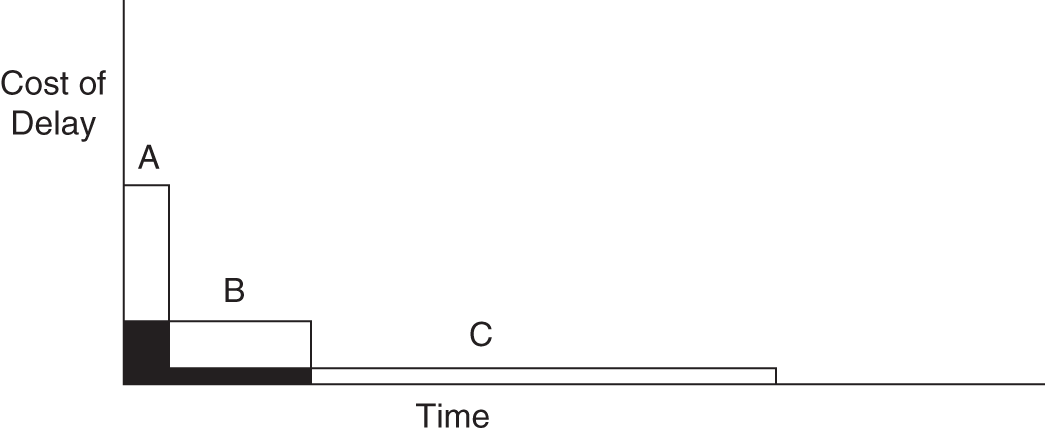
Figure 4.2 Reinertsen project Cost of Delay (CoD) example order A, B, C. Used with permission of Donald Reinertsen.
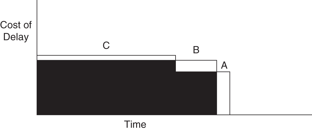
Figure 4.3 Reinertsen project CoD example order C, B, A. Used with permission of Donald Reinertsen.
Table 4.2 Project WSJF productivity example.
| Project | Time (mo) | CoD ($K/mo) | WSJF |
|---|---|---|---|
| P1 | 3 | 30 | 10 |
| P2 | 9 | 45 | 5 |
Project A generates cumulative income over a period determined by its CoD multiplied by time. In the first example, Project A is developed first, delaying the start of development of Projects B and C by the development duration of Project A. The Net CoD for developing Project A first is the sum of the Costs of Delay of Projects B and C multiplied by the development duration of Project A, represented by the first dark rectangle on the left of the chart. Project C is delayed while Project B is developed, creating the Net CoD depicted by the second dark rectangle. There are no projects delayed while Project C is being developed.
Figure 4.3 shows the reverse project order. It is the worst case because higher income per month is deferred for longer periods of time.
Reinertsen asserts that Net CoD is minimized by prioritization by WSJF for the case of linear income ramps (constant CoD). Net CoD is incurred in software development any time there is a defined set of projects that cannot start at the same time. Of course, this is the typical case. There is always more work than can be developed in parallel by constrained R&D resources. CoD can also be viewed from the perspective of income generation. Consider an example of two projects of different durations and Costs of Delay as shown in Table 4.2.
4.1.2 Example
The WSJF calculation shows that P1 should take priority. Figure 4.4 shows the cumulative net income when we develop in the reverse WSJF order with P2 first.
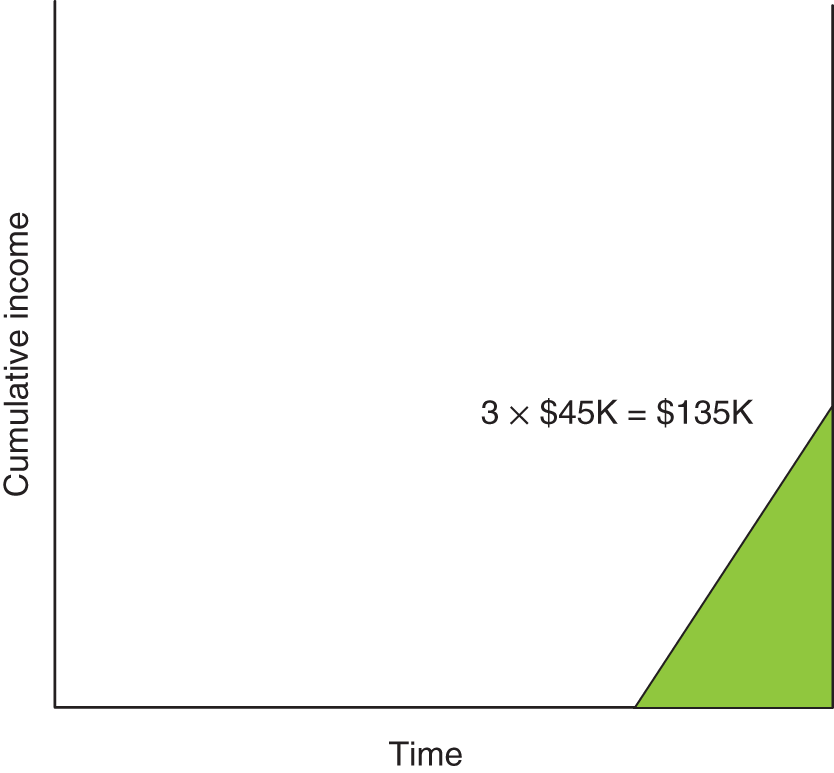
Figure 4.4 Reverse Weighted Shortest Job First (WSJF) prioritization income generation.
P1 income of $45K per month starts after completion of P2 and generates $135K over the last three months of the year. P2 adds $30K per month starting at the end of the year for a running total of $75K per month beyond one year.
The cumulative income profile for WSJF prioritization is shown below (Figure 4.5). In this case, the income of $30K per month from P1 starts after three months and contributes $270K for the year. The income beyond one year is the same as in the first example.
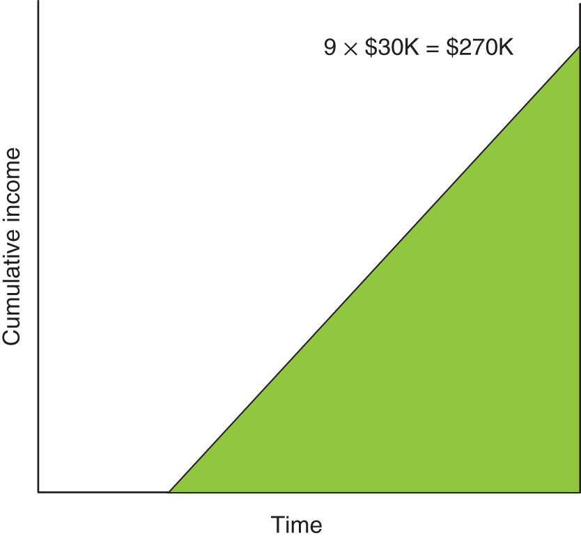
Figure 4.5 WSJF prioritization income generation.
Total productivity is Value Out/Value In. It's simply the income or profit generated by a software release divided by the cost to develop the software. Productivity can be calculated for both cases. R is total productivity, I is the income for the year, and C is the development cost for both projects.
Development cost cancels out when we take the ratio of productivity.

For this example, total productivity improves by a factor of 270/135 = 200%.
This is a simplistic view that ignores software capitalization, taxes, and NPV. It also assumes that income is the same as profit. The engineering organization would need to double its productivity to attain the same result with the reverse WSJF prioritization.
4.1.3 WSJF Proof
We can prove that WSJF prioritization optimizes income for the case of linear income ramps assumed in Reinertsen's formula. Consider two projects P1 and P2, each with CoD and duration T. Figure 4.6 shows the cumulative income for the case where P2 is done first. The total period is the sum of the durations for both projects.
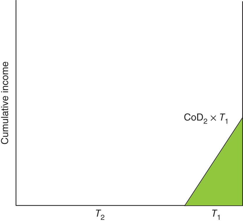
Figure 4.6 Cumulative income with P2 first.

Figure 4.7 Cumulative income with P1 first.
Figure 4.7 shows the case where P1 is completed first.
P1 should be prioritized when greater income is generated within the same period. The income generated with P2 developed first is the CoD of P2 multiplied by the cycle time of P1. Income generated when P1 is developed first is the CoD of P1 multiplied by the cycle time of P2. P1 should be prioritized when
By cross multiplying we get Reinertsen's WSFJ formula.
It's interesting to look at the units of the WSJF calculation. The units are in currency per unit time squared. We can consider currency per unit time to be analogous to velocity of an object. Velocity is in terms of distance per unit time. Acceleration units are distance per unit time squared. For example, acceleration due to gravity is 9.8 m/s2, which means that your falling speed, neglecting friction, increases by 9.8 m/s every second. WSFJ represents income acceleration. A WSJF of $100K/month2 means that income is deferred by $100K per month for every month of delay. Projects with higher WSJF accelerate income.
Before moving on to WSJF calculation methods, I want to stress something.
The most valuable aspect of WSJF in Agile development is that it establishes incentives for the Minimum Marketable Feature Set (MMFS)
It's not so much about having a precise calculation of CoD and WSJF. Dividing income generation by cycle time prioritizes projects that can generate the greatest value that can be developed in the shortest cycle time, which encourages the least functionality required to meet financial targets.
4.1.4 CoD and Net Present Value (NPV) Prioritization Methods
I often hear product managers say that CoD is just an NPV problem. They recognize that the income in our example above is only different for the first year, and then $900K per year is generated after that at a rate of $75K per month. The cumulative income is shown in Table 4.3.
Why then prioritize by WSJF? It just looks like an issue of income timing which can be addressed by NPV calculations. Before answering the question, I'll explain NPV for those of you not familiar with the term.
NPV accounts for what is called the “time value of money.” NPV is used to compare alternatives that return money at different times in the future. A dollar invested today does not have the same value as a dollar earned three years from now.
For example, assume a dollar is invested at an annual return of 10% paid out at the end of each year. It would be worth $1.00 × (1 + 0.10) = $1.10 after the first year. After the second year, it would be worth $1.10 × (1 + 0.10), which is $1.00 × (1 + 0.10)2. After three years the value is $1.00 × (1 + 0.10) × (1 + 0.10) × (1 + 0.10) = $1.33 which is $1.00 × (1 + 0.10)3. So, if you could get a return of 10% on your money, $1.00 you expect to receive in three years is only worth $1.00/(1 + 0.1)3 today, which is an NPV of $0.75.
The general NPV formula is
where R is the net cash flow at time t and i is the “discount rate” for the period t.
The discount rate is the same as an interest rate in the example above. However, companies calculate the discount rate based on how they value money. Their ability to raise cash is limited by financial considerations like current debt and investor risk. Your CFO determines the discount rate for your organization. The discount rate is unique to your company and is typically higher than prevailing interest rates. Otherwise, investors may as well secure their money in banks.
Table 4.3 CoD cumulative non-discounted income example ($K).
| Year 1 | Year 2 | Year 3 | Year 4 | Year 5 | |
|---|---|---|---|---|---|
| P2 First | $135 | $1035 | $1935 | $2835 | $3735 |
| P1 First | $270 | $1170 | $2070 | $2970 | $3870 |
| Increase | 100% | 13% | 7% | 5% | 4% |
The NPV formula is used to calculate your mortgage rate payments. It determines the monthly payments required to reduce the NPV of your mortgage to zero by the end of the mortgage, based on the mortgage interest rates. Companies don't have access to the low interest rates of safe mortgages backed by property. They get their funding from a wide variety of capital sources like business loans, corporate bonds, and stock sales. Their NPV discount rate is based on the Weighted Average Cost of Capital (WACC) which can be different for each company.
A 2019 KPMG study [2] states that the average WACC for all industries was 6.9%. Companies calculate WACC based on their access to capital and use it as the discount value in NPV calculations. The technology sector average WACC was 8.1%, which is applied to Table 4.4 to calculate NPV for our example cashflow.
The percentages increase slightly in each year. However, it still seems like it's not worth the effort to calculate WSJF and we can just use NPV to prioritize projects as we've always done. It turns out that the importance of WSJF prioritization increases substantially for Agile development.
NPV calculations assume you can forecast income over a long period of time. We know this is a dangerous assumption in today's dynamic world of software development. Agile development enables competitors to rapidly take advantage of new opportunities. Platform as a Service (PaaS) offerings like Microsoft Azure and Amazon Web Services enable startups to quickly build enterprise applications with virtually unlimited scalability that can replace enterprise software. Companies want to minimize exposure with software releases with short payback periods, usually less than three years.
NPV prioritization does not significantly differentiate between projects with different cycle times over a multiyear planning period. However, consider using WSJF prioritization for new projects every year. In this case, the income from new projects in each year is doubled.
In summary, traditional NPV calculations do not sufficiently factor in the cycle times of Agile projects approaching weeks or months. WSJF prioritization should be used. However, we will consider NPV in one or our WSJF calculation methods discussed in Section 4.3.2.
Table 4.4 CoD discounted cumulative income example ($K).
| Year 1 | Year 2 | Year 3 | Year 4 | Year 5 | |
|---|---|---|---|---|---|
| P2 First | $135 | $895 | $1608 | $2267 | $2876 |
| P1 First | $270 | $1020 | $1732 | $2391 | $3001 |
| Increase | 100% | 14% | 8% | 6% | 4% |
4.2 Nonlinear Income Profiles
The WSJF formula doesn't work in the case where the rate of income generation is a nonlinear function of time, which is true in most cases for software releases. It's not possible to cross multiply Reinertsen's formula to calculate a value for WSJF independent of the cycle times of other projects. We need a practical way to calculate WSJF for non-linear income profiles, like the S-curve in Figure 4.1.
4.3 CoD for Nonlinear Cumulative Income Profiles
Scaled Agile Framework (SAFe) claims to use WSJF, but they have reverted to a subjective weighting system based on “user‐business value,” “time criticality,” and “risk reduction‐opportunity enablement value.” There is no mathematical correlation with Reinertsen's WSJF calculation. And the weights are subjective, open to opinion, and political influence.
There are three methods described in this section to prioritize Investments with nonlinear income profiles:
- Payback Period CoD Method
- Third‐year Income Slope CoD Method
- CoD Computation Method
4.3.1 Payback Period CoD Method
There is a relationship between CoD and payback period. A project with a CoD of x dollars per month reaches its payback point when CoD multiplied by time equals the development Investment. Therefore, CoD for software development can be approximated by the project labor cost divided by the payback period. For example, a project that costs $360K with a three‐year payback would need to return an average of $360K/36 months = $10K per month. CoD can be estimated as $10K per month. This simple calculation provides a linear approximation for non-linear income profiles.
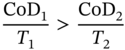
4.3.2 Third‐Year Income Slope CoD Method
This is the simplest and recommended approach. It assumes a three‐year planning period to support prioritization of projects that can start within the next year. CoD is the rate at which income is shifted beyond three years.
Cycle time and income projections beyond three years are questionable. And with Agile development, it's likely that any projects planned within three years will change. In fact, the value of WSJF prioritization is not planning the optimal development order for a set of Agile projects over the next five years. It is to determine which project to start next. We want to look at the rate at which income will be shifted out of the three-year planning period depending upon which projects we start next. It is a dynamic calculation based on today's view.
Consider the S‐curve case shown in Figure 4.8.
The rate at which income is deferred beyond three years can be approximated by the average slope of the curve between Years 2 and 3. This linear approximation applies for delays of up to one year. Figure 4.9 shows that a six‐month delay places the linear approximation at the edge of the three‐year boundary.
The linear approximation results in a simple way to calculate monthly CoD. It is simply the income generated in the third year divided by 12.
Another reason for using a three‐year planning period is that NPV impacts are relatively small compared with the estimation error of income projections and can be ignored. Figure 4.10 shows the effect of excluding NPV from multi‐year income projections.
The lines represent discount values ranging from 6% to 10% per year. For example, the NPV of $1000 received in Year 2 at a rate of 10% is $1000/(1 + 0.10) = $909. Neglecting the cost of money creates an error of (1000 – 909)/1000 = 9%. At an average discount of 8% typical of the high‐technology sector within the three‐year period, the error is less than 15%, well within the accuracy of income projections three years out.
The third‐year cumulative income slope method provides sufficient accuracy for project delays of up to one year. The CoD approximation is effective for determining the next software increment to be released in Agile development.
If you need to consider income beyond three years, you can use the NPV of the income beyond three years for all projects. In this case, the CoD is the NPV divided by 12 months. However, a risk factor should be incorporated before calculating NPV that far out.
Figure 4.8 Third‐year income CoD calculation.
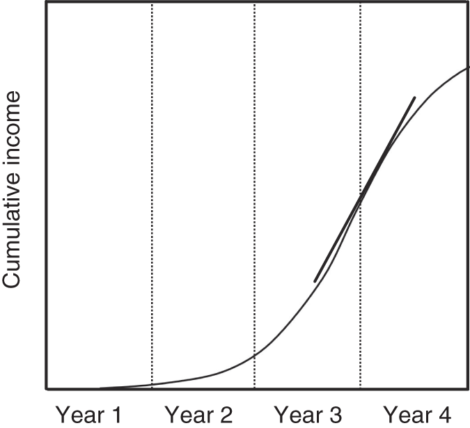
Figure 4.9 Third‐year income slope with delay of 2.5 years.
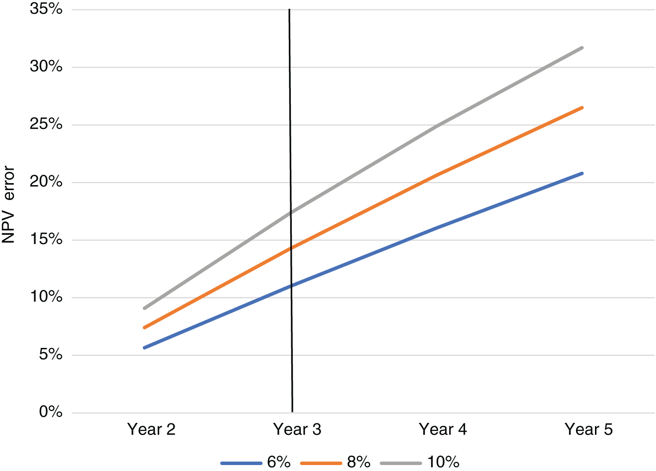
Figure 4.10 Net Present Value (NPV) error based on discount period.
Consider the following project annual income profile (Table 4.5):
Assume a discount rate of 8%. Years 4 and 5 are discounted for the number of years beyond Year 3 after applying the risk factors.
Table 4.5 Net Present Value (NPV) beyond three years example.
| Year 1 | Year 2 | Year 3 | Year 4 | Year 5 | |
|---|---|---|---|---|---|
| Income ($K) | 20 | 60 | 90 | 120 | 200 |
| Risk Discount | 20% | 50% | |||
| Risk‐Adjusted Income ($K) | 20 | 60 | 90 | 96 | 100 |
NPV should be calculated for the five‐year period for all projects to be prioritized.
The third‐year slope method can result in a CoD of zero, as shown in Figure 4.11.
For example, a modular deployment may be deployed within a period of two years. What is the priority with a CoD and WSJF of zero?
This answer is nonintuitive. If your goal is to optimize income within a three‐year planning period, projects that don't generate income in the third year can be prioritized lower, because the income will still be captured within the planning period.
4.3.3 CoD Computation Method
Net CoD can be calculated for any set of projects where the income profile can be modeled as a function of time. Consider two projects P1, P2 with the nonlinear income ramps developed in project order P1, P2 with cycle times T1 and T2. The Net CoD for delaying P2 by the cycle time T1 is the income that would have been generated by P2 up until the time when P1 is complete. Figure 4.12 shows the cumulative income for each project, with P2 delayed by three quarters by the development of P1. Each income profile is modeled with a function of the form:

Figure 4.11 S‐curve for income returned within two years.
Now consider three projects. The Net CoD for order P1, P2, and P3 is:
The income generated by f3 starts after both P1 and P2 are complete.
If the order is reversed, the Net CoD is:
The Net CoD for a set of n projects must be calculated n! times because there are n! permutations of project order for n projects. Appendix A provides an example of three projects where the income curves are in the form:
Any function of time will work, including the logistics curve function (S‐curve) described by
| L | = | maximum value |
| k | = | slope of the curve at the inflection point, also called the logistics growth rate |
| T0 | = | the time value at the inflection point |
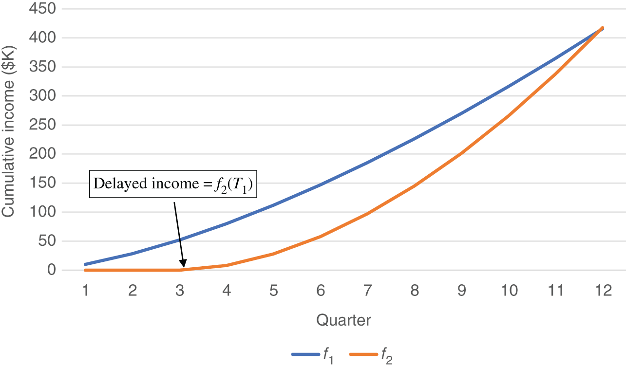
Figure 4.12 Cumulative income based on project order.
We can prove Reinertsen's linear WSJF formula for the case of linear income ramps when income is a constant multiplied by time:
where C is the CoD. P1 should be prioritized when the income delayed for order P1, P2 is less than the delayed income of order P2, P1:
which is the same as the WSJF formula:

4.4 WSJF and Traditional Finance
WSJF can be related to traditional finance terms used in project planning. This section looks at ROI, IRR, and payback period.
4.4.1 ROI
ROI is income returned over a planning period minus the investment divided by the investment.
Table 4.6 shows the annual income generated over a five‐year planning period for the two different development orders of the projects P1 and P2 in Table 4.2. Both projects complete in the first year so R&D investment for Year 1 is the same in both cases. Income in Years 2 and 3 is based on $75K per month after the first year for both cases.
Table 4.6 Three‐year income projections for WSJF example.
| Project order | Year 1 | Year 2 | Year 3 |
|---|---|---|---|
| P1 First | $270K | $900K | $900K |
| P2 First | $135K | $900K | $900K |
Many companies impose a minimum payback period by which they must recover project investment. Income in later years is more difficult to predict, especially in the dynamic world of software development. Therefore, companies want to reduce risk by recovering their R&D costs within a shorter period. The exact value is established by your CFO. A payback of one year will be assumed in this example. Development cost is equal to the sum of the first‐year income which is $405K.
Table 4.7 shows ROI after each year:
Table 4.7 Return on Investment (ROI) impact of WSJF prioritization.
| Project order | After Year 1 | After Year 2 | After Year 3 |
|---|---|---|---|
| P1 First | −33% | 189% | 411% |
| P2 First | −67% | 156% | 378% |
The table demonstrates that WSJF prioritization provides return on an investment sooner but approaches the same value with increasing planning periods. However, it significantly decreases ROI risk because returns are more predictable in earlier years.
4.4.2 Investment Rate of Return (IRR)
IRR is another financial calculation impacted by WSJF prioritization. IRR is a common method for comparing the financial value of projects. IRR is defined as a “discount rate” that makes NPV zero in a discounted cash flow analysis. The interest on your mortgage is the IRR. For example, the IRR of a 30‐year mortgage is the interest rate to pay off the mortgage after 30 years of monthly payments. If you were a mortgage lender, you would want to receive the highest IRR possible.
Excel calculates IRR based on a series of cashflows. Table 4.8 shows the IRR for both orders of P1 and P2.
Table 4.8 IRR impact of WSJF prioritization.
| Project order | After Year 2 | After Year 3 |
|---|---|---|
| P1 First | 567% | 655% |
| P2 First | 233% | 314% |
We see a similar pattern where near‐term IRR is improved but converges over time.
4.4.3 WSJF Versus ROI Prioritization
Companies using traditional ROI project prioritization are losing millions of dollars in opportunity cost with Agile development. Consider five Investments with development costs and Costs of Delay as shown in Table 4.9. As in traditional planning, ROI is calculated separately for each Investment to determine priorities. Over the 12‐quarter planning period, Investments generate income at the rate determined by CoD. For example, Investment 1 returns income of $25K per quarter × 12 quarters = $300K with a development cost of $100K so ROI is ($300 − $100K)/$100K = 200%.
Table 4.9 ROI prioritization example.
| Investment | Development cost ($K) | Income ($K/quarter) | ROI (%) |
|---|---|---|---|
| Investment 1 | 100 | 25 | 200 |
| Investment 2 | 75 | 35 | 460 |
| Investment 3 | 50 | 30 | 620 |
| Investment 4 | 130 | 40 | 269 |
| Investment 5 | 90 | 45 | 500 |
Table 4.10 WSJF prioritization example.
| Investment | Cycle time (quarters) | CoD ($K/quarter) | WSJF |
|---|---|---|---|
| Investment 1 | 1 | 25 | 25 |
| Investment 2 | 2 | 35 | 18 |
| Investment 3 | 2 | 30 | 15 |
| Investment 4 | 3 | 40 | 13 |
| Investment 5 | 4 | 45 | 11 |
Investment ROI priority order is 3, 5, 2, 4, 1.
We now consider cycle time and apply the quarterly income as CoD to calculate WSJF (Table 4.10).
WSJF prioritization shows the optimal Investment order is 1, 2, 3, 4, 5.
Figure 4.13 plots cumulative income by quarter for the ROI and WSJF priority order cases and adds a line for the worst-case reverse WSJF order:
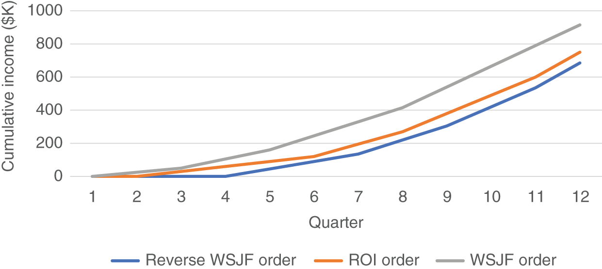
Figure 4.13 Cumulative income by prioritization method.
As expected, WSJF prioritization produces the greatest income of $950K within the planning period. ROI prioritization generates $750K. The worst case of reverse WSJF order results in $685K.
Three‐year ROI can be calculated for each case (Table 4.11).
Table 4.11 ROI comparison based on prioritization method.
| Prioritization method | Three‐Year ROI |
|---|---|
| WSJF | 106% |
| ROI | 69% |
| Reverse WSJF | 54% |
This is only one example. But it demonstrates that ROI prioritization is likely to result in an ROI somewhere between what could be attained with WSJFprioritization and the worst case of reverse WSJF prioritization. ROI prioritization is not likely to result in the optimal ROI, especially with the larger number of permutations of Agile projects.
4.5 Summary
- CoD is the profit or income lost by delaying a software project by a unit of time.
- Software projects prioritized by WSJF optimize income over a planning period by minimizing Net CoD.
- WSJF prioritization has become more important with shorter release cycles enabled by Agile development.
- Reinertsen's WSJF prioritization formula is based on linear income ramps. Software release income ramps are more likely to be nonlinear.
- The greatest benefit of WSJF is establishing a prioritization target to encourage smaller development increments of higher value.
- Multiple methods are available for calculation of CoD for nonlinear income profiles.
- WSJF prioritization can significantly improve development productivity and ROI using currently available resources and development practices.
- Relationships between CoD and traditional software planning metrics like ROI and IRR demonstrate how WSJF prioritization provides earlier returns.
References
- 1 Reinertsen, D.G. (2009). The Principles of Product Development Flow. Celeritas Publishing.
- 2 KPMG, Cost of Capital Study, 2019. https://home.kpmg/de/en/home/insights/2020/10/cost-of-capital-study-2020.html.