4

Boundary Layers

In Section 3.6, we saw that the basic effect of viscosity is to exert shear stress, and that when that is combined with a no-slip condition at a solid surface, it leads to vorticity that originates at the surface, is convected downstream, and diffuses outward. (In Section 4.2.4, we'll look at this in detail and see that some parts of a surface act as sources of vorticity, and others act as sinks, but that the net result is that there is always some vorticity convected along next to a solid wall.) In Section 3.8.2, we saw that irrotational flow tends to remain irrotational until viscosity has had a chance to work on it. The upshot is that flows around bodies at high Reynolds numbers acquire a natural global structure: an inner vortical region where viscosity is important, consisting of the boundary layer next to the surface and the wake downstream, surrounded by an outer flow that is effectively irrotational and that behaves as if it were inviscid. This basic pattern was not generally understood until Prandtl (1904) explained it and proposed his approximate theory for the flow in the boundary layer.

In this chapter, we'll take a detailed look at the physics of the flow in the boundary layer, in preparation for a more global discussion of the whole flowfield in Chapter 5. This ordering of the discussion is convenient because it turns out that the boundary layer and the outer flow interact only through a relatively simple set of boundary conditions at their interface, and everything of interest in the physics of the boundary layer can be discussed in general terms without our having to know much about the outer flow. On the other hand, our later discussion of the global flow will refer often to what goes on in the boundary layer. Boundary-layer specialists like to joke (only half joke, actually) that the boundary layer is the most important part of the flow because it's the only part that touches the body.

When the Reynolds number is sufficiently high, the boundary layer remains relatively thin, unless it separates from the body “prematurely,” that is, ahead of the tail of a body or the trailing edge of a wing. Within the thin attached boundary layer, Prandtl's simplified versions of the Navier-Stokes (NS) equations often apply, along with special boundary conditions through which the boundary layer and the outer inviscid flow interact. These equations and the many methods for solving them constitute the subdiscipline of fluid mechanics called boundary-layer theory. The terminology can be confusing, for example, when it is sometimes implied that the viscous flow near the surface ceases to be a “boundary-layer flow” when it fails to satisfy the assumptions of boundary-layer theory. We won't take that narrow view here. Most of the physical boundary-layer phenomena we'll discuss in this chapter don't depend on the validity of boundary-layer theory. However, the theory does provide helpful insights into why boundary layers behave as they do, and it is sufficiently accurate, enough of the time, that it is useful for quantitative analysis as well. And, of course, the theory played a huge role in the history of our understanding of viscous effects at high Reynolds numbers.

In this chapter, we'll limit our attention to steady boundary-layer flows. We'll get to the specifics of the theory in Section 4.2, after discussing the general physical aspects of 2D and 3D boundary-layer flows in Section 4.1. In much of the literature, 2D boundary layers and 3D boundary layers are treated as separate universes. To emphasize the common ground these two universes share, we'll take a different tack here, and in the discussion in Sections 4.1 and 4.2, we'll keep 2D and 3D integrated. Topic by topic, we'll introduce ideas in 2D and then discuss what has to be added to go to 3D. Then, in the remaining sections, we'll deal with transition and turbulence, control of flow separation, heat transfer, compressibility, and surface roughness.

4.1 Physical Aspects of Boundary-Layer Flows

The boundary layer is a thin sheet of flow close to the surface, so it's natural to imagine following its progress along the surface and using time-like terminology to describe its development even when the flow is actually steady. And we'll use this kind of time-like terminology to refer to the boundary layer as a whole, even though fluid parcels flowing along at different distances from the surface move at different speeds and thus experience different transit times. This is an example of the “pseudo-Lagrangian viewpoint” we discussed in Section 3.4.7. Imagining a steady flow in this way is especially appropriate in the case of a boundary layer, because, as we'll see in Section 4.2, a boundary layer flow has the character of an initial-value problem. You'll note that many discussions of boundary-layer flows, including those in this chapter, use time-like terminology freely.

4.1.1 The Basic Sequence: Attachment, Transition, Separation

Let's look first at the major milestones that mark the development of a 2D boundary layer as it flows along the surface of a body. The development starts where the flow first attaches at or near the front of the body and ends where the boundary layer finally leaves the body and becomes part of the viscous wake. In between, the boundary layer will usually undergo transition from laminar to turbulent, except in special cases at low Reynolds number, and it may also undergo intermediate separation and reattachment.

The least complicated type of 2D attachment occurs at a stagnation point, at or near a blunt leading edge, as shown in Figure 4.1.1a. The velocity u_e just outside the boundary layer initially increases linearly in both directions from such a stagnation point, and the boundary layer in the neighborhood is always laminar. In the region of linear acceleration, the boundary-layer development is described by one of the special similarity solutions to the equations, as described in Section 4.3.2. The thickness of the boundary layer remains constant until u_e deviates from its initial linear distribution.

If the leading edge is sharp, the situation is not always simple. For supersonic flow or for one particular angle of attack in subsonic flow, the flow can attach directly to the sharp leading edge, as shown in Figure 4.1.1b. At other angles of attack in subsonic flow, the attachment will be either above or below the leading edge, as in Figure 4.1.1c, with local behavior around the attachment point like that of Figure 4.1.1a, and there will be a separation at the leading edge with at least a short bubble of recirculating flow downstream.

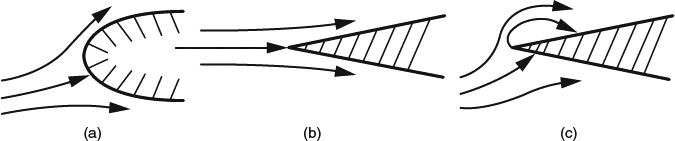
Figure 4.1.1 Types of initial boundary-layer attachment in 2D. (a) At or near a blunt LE (b) Directly on a sharp LE. (c) Near a sharp LE

The final separation of the boundary layer from a 2D body can take place either from a sharp trailing edge, as in Figure 4.1.2a, or from a smooth part of the surface, as in Figure 4.1.2b. Separation from a smooth surface raises interesting physical issues that we'll discuss further in Section 4.1.4. Between the initial attachment and the final separation, a boundary layer usually undergoes transition from laminar to turbulent, a process we'll discuss in some detail in Section 4.4.1.

Separation with subsequent reattachment can take place from a sharp leading edge, as in Figure 4.1.1c; from a smooth surface, as in Figure 4.1.3a,b; or from a sharp corner at the edge of a “cove,” as in Figure 4.1.3c. In a smooth-wall separation bubble like that in Figure 4.1.3a, the reattachment is usually precipitated by transition to turbulent flow, with its associated rapid increase in shear stress. For reattachment to happen without transition, the separation bubble would generally need to occupy a dip in surface, as in Figure 4.1.3b, because reattachment of a laminar boundary layer requires a favorable pressure gradient, as would occur as the flow exits the dip. Pressure gradients also play an important role in smooth-wall separation, as we'll see below.

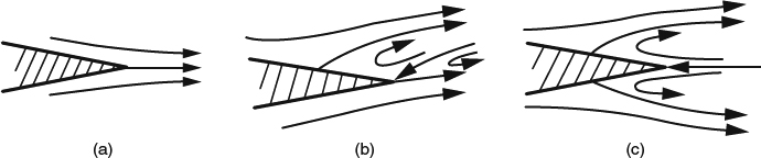
Figure 4.1.2 Types of final 2D boundary-layer separation in 2D. (a) Separation from sharp TE. (b) Single separation from smooth surface and into the wake. (c) Double separation from smooth surface and into the wake

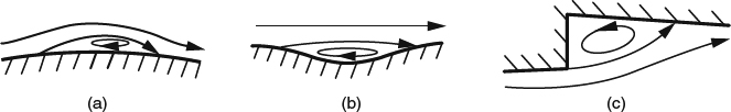
Figure 4.1.3 Types of boundary-layer separation with subsequent reattachment in 2D. (a) Laminar separation from a smooth surface with reattachment triggered by transition to turbulent flow. (b) Laminar separation and laminar reattachment in a dip in the surface. (c) Separation at the sharp edge of a “cove”

Note that the word separation connotes two different aspects of a flow's topological structure. First, separation in general involves some flow leaving the surface and forming a shear layer that is at least somewhat “separated” from the surface. Second, a line of separation on the surface divides the surface into “separate” regions, from which the flow along the surface converges from different directions (By “flow” we are referring either to flow a short distance off the surface or, loosely, to the surface shear stress). This is an idea we'll return to in our discussion of 3D separation in Section 4.1.4.

3D boundary-layer flows run the gamut from nearly 2D at one extreme to very different from 2D at the other. In some situations, we can view a 3D flow in cross sections and see the same patterns of attachment and separation that we saw in 2D flows in Figures 4.1.1–4.1.3. But the additional dimension in 3D makes many other patterns of attachment and separation possible as well.

Note that in 2D flows the attachment and separation points are actually lines that extend to plus and minus infinity in the “spanwise” direction. In 3D flows, we can have singular points of attachment and separation, and these are often accompanied by what we commonly call attachment lines and separation lines that can form complicated patterns on the surface of the body. These terms are very useful for discussions of flow patterns, but we should note that they aren't mathematically precise. In real flows around finite bodies, the flow structures that we commonly call attachment lines and separation lines are not uniquely defined lines or curves in the mathematical sense. They are actually bands of finite width, loosely defined by either strong flow convergence toward the body (attachment) or strong diverge away from it (separation), but for practical purposes, they are often sufficiently narrow that it isn't grossly inaccurate to refer to them as “lines.”

This issue will become clearer when we discuss what the boundary-layer velocity field looks like in more detail locally in the neighborhood of separation in Section 4.1.4. Then we'll discuss the global topology of points and “lines” of attachment and separation on the body surface in some detail in Section 5.2.3.

4.1.2 General Development of the Boundary-Layer Flowfield

Now let's look at the general features of the boundary-layer velocity field, time-averaged if the flow is turbulent. The velocity in the boundary layer is nearly parallel to the surface. It varies relatively slowly along the surface, but much more rapidly in the direction normal to the surface, in a distribution called the velocity profile.

Typical velocity profiles for 2D laminar and turbulent flow are shown in Figure 4.1.4. In both cases, the velocity starts at zero at the surface, in keeping with the no-slip condition, and gradually approaches a distribution consistent with an inviscid outer flow. In the first-order theory that we'll discuss in Section 4.2.1, and therefore in this discussion, we'll ignore the slope of the inviscid velocity distribution in the outer flow and assume that the slope of the boundary-layer profile goes to zero. The boundary between the viscous boundary layer and the effectively inviscid outer flow is often referred to as the boundary-layer “edge,” though in fact it is indistinct. Any definition of the boundary-layer edge is thus arbitrary. The usual choice is the point at which the velocity reaches 99% of its outer-flow value, and the term boundary-layer thickness usually refers to the distance from the surface to this 99% point. Because the slope of the velocity profile is small there, the determination of boundary-layer thickness in this way is sensitive to small errors in the determination of the velocity profile, especially in the turbulent case, and the difficulty is compounded if the distribution of velocity in the outer flow has significant slope.

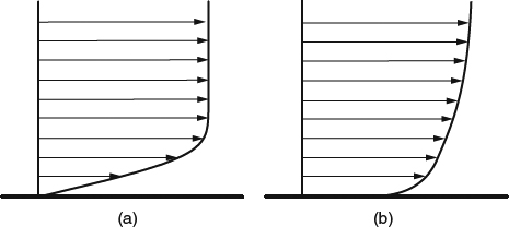
Figure 4.1.4 Typical 2D boundary-layer velocity profiles. (a) Laminar. (b) Turbulent

In a laminar constant-property boundary layer the viscosity μ is constant, so that the shear stress in 2D is just proportional to ∂u/∂y. Given the shape of a laminar velocity profile in Figure 4.1.4a, we can see that the shear stress starts at zero at the outer edge of the boundary layer and increases as the wall is approached. The value of μ∂u/∂y at the wall itself is the shear stress τ_w transmitted from the flow to the surface and is referred to as the skin friction. This terminology is a bit misleading, because it evokes an image of relative motion between the fluid and the surface, as in mechanical friction. But remember that with the no-slip condition at the surface, there is no relative motion, and that this is “friction” only in the sense that a shear force is exerted on the surface.

In a compressible boundary layer or a turbulent boundary layer the relationship between τ and ∂u/∂y is more complicated, but τ_w is still proportional to ∂u/∂y at the wall. Though a turbulent boundary layer is typically much thicker than a laminar one, the turbulent layer has a much larger gradient ∂u/∂y at the wall and thus much higher skin friction. We'll consider turbulent boundary-layer flow in detail in Section 4.4.2 and compressible flow in Section 4.6.

A streamwise pressure gradient ∂p/∂x causes additional acceleration that affects the shape of the velocity profile. Because ∂p/∂x tends to be nearly the same across the thickness of a boundary layer, it contributes nearly the same incremental material (Lagrangian) acceleration to fluid parcels regardless of distance from the wall. In Equation 3.2.2, we saw that a given Lagrangian acceleration requires larger ∂u/∂x when u is small than when u is large. Thus the bottom of the boundary layer, where u is small, responds to ∂p/∂x with a more rapid spatial rate of change of u (larger ∂u/∂x) than does the outer part of the boundary layer. As a result, a positive pressure gradient reduces the velocity at the bottom of the profile more than at the top, as shown in Figure 4.1.5a, and pushes the flow closer to separation, which we'll discuss in Section 4.1.4. Because of this association with the approach to separation, a positive pressure gradient is often called an adverse pressure gradient. A negative, or favorable pressure gradient has the opposite effect, as illustrated in Figure 4.1.5b. With these changes in profile shape come an increase in skin friction in a favorable gradient and a decrease in an adverse gradient.

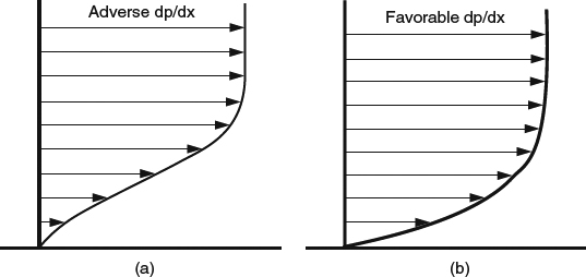
Figure 4.1.5 Effects of pressure gradient on 2D laminar-boundary-layer velocity profiles. (a) Adverse (positive) pressure gradient. (b) Favorable (negative) pressure gradient

In Section 3.6, we discussed the general effects of viscosity and used a notional boundary-layer velocity profile as an example in Figure 3.6.2c. There we noted that the negative second derivative ∂²u/∂y² corresponds to a negative shear-stress gradient ∂τ/∂y, which constitutes a net viscous force on fluid parcels tending to slow the parcels down. The boundary conditions on ∂u/∂y require that every boundary-layer velocity profile have at least one region of negative ∂²u/∂y². And in fact, in the usual situation in most boundary-layer flows, negative ∂²u/∂y² and negative ∂τ/∂y dominate, with the result that fluid parcels in the boundary layer slow down, and the boundary layer grows thicker as it flows along. Of course net viscous forces are not the only thing affecting this boundary-layer growth; the pressure gradient also plays a role. An adverse pressure gradient tends to slow fluid parcels down and hasten the growth the boundary layer, while a favorable pressure gradient tends to slow the growth down and can even reverse it. In Section 4.2.2, we'll see how these effects are quantified in terms of the integrated momentum balance.

The tendency toward positive boundary-layer growth is usually quite pronounced. A boundary layer starting at a stagnation point as in Figure 4.1.1a starts with nonzero thickness, and it is not uncommon for the thickness to grow by a couple orders of magnitude over the length of a body. Streamlined bodies usually have regions of adverse pressure gradient over their aft portions that contribute strongly to the overall boundary-layer growth.

The general tendency of viscous forces to slow fluid parcels down in the boundary layer has an important exception, and that is at the bottom of a boundary layer in an adverse pressure gradient. Note that the velocity profile in the adverse pressure gradient in Figure 4.1.5a has a positive second derivative ∂²u/∂y² close to the wall and a negative second derivative farther out, with an inflection point in between. When we get to the quantitative theory, our discussion in connection with Equation 4.2.7 will explain why this is, but for now the important point is that positive ∂²u/∂y² at the bottom of the boundary layer corresponds to a positive shear-stress gradient ∂τ/∂y, which constitutes a net viscous force on fluid parcels pushing them along in the flow direction rather than impeding them. This “favorable” viscous force is the main mechanism by which the flow at the bottom of the boundary layer resists being slowed in an adverse pressure gradient and thus resists separation, which we'll discuss further in Section 4.1.4.

A boundary layer flow must obey conservation of momentum, both locally and in an integrated sense, something we'll discuss in detail in Section 4.2.2. One result of this is that a boundary layer maintains a “memory” of what it was subjected to upstream, and this memory typically persists over some distance downstream. As an example, consider two turbulent boundary-layer flows, A and B, that are subjected to the same outer flow and differ only in that flow B is subjected to a short patch of surface roughness near the upstream end, that is not present in flow A. For reasons we'll discuss in Section 6.1.8, the roughness in flow B will increase the skin friction locally and thicken the boundary layer, relative to flow A. Conservation of momentum requires that the additional boundary-layer thickness in flow B persists downstream for some distance, but not forever. Downstream of the roughness patch, the skin friction in flow B will be lower than that in flow A because of the increased boundary-layer thickness. The boundary layer thickness in flow B will therefore grow more slowly and asymptotically settle back toward the thickness in flow A. Thus when a boundary-layer flow is perturbed in some way, it “remembers” the perturbation and then gradually “forgets.” We'll see a computational example that illustrates this effect in Figure 6.2.4 in connection with a more detailed discussion of surface roughness.

Note that although the idea of “memory” is applicable in boundary-layer flow, “premonition” is not. In attached boundary-layer flow, “influence” is heavily skewed in the downstream direction, that is, flow conditions at one location along the surface strongly influence what happens downstream but have only very weak influence upstream. In Sections 4.2.1 and 4.2.2, we'll see that in the idealized theory for both 2D and 3D flows the direct upstream influence is predicted to be zero.

In 3D boundary layers, the velocity profile takes on an additional dimension, becoming a two-component vector function. An instructive way of visualizing a 3D velocity profile is to resolve it into components parallel and perpendicular to the outer flow, as shown in Figure 4.1.6. The component in the direction of the outer flow at the local boundary-layer edge is called the streamwise profile, and it looks qualitatively like the velocity profile in a 2D boundary layer, as in Figures 4.1.4 and 4.1.5. The component in the direction perpendicular to the local outer flow is called the cross-flow profile and is different from the streamwise profile in several ways. First, the cross-flow velocity goes to zero by definition at the boundary-layer edge. Second, cross-flow profiles are of different types depending on what “drives” them. If the wall is in motion so as to provide a shearing action in the cross-flow direction, as for example, on a propeller spinner, the cross-flow profile appears as in Figure 4.1.7a and is said to be shear-driven. If the wall is stationary, the cross-flow velocity must go to zero there, and the cross-flow profiles appear as in Figure 4.1.7b,c. Cross-flow of this type is said to be pressure driven, because a pressure gradient in the cross-flow direction is required to set it in motion. And, of course, it is possible for cross-flow to be shear driven and pressure driven simultaneously.

Given the essentially inviscid momentum balance that pertains in the outer flow, a pressure gradient in the cross-flow direction requires outer-flow streamline curvature in the cross-flow direction. So pressure-driven cross flow is always associated with situations in which there is outer-flow streamline curvature in the cross-flow direction. Because the cross-flow direction is parallel to the local body surface, “curvature in the cross-flow direction” refers to the curvature of the streamline as viewed in the local tangent plane of the body surface, as distinct from the part of the curvature that is due to the curvature of the surface itself. We'll explore what this entails in greater detail when we address the theory in Section 4.2.1. The simple way to think of it is that it is the “lateral” component of the outer-flow streamline curvature as seen in a local “plan view” that is associated with pressure-driven cross flow in a 3D boundary layer.

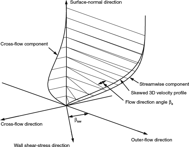
Figure 4.1.6 Isometric view of a 3D velocity profile and its resolution into streamwise and cross-flow components

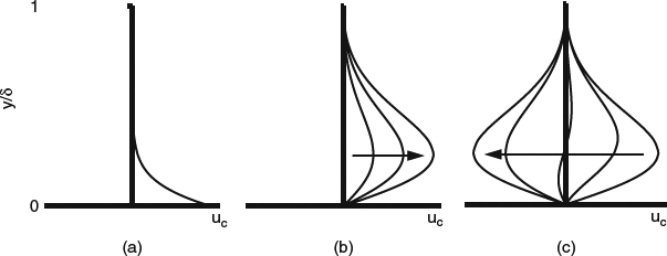
Figure 4.1.7 Profiles of cross-flow velocity u_c in a 3D boundary layer. (a) Shear-driven cross flow produced by motion of the wall. (b) Pressure-driven cross flow increasing. (c) Pressure-driven cross-flow profiles reversing, including one profile of the cross-over type

The effect of the cross-flow pressure gradient on the flow is similar in some ways to the effect of a streamwise pressure gradient that we discussed above in connection with 2D flow in Figure 4.1.5. Like a streamwise pressure gradient, the cross-flow pressure gradient tends to have nearly the same strength regardless of depth in the boundary layer, and it has stronger effects on velocity gradients in the low-velocity fluid deep in the boundary layer than it does in the outer flow. These effects can take the form of rapid changes in flow direction, as, for example, when a boundary layer with little cross-flow flows into a region with a strong cross-flow pressure gradient. In this situation the cross-flow rapidly increases, as in Figure 4.1.7b, and the streamline curvature deep in the boundary layer is much greater than in the outer flow.

Just as we saw in 2D, these effects of pressure gradient in 3D are resisted by viscosity. As we saw for a 2D boundary layer, the tendency of an adverse pressure gradient to slow the flow is resisted by viscous forces produced by the positive second derivative of the velocity profile close to the wall (see Figure 4.1.5a). In a 3D boundary layer with a cross-flow pressure gradient, the tendency of the cross-flow to increase as in Figure 4.1.7b is resisted by viscous forces produced by the negative second derivative of the cross-flow profile typically spanning a region starting at the wall and including the peak of the cross-flow profile. The growth of the cross-flow profile often stops when these two tendencies come into equilibrium.

Of course, inertia also plays a role in the evolution of the cross-flow profile. If the cross-flow pressure gradient disappears, the cross-flow profile lags behind and persists for some distance downstream. If the cross-flow pressure gradient reverses sign, the cross-flow profile reverses first at the bottom of the boundary layer and goes through an intermediate stage with a profile of the cross-over type illustrated in Figure 4.1.7c. Because it is a transient state accompanying a reversal in sign, the cross-flow velocity magnitudes associated with a cross-over profile tend to be small.

The distribution of flow direction in the boundary layer can be expressed in terms of a direction profile, measured by the flow angle β_s relative to the outer-flow direction. The direction profile consistent with a 3D velocity profile like that of Figure 4.1.6 is shown in Figure 4.1.8. In the limit as y approaches zero, this flow direction is the same as the direction of the shear stress at the wall, β_sw, as indicated in Figure 4.1.6.

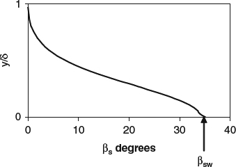
Figure 4.1.8 The direction profile in a 3D boundary layer, in terms of βs, the flow angle relative to that at the edge

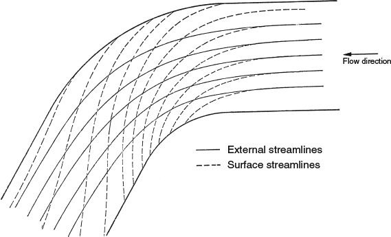
Figure 4.1.9 Skin-friction lines and outer-flow streamlines in a 3D turbulent boundary layer on a flat wall of a curved duct of rectangular cross-section, plotted from measurements by Vermeulen (1971)

Curves constructed parallel to the wall-shear-stress direction are called skin-friction lines, or limiting streamlines, or even wall streamlines, though this last term is misleading, because the velocity at a stationary wall is zero, and no real streamline can be defined. Figure 4.1.9 shows skin-friction lines and outer-flow streamlines in a 3D turbulent boundary layer on a flat wall of a curved duct of rectangular cross-section. The turning of the outer flow is accompanied by a radial pressure gradient that forces the flow deep in the boundary layer to turn inward much more strongly than the outer flow does, as we would expect based on Figure 4.1.6.

The presence of cross flow in a 3D boundary layer often significantly affects the momentum transport and thus the development of the flow compared with what it would be in a 2D boundary layer subjected to the same streamwise pressure distribution. In a 2D boundary layer, the streamwise momentum deficit is convected in only one direction: It comes from upstream and is carried downstream. In a 3D boundary layer, convection is in the direction of the local flow, which varies through the boundary layer, and cross-flow thus plays a direct role in the development of the flow, by transporting momentum “laterally.” Convergence or divergence of the flow in the boundary layer also plays an important role. Figure 4.1.10 illustrates what convergence and divergence look like in cross-flow profiles at locations that are a short distance apart in the cross-flow direction. Note that convergence and divergence don't require a change in sign of the cross-flow velocity, just an increase or decrease. The cross-flow gradient associated with convergence or divergence affects the velocity component normal to the wall through continuity, and thus affects momentum transport indirectly.

The cross-flow gradient also transports mass, which can alter the displacement effect of the boundary layer, as we'll see in Section 4.1.3. And the additional degree of freedom in 3D boundary-layer flowfields opens up the possibilities regarding how the flow can separate from the surface, as we'll see in Section 4.1.4.

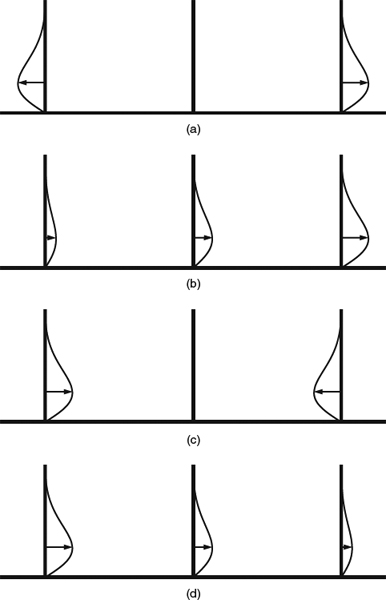
Figure 4.1.10 Examples of cross-flow convergence and divergence. (a) Divergence to either side of a location with zero cross flow. (b) Divergence in cross-flow all of one sign. (c) Convergence to either side of a location with zero cross-flow. (d) Convergence in cross-flow all of one sign

The oil-flow-visualization technique is often used in wind-tunnel testing to visualize the skin-friction lines. Oil is applied to the model surface, and the shear stress drags it along, forming streaks in the direction of the shear-stress lines. The streaky pattern can be made visible by pigment in the oil or by fluorescent dye illuminated by ultraviolet light. Figure 4.1.11 is an example of a fluorescent-oil-flow photo of a swept wing in a wind tunnel. (We'll discuss the specifics of swept-wing boundary layers in Section 8.6.2.) In general, such photos are useful for diagnosing 3D boundary-layer separation patterns, which we'll discuss in detail in Sections 4.1.4, 5.2.2, and 5.2.3. It can also give an indication of the kind of cross-flow convergence or divergence we discussed above.

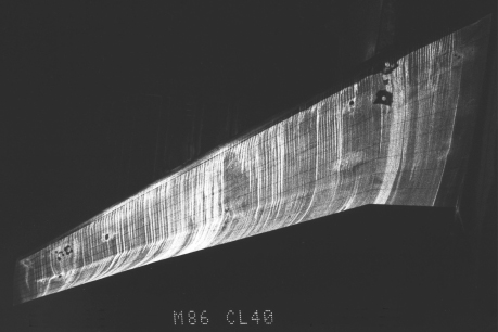
Figure 4.1.11 Fluorescent oil-flow photo of a swept wing in a wind tunnel

As useful as it is, however, oil-flow visualization has a downside: The streaks can give the misleading impression that they represent the general flow direction over the surface. We should always keep in mind when looking at oil-flow pictures that the streaks represent only the surface-shear-stress direction and that the flow direction can be very different only a very short distance above the surface, as indicated by the direction profile Figure 4.1.8. The change in direction above the surface can be especially rapid in a turbulent boundary layer in a strong pressure gradient, as, for example, near the trailing edge of the wing in Figure 4.1.11. The general flow over the surface there doesn't turn outboard nearly as strongly as the oil streaks indicate. The exaggerated turning of the streaks in oil-flow pictures often leads observers to overestimate the importance of “spanwise flow” in swept-wing boundary layers, something we'll discuss further in Section 8.6.2.

4.1.3 Boundary-Layer Displacement Effect

Flow separation like that depicted in Figure 4.1.2b obviously alters the effective shape of the body as seen by the outer flow. What is less obvious is that even an attached boundary layer has a displacement effect, though it tends to be much more subtle than the effect of separation.

We've seen how the no-slip condition and viscous diffusion act in combination to slow the flow in the boundary layer, compared with a corresponding inviscid flow. It follows from the reduced velocity that streamtubes within the boundary layer are thicker than they would have been in the inviscid flow. As a result, the flow outside the boundary layer is displaced outward, away from the body, relative to what would happen in the inviscid case. The effect of this attached-flow displacement effect on the outer flow varies widely depending on how sensitive the outer flow is to small changes in the effective shape of the body. For example, boundary-layer displacement can have dramatic effects on airfoil pressure distributions in transonic flow, as we'll see in Section 7.4.8. But even when the effect on the surface pressures is subtle, it can make a significant contribution to the viscous drag of a body. We'll look at this contribution to pressure drag further in general in Sections 6.1.3 and 6.1.5, and specifically in the case of airfoils in Section 7.4.2.

Note that we just described the displacement effect as the displacement of the outer flow relative to the ideal inviscid flow that would adhere to the contour of the body. In the viscous case, the displaced outer flow acts like a fictitious inviscid flow around a body whose contour has been displaced outward by some amount. In the theory, this fictitious inviscid flow is called the equivalent inviscid flow. Outside the boundary layer and viscous wake, the equivalent inviscid flow is the same as the actual outer flow, while in the region occupied by the boundary layer in the real flow, it is an inviscid extrapolation of the outer flow.

The most widely familiar measure of the displacement effect is the displacement thickness, δ*, which varies along the surface, mostly increasing in the flow direction, and reflects how far outward the boundary layer has displaced the effective surface as seen by the equivalent inviscid flow. We'll look at using δ* as way to quantify the effect in Section 4.2.3. In 2D flow, the slowing of the flow in the boundary layer generally results in positive δ*, except in cases with strong cooling at the surface, which can produce a sink effect that overrides the slowing effect.

So, if we shift the body contour outward by the distance δ,* we define a new body, the equivalent body seen by the equivalent inviscid flow. But what determines how large δ* must be to have the required effect? First, the equivalent body surface must meet the flow-tangency requirement, that is, it must be a stream surface of the equivalent inviscid flow. But this requirement by itself is not sufficient to determine a unique value of δ* because the equivalent inviscid flow has an infinity of stream surfaces where a solid surface could be placed, all presumably having the same effect on the remainder of the outer flow. How do we choose which of these possible stream surfaces is the “right” one for our purposes? To illustrate the problem, Figure 4.1.12 shows schematically the streamlines of the equivalent inviscid flow around a 2D airfoil-like body. It is clear that there is only one streamline that splits at a closed “leading edge” and becomes two streamlines that pass the body on opposite sides (shown as heavier lines than the others). If we choose streamlines farther from the body than these, the equivalent body must extend upstream to infinity, and if we choose streamlines closer than these, the equivalent body must spew mass out of part of its leading edge. These other options would work, in principle, but they'd be inconvenient, to say the least.

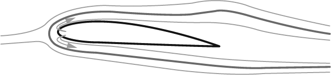
Figure 4.1.12 Schematic of streamlines of the equivalent inviscid flow around a 2D airfoil-like body. Only the streamline indicated by the heavier curve forms an equivalent body that is closed at the front and is therefore the preferred streamline to define the displacement thickness of the boundary layer of the actual viscous flow. Distances from the body are exaggerated for clarity

The preferred equivalent-outer-flow streamline forms a blunt nose that mimics the shape of the body. The displacement thickness is therefore defined and nonzero at the stagnation point. We'll look at how this works in more detail in Section 4.2.3.

Thus the preferred choice of equivalent-outer-flow streamline to define δ* is the one for which the equivalent inviscid flow has no mass-flow missing (because the equivalent body extends upstream to infinity) and has no extra mass-flow spewing from its leading edge. With this definition of δ*, the equivalent inviscid flow between the δ* surface and any point outside the boundary layer has the same mass flux as the actual viscous flow does between the wall and the same point. In Section 4.2.3, this will be our basis for defining δ* in 2D as a function of the local velocity profile.

Now note that the equivalent-inviscid-flow streamlines defining δ* behind the body “neck down” somewhat, but never close off. This reflects the fact that the viscous wake downstream of the body always carries some velocity deficit and therefore retains some displacement effect.

The simple mass-flux argument we made using Figure 4.1.12 to define δ* in 2D flow doesn't apply in general in 3D. In 3D flows, cross flow can have a major influence on the displacement effect and can decouple it from the local streamwise velocity profile, so that while 2D δ* can be inferred from the local velocity profile, 3D δ* cannot. Cross-flow convergence can “pile up” fluid in the boundary layer and increase the displacement thickness. Likewise, cross-flow divergence carries fluid away laterally and decreases the displacement thickness. The general slowing of the flow in the boundary layer still tends to produce mostly positive δ*, in the absence of strong cooling. In limited regions of strong cross-flow divergence, however, δ* can be negative. In this situation, the boundary-layer fluid that has been carried away laterally by the divergence must be replaced by the outer flow, and it then appears to the outer flow as if the effective body contour has been locally carved away rather than thickened. Of course, the fluid that is carried away from a region of divergence has to go somewhere, and as a result, regions of negative δ* are always flanked by areas of unusually large positive δ*.

The general interpretation of the δ* surface as an effective solid-wall boundary for an equivalent inviscid flow is a useful mental model, but it is sometimes leads to misunderstanding. The δ* surface represents an effective solid wall only for the flow situation that produced the boundary-layer flow with that particular distribution of δ*. In a different flow situation, say because some part of the body geometry elsewhere changes, the entire flow will change, including the δ* surface, and the flow will not respond as if the original δ* surface were a solid surface.

A misunderstanding in this regard has arisen in connection with wind-tunnel half-model testing. This is the testing of a model of half of an airplane mounted on a solid wind-tunnel wall that is supposed to enforce a symmetry-plane boundary condition, so that the flow is equivalent to symmetrical flow around a full model. In the idealized situation, the nominal symmetry plane of the model coincides with a flat wall of the tunnel, as illustrated in Figure 4.1.13a. In inviscid flow, this arrangement provides perfect simulation of the full-model flow. In a real viscous flow, however, the symmetry-plane boundary condition is rendered imperfect by the boundary layer on the tunnel wall. An idea that is intuitively appealing, and that has frequently been put into practice, is that using a “standoff” spacer to move the model off the wall by a distance equal to δ* of the empty-tunnel boundary layer, as illustrated in Figure 4.1.13b, is the right thing to do on physical grounds, since the δ* surface should be the effective location of the solid wall. But this is erroneous physical reasoning. Although the empty-tunnel δ* represents an effective solid-wall boundary condition for the empty tunnel, it doesn't do so in the presence of flow changes introduced by the model. A computational fluid dynamics (CFD) study (Milholen, Chokani, and McGhee, 1996) looked at a range of standoff heights and several strategies for controlling the tunnel-wall boundary layer. The results indicated that the best simulation of full-model conditions should be achieved when no model offset is used, and the wall boundary layer is thinned by tangential jet blowing just upstream of the model. (The authors did not calculate the case of zero height, but extrapolation of their results indicates that it would be best.)

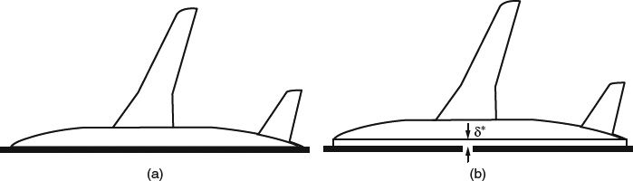
Figure 4.1.13 Schematic illustrations of a half model mounted on the wall of a wind tunnel. (a) Nominal symmetry plane of the model coincides with a flat, solid wall of the tunnel. (b) A spacer is used such that the nominal symmetry plane of the model is spaced away from the wall at the empty-tunnel δ* surface, which is often erroneously thought to provide a better reflection plane

4.1.4 Separation from a Smooth Wall

So far, we've seen what 2D separation from a smooth wall looks like topologically in Figure 4.1.2b. Now we'll look at the physics of separation. First, what determines whether a boundary layer separates, and if so, where it separates?

Whether the boundary layer separates or stays attached is determined by what happens to the low-velocity fluid at the bottom of the boundary layer. In an attached-flow region, all of the fluid is moving in the general direction of the outer flow, which, if we take the outer-flow direction to be positive, means that the velocity in the entire boundary layer is positive, except at the wall itself, where it must go to zero. This, of course, requires the slope of the velocity profile to be positive at the wall. Just downstream of separation, there must be a region of reverse flow next to the wall, which requires a negative slope of the velocity profile at the wall. So going from attached flow to separated flow requires a decrease in the slope of the velocity profile at the wall from positive to negative, and the slope must go through zero at the separation point. This sequence is easiest to see and understand in the case of laminar flow, as sketched in Figure 4.1.14a.

As we saw in Section 4.1.2, an attached boundary layer usually thickens as it flows downstream, as viscosity and the no-slip condition act in concert to decelerate the flow. The slope of the velocity profile at the wall thus naturally tends to decrease gradually. But viscosity and the no-slip condition are not sufficient to make the slope go through zero and become negative as in Figure 4.1.14a. For that, an adverse pressure gradient (rising pressure) is also required. How do we know that an adverse pressure gradient is needed? Note that for the negative velocity slope at the wall to appear, there must be a region in which the velocity profile is concave “forward” (positive ∂²u/∂y²) somewhere within the boundary layer. When such a region appears, it generally appears first adjacent to the wall, as it does in the sequence sketched in Figure 4.1.14a. In a laminar boundary layer, or at the bottom of a turbulent boundary layer, positive ∂²u/∂y² means that the shear stress gradient ∂τ/∂y is also positive. In our discussion of the theory in connection with Equation 4.2.7, we'll establish that positive ∂τ/∂y at the wall requires an adverse pressure gradient.

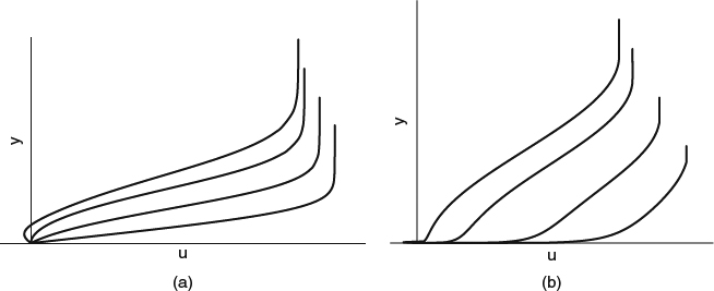
Figure 4.1.14 Progression of velocity profiles in a 2D boundary layer going through separation. (a) Laminar flow. (b) Turbulent flow

So it takes an adverse pressure gradient to cause separation of the boundary layer. But an adverse pressure gradient also activates a mechanism by which the boundary layer tends to resist separation, enabling it to remain attached at least for some distance into the region of adverse pressure gradient. As we saw above, an adverse pressure gradient results in a positive ∂τ/∂y close to the wall. Of course, ∂τ/∂y is the net viscous force on a fluid parcel (see the discussion in Section 3.6 and the flow examples in Figure 3.6.2), and positive ∂τ/∂y thus constitutes a net viscous force opposing the pressure gradient. In effect, the fluid at the bottom of the boundary layer experiences a “favorable” viscous force. One way to think of it is to imagine the higher-velocity fluid farther from the surface acting through the viscous stress to drag the lower-velocity fluid along, fighting against the pressure gradient that is trying to slow the fluid down.

Boundary-layer separation thus involves a tug-of-war between the adverse pressure gradient and an opposing viscous force. At any given station along a surface subjected to an adverse pressure gradient, the favorable viscous force will generally be overmatched, and you'll see the pressure gradient winning the tug-of war, slowing the fluid near the wall, and reducing the velocity slope at the wall. How far the boundary layer will be able to persevere into the adverse pressure gradient before it separates depends on the rate at which the pressure gradient wins and the velocity slope at the wall decreases. Although the favorable viscous force is generally overmatched locally, its presence is vital. As we'll see below, if it weren't for the favorable viscous force, a boundary layer starting into an adverse pressure gradient would separate immediately. With the favorable viscous force, the rate of approach to separation is finite, and the distance from the onset of the adverse gradient to separation is nonzero. Until the slope of the velocity profile at the wall is brought to zero, the boundary layer remains attached, just as the corresponding inviscid flow would under the same conditions. Separation occurs only when the adverse pressure gradient has acted over a long enough distance to produce reversal of the velocity profile. How long that distance is depends on a number of factors that we'll discuss in Section 7.4.3 in connection with the maximum lift of airfoils.

Thus we've established viscosity as a source of resistance to separation, which seems contradictory because we also tend to think of viscosity as one of the main causes of separation. Without viscosity and the no-slip condition, a flow can remain attached over the entire length of a body, surviving the adverse pressure gradient all the way to an aft stagnation point without separating. But with viscosity and the no-slip condition, there must be a boundary layer with zero velocity at the surface, which introduces the possibility of separation when the flow encounters an adverse pressure gradient. So separation is a possibility only because viscosity and the no-slip condition have introduced a viscous velocity profile. On the other hand, once an adverse pressure gradient sets in, viscosity is the only source of resistance to separation. If you turned off the viscous stresses at the start of the adverse pressure gradient (i.e., switched to Euler equations with the incoming boundary-layer velocity profile as the upstream boundary condition), the flow would separate immediately. The flow near the wall, with near-zero velocity, has near-zero capacity to proceed into a pressure rise without the favorable viscous effect that we discussed above. So viscosity is both an enabler of separation and a source of resistance to separation. The key to this seeming contradiction is that the net viscous force is just ∂τ/∂y, which is negative in most of the boundary-layer flowfield, slowing the fluid parcels down. Then at the start of an adverse pressure gradient, ∂τ/∂y switches to positive at the bottom of the boundary layer and helps that part of the flow overcome the pressure gradient, at least for a while. This favorable viscous effect acts only in the bottom part of the boundary layer in an adverse pressure gradient, while viscosity everywhere else has an adverse effect.

A laminar boundary layer cannot withstand much of a pressure rise without separating (see White, 1991, section 4-2), because the favorable viscous force that resists separation comes only from molecular shear stress, which tends to be small. The amount of pressure rise that can be withstood by a turbulent boundary layer, on the other hand, is much greater, because the favorable net viscous force is much stronger. At first glance it's tempting to think that this is simply because the eddy viscosity and the turbulent shear stress are so much larger than their molecular counterparts (we discussed turbulent shear stress and the eddy viscosity in Section 3.7), but the correct explanation is more complicated. If the eddy viscosity were simply larger, but uniform throughout the boundary layer, we would have the equivalent of a laminar boundary layer at a lower Reynolds number, and separation resistance would be no greater. The key is that a turbulent boundary layer has a thin sublayer next to the wall, in which the eddy viscosity is effectively zero, and that the eddy viscosity increases rapidly with distance from the wall outside this sublayer. We'll look in some detail at the physics of the sublayer and the role it plays in the greater separation resistance of turbulent boundary layers in Section 4.4.2.

In the regions of pressure rise that frequently occur in practical flows around bodies, a turbulent boundary layer is usually required if separation is to be avoided. Streamlined bodies, which we'll discuss in greater detail in Sections 5.2 and 6.1.6, must generally have a region of pressure rise at the rear, often referred to as a pressure recovery, and turbulent flow is generally required to prevent premature separation there. Even so-called laminar-flow airfoils (Section 7.4.6) are generally designed to have laminar flow over only part of the airfoil chord, with the boundary layer transitioning to turbulent before it tries to proceed too far into the region of the pressure recovery.

Avoiding premature separation is important in many applications. In external flows, there are the pressure recoveries on airfoils and other streamlined bodies. In internal flows, ducts that serve to provide pressure recovery are often called diffusers, and they are important in propulsion inlets, wind tunnels, and many other flow systems. In such applications, the designer's objective is often to maximize the recovery that can be achieved in a given length or to minimize the length for a given recovery. In this regard, the performance of a flow device with a pressure recovery is strongly dependent on the details of the pressure distribution in the recovery region. We'll consider this issue in some detail in connection with the maximum lift of airfoils in Sections 7.4.3 and 7.4.4, and in Section 4.5 we'll look at general strategies for delaying or preventing separation.

Now let's look further into what happens as a 2D flow approaches separation. Velocity profiles of flows going through separation are illustrated in Figure 4.1.14, for laminar flow and turbulent flow. We've already noted that the basic flowfield topology requires that downstream of separation there be reverse flow close to the wall, which requires negative ∂u/∂y at the wall, and that the boundary between attached flow and separated flow is where ∂u/∂y at the wall goes through zero. The surface shear stress and the skin-friction coefficient are therefore zero at the separation point, but we must remember that this applies only in 2D flow.

Where ∂u/∂y goes through zero at the separation point is easy to see in plots of laminar velocity profiles, as in Figure 4.1.14a. In plots of mean (time-averaged) velocity profiles in turbulent flow, separation doesn't stand out so clearly. A turbulent velocity profile at separation can give the appearance of still having a large positive ∂u/∂y at the wall, because ∂u/∂y can drop to zero over a very short distance from the wall, not visible on the scale of a plot like Figure 4.1.14b. This is related to the existence of the thin sublayer we mentioned above, and which we'll discuss in detail in Section 4.4.2. And there are other ways in which the turbulent case is complicated. Turbulent separation is of course unsteady on length and time scales related to the boundary-layer turbulence, and often on longer time scales as well. This means that turbulent separation is marked by two thresholds: the first appearance of intermittent reverse flow, followed downstream by reversal of the mean flow. The special complexities associated with separation in turbulent flow are discussed in detail by Simpson (1989).

Separation in 3D flow is also driven by the pressure gradient, but not just by its streamwise component. We can still think of separation as involving the reversal of one component of the velocity close to the wall, but it needn't be the outer-flow-streamwise component. And a line along which separation takes place, which we'll call a separation line, needn't be perpendicular to the local outer flow, as it would be in 2D.

In some situations, in fact, a separation line can be closer to parallel to the outer flow than to perpendicular. In such cases the separation is sometimes called a “cross-flow separation” (see Hirsch and Cebeci, 1977, for example), because it can be accompanied by reversal of the cross-flow profile. This is unfortunate terminology because it implies that cross-flow reversal defines the separation. Actually, cross-flow reversal occurs in many situations not even remotely associated with separation, and even in cases of so-called cross-flow separation, it isn't the cross-flow reversal that defines the separation location. Cross-flow separations are just situations in which the cross-flow reversal happens to occur very close to the actual separation location.

So separation in 3D is not generally defined by a reversal of either the streamwise or the cross-flow velocity profile, or by zero C_f in either the streamwise or the cross-flow direction. But then what is it defined by? Separation in general involves some flow leaving the surface and forming a shear layer that is at least somewhat “separated” from the surface, and we'll look at some of the separated-flow structures that arise in 3D in Section 5.2.2. But separation should also have a telltale signature on the surface. In 2D, that signature is zero C_f. What is the corresponding signature in 3D?

In Section 4.1.1, we noted that a line of separation on the surface divides the surface into regions from which the flow just off the surface is converging from different directions. In the limit as we approach the wall, the direction of the flow just off the surface defines the direction of the surface shear stress, or the direction of the skin friction lines, which we defined in Section 4.1.2. A 3D separation line is thus a skin-friction line flanked by other skin-friction lines converging toward it from different directions, as in Figure 4.1.15. Although the magnitude of C_f is not zero, the component of C_f perpendicular to the separation line is zero, just as is was in 2D. But zero perpendicular C_f isn't sufficient as a definition of the separation line because it is satisfied on every other skin-friction line as well. And the fact that other skin-friction lines converge toward it doesn't suffice either. So we must look at other aspects of the direction field on the surface to see what it is that makes the separation line different.

Looking at the global pattern on the surface, we see that what distinguishes a 3D separation line is the longer term “history” of the skin-friction lines converging toward it: The skin-friction lines converging toward the separation line from opposite sides “arrive” from locations on the surface that are far apart. Thus I propose as a working definition of a separation line that skin-friction lines converging toward it from opposite sides have different regions of origin.

This isn't a mathematically rigorous definition, but we can use a math-like argument to elaborate on what it means. Consider two points close together on the surface, both of them on the same side of a separation line, and consider the skin-friction lines that “arrive” at these points from “upstream,” as illustrated in Figure 4.1.16a. The path followed by each of these skin-friction lines can be thought of as being a kind of mathematical function in which the points on the surface map into the surface streamlines arriving at the points. This function can be said to be continuous in the sense that skin-friction lines 1 and 2 can be made arbitrarily close together anywhere along their length if we make points 1 and 2 sufficiently close together. In a strict mathematical sense, this kind of continuity also applies to two points on opposite sides of a separation line, as sketched in Figure 4.1.16b, but there is a practical difference. Crossing the separation line, the rate of change of the “function” is much larger than it is elsewhere, as you can see qualitatively by comparing parts (a) and (b) of Figure 4.1.16. Practically speaking, the separation line is a near-discontinuity in the region of origin of the skin-friction lines, which is the most precise way of stating my proposed working definition of a separation line in 3D.

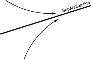
Figure 4.1.15 Local view of a 3D separation line with other skin-friction lines converging toward it

A swept wing is one major application for which it is important to remember that separation in 3D is not generally characterized by zero C_f. We'll look at swept-wing separation patterns and at how the region-of-origin definition of separation applies to them in Sections 5.2.3.2 and 8.6.2.

The region-of-origin way of defining 3D separation leads naturally into a discussion of the distinction between the two major types of separation lines illustrated in Figure 4.1.17. The separation line in Figure 4.1.17a divides a region where the boundary layer is fed by “clean” outer flow originating upstream of the body, from a region within a “closed” separation bubble. This is often referred to as a closed separation. If the bubble's footprint on the surface ends at a sharp trailing edge, as on a wing, the separation line can be an actual discontinuity in the region of origin of the skin-friction lines. The other major type is the separation line in Figure 4.1.17b, which is flanked on both sides by boundary layers fed by “clean” outer flow. This type is often called an open separation. Note that although the open separation doesn't divide regions of the surface fed by different kinds of flow, it is still a near-discontinuity in the region of origin of the skin-friction lines.

Although Figure 4.1.17 is a good representation of the general distinction between open and closed separation, there is one detail that is not quite right. It shows adjacent skin-friction lines joining the separation line tangentially but firmly, where skin-friction lines in actual flows do so only asymptotically. This is an issue we'll discuss further in Section 4.2.5.

The idea of pressure recovery that we discussed in connection with 2D separation is also relevant to 3D separation, but in 3D it is not just the streamwise component of the pressure gradient that is important. 3D effects can either increase or reduce the amount of recovery that can be withstood without premature separation. To take one important example, wing sweep generally reduces the amount of pressure recovery that the boundary layer can withstand, in absolute terms. We'll look at CFD calculations illustrating this effect in Section 8.6.2.

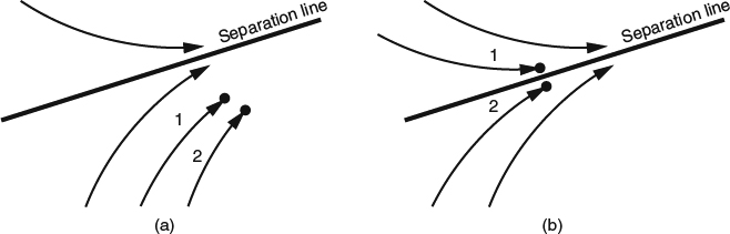
Figure 4.1.16 Illustrations of the concept of the region of origin of skin-friction lines, as applied to two typical points on the surface. (a) Two points to one side of a separation line. (b) Two points flanking a separation line

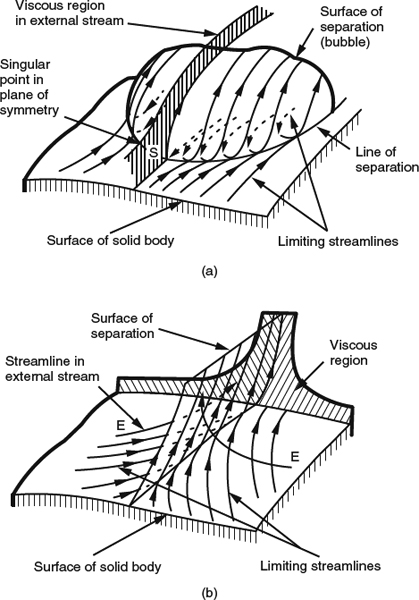
Figure 4.1.17 Illustrations of the two major types of 3D separation lines. (a) Closed type (“bubble”). After Maskell, (1955). From Peake and Tobak, (1980). Published by NASA. (b) Open type (“free shear layer”). After Maskell (1955). From Peake and Tobak (1980), published by NASA

4.2 Boundary-Layer Theory

The idea of dividing the flow around a body, for theoretical purposes, into an outer inviscid flow and an inner viscous flow, both governed by simplified equations, was introduced by Prandtl (1904) and has been extensively developed in the years since. For decades, this approach provided the only means for making quantitative predictions of viscous flows at high Reynolds numbers. Even in the 1970s and 1980s, when CFD predictions of transonic inviscid flows became practical, calculations based on boundary-layer theory provided the only economical means for accounting for viscous effects. In Chapter 10, we'll discuss some of the methods by which coupled CFD solutions are obtained for inner and outer flow regions. In this section, we'll concentrate on the theory and what we can learn from it about the flow in the boundary layer itself.

4.2.1 The Boundary-Layer Equations

Prandtl's, 1904 derivation of the equations of motion for the flow in the boundary layer was based on physical reasoning and an order-of-magnitude analysis applied to the 2D NS equations. The boundary-layer equations can also be derived by a more formal procedure based on the method of matched asymptotic expansions (Van Dyke, 1964). In this procedure, the flow is divided into overlapping inner and outer regions, and the NS equations are expanded in terms of a small parameter (R^−1/2 for laminar flow). The same boundary-layer equations arrived at by Prandtl arise as the equations governing the first-order solution for the inner-region flow. The equations that arise for the outer-region flow are inviscid, as was also proposed by Prandtl. This is an interesting example of sound physical intuition being reinforced much later by rigorous mathematical analysis. The more rigorous later theory has provided a basis for going beyond the original theory, as, for example, in higher order elaborations of boundary-layer theory, and asymptotic analyses of flows in regions where the first-order boundary-layer approximations break down, for example, at trailing edges of plates and airfoils.

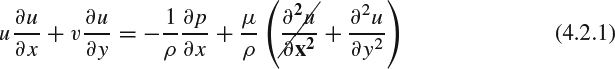
To see how Prandtl's original 2D boundary-layer equations arise and how they relate to the corresponding NS equations, consider the boundary-layer flow developing along the surface of a body as shown in Figure 4.2.1. The flow is described in a curvilinear coordinate system with x along the body surface and y perpendicular to it, but because of the thinness of the boundary layer, we ignore the curvature of the surface and of the coordinate system. The boundary layer (the region in which the effect of viscosity is significant) is assumed to have a small thickness δ(x), and x derivatives of flow quantities are assumed to be much smaller than y derivatives. The 2D NS equations for constant-property, steady, laminar flow are given below. The strikethroughs indicate the terms that were eliminated by Prandtl's order-of-magnitude analysis to yield the boundary-layer equations:

x momentum:

y momentum:

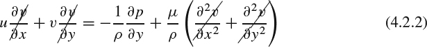
which reduces to

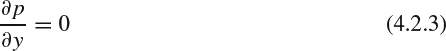
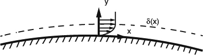
Figure 4.2.1 2D boundary layer developing on the surface of a body, and the coordinate system used in the 2D boundary-layer equations

Continuity:

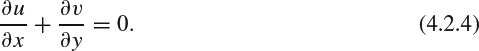
For Reynolds-averaged turbulent flow, we would have to add a Reynolds-stress term to represent turbulent transport in the momentum equation, and then to have a complete set of equations, we would have to incorporate a turbulence model, as discussed in Section 3.7. For compressible flow (variable properties), we would also need to include the thermal energy equation, an equation of state, and an equation defining μ as a function of other fluid properties (usually temperature only). The momentum and continuity equations for incompressible flow will suffice for purposes of this discussion. Note that Equation 4.2.3 stipulates that, according to this set of first-order boundary-layer assumptions, the pressure p is constant in the y direction and is thus effectively a function of x only. The pressure in the x-momentum equation is thus imposed unchanged across the entire thickness of the boundary layer and is, in effect, an environmental condition imposed on the boundary layer from the outside.

So, what does the above simplification accomplish? Remember from Section 3.2 that the NS equations are hyperbolic-elliptic in space, which means that the solution at any one point depends on the solution everywhere else. This, combined with the nonlinearity of the equations, effectively precluded the economical computation of numerical solutions for most purposes, even in 2D, until the 1980s. The boundary-layer equations, on the other hand, are parabolic because all second derivatives with respect to x have been eliminated, which means that they in effect represent an initial-value problem in x. Starting with an initial condition (initial velocity profile) at an initial x station, we can determine the solution in a one-pass marching sequence from upstream to downstream, and the required computational effort is much less than that required for a corresponding NS solution. Economical numerical solutions to the full boundary-layer equations were obtained in the 1960s.

And further simplifications apply in special cases. There are special situations in incompressible laminar flow, which we'll consider in Section 4.3.2, for which the pioneers of boundary-layer theory were able to find similarity transformations that reduce the boundary-layer equations from partial-differential field equations (PDEs) to an ordinary differential equation (ODE), greatly reducing the effort required to generate numerical solutions.

Even in more general situations in which the similarity transformations don't apply, incompressible laminar flows can often be simplified in another way. Equations 4.2.1–4.2.4 can be transformed into a dimensionless form in which the Reynolds number appears only in the definition of the transformed vertical velocity v and not explicitly in the equations themselves (White, 1991, Section 4.2). Thus the dimensionless development of an incompressible laminar boundary layer can be independent of Reynolds number, provided it starts with an initial condition that is consistent with the Reynolds number. A common situation that meets this requirement is when the boundary layer starts at a stagnation point of the 2D outer flow. The 2D stagnation-point boundary layer is one of the similarity situations we alluded to above, and it scales in the right way with Reynolds number so that the development of the rest of the flow downstream will be independent of Reynolds number even if it is nonsimilar. One consequence of this is that incompressible laminar separation depends only on the pressure distribution, not on the Reynolds number, provided the flow starts at a stagnation point.

In Section 4.1.4, we discussed how separation is determined by a tug-of-war between the viscous shear-stress gradient ∂τ/∂y and the pressure gradient dp/dx. So how can separation in laminar flow be independent of Reynolds number? Doesn't a change in Reynolds number change the viscous stress? Well, yes, but the change in boundary-layer thickness compensates for it so that the balance between the shear-stress gradient and the pressure gradient remains the same. To see how this works, consider two flows in which the body shape and the flow quantities ρ and u_∞ are the same, but the viscosity μ is different. At comparable locations in the boundary layers in the two flows (same station on the body, at the half-way point in the boundary-layer thickness, for example), we would have τ ∼ μ, if ∂u/∂y were the same. But ∂u/∂y is not the same. In a laminar boundary layer that displays the kind of global Reynolds-number independence we're talking about, the boundary-layer thickness δ ∼ μ^0.5, so that ∂u/∂y ∼ μ^−0.5, and τ = μ∂u/∂y ∼ μ^0.5. Then taking ∂τ/∂y introduces another factor of μ^−0.5, so that ∂τ/∂y is independent of μ.

The flow around a circular cylinder is a classic example of this kind of behavior in which laminar separation takes place at a fixed location in the pressure distribution, independent of Reynolds number. Assuming ideal potential flow as the outer-flow input (the effect of the separated wake is not accounted for), an early series solution predicted separation at the 108.8° location on the cylinder (see Schlichting, 1979). It has since been realized that the series solution converges poorly near separation, and more recent numerical solutions give separation at 104.5° (see White, 1991).

In the world governed by the parabolic boundary-layer equations, “information” is directly transmitted in the downstream direction but not the upstream direction. If the pressure distribution p(x) imposed on the boundary layer is held fixed, the flow at any one point within the boundary layer depends on, but has no direct influence on, the flow at points upstream, while the flow at one point influences the flow everywhere downstream. Upstream influence can happen only indirectly through interaction with the outer inviscid flow, which would be felt through changes in p(x). There are two important points to note about this. First, the complete asymmetry between the directions (influence travels downstream but not upstream) reflects the fact that the boundary layer is largely a dissipative viscous flow and is therefore irreversible. Second, the absence of direct upstream influence is an idealization resulting from the theoretical assumptions: the neglect of the streamwise viscous diffusion term in the x-momentum Equation 4.2.1 and the assumption that pressure is an imposed environmental condition that doesn't vary with y. These assumptions don't hold exactly in any real flow. But they are good approximations in many situations, and even in many situations in which they are significantly violated locally, the effects of the violation tend to be localized. For example, if a disturbance in the form of a small bump on the surface is introduced into a real boundary-layer flow, it will, of course, have some direct influence on the flow upstream, primarily through its disturbance pressure field, which will vary in y. But its significant upstream influence will be confined to within a few bump lengths or heights of the bump itself, and if the bump is small, it's direct upstream influence will be limited to a short distance. Thus the idea that direct upstream influence in boundary-layer flows is limited, but that downstream influence can be far reaching, is a useful insight. Of course, this applies only to boundary layers that remain thin and attached to the surface. If the boundary layer separates from the surface, its upstream influence through the outer flow becomes much stronger.

While the boundary-layer equations represent an initial-value problem in x, they also require boundary conditions, some of which can vary with x. At the inner boundary, the usual solid-wall no-slip boundary condition is u = v = 0 at y = 0, just as it was for the NS equations. For the normal velocity v, this inner condition is all that we can impose, because the highest order y derivative is ∂v/∂y. The outer boundary conditions on the rest of the solution are a little more complicated. We've already observed that the pressure is effectively one boundary condition imposed on the boundary layer from the outside, but we still must apply a condition to the tangential velocity u. Note that ∂u/∂y should tend toward zero for large y, so that the x-momentum Equation 4.2.1 reduces to the 1D inviscid momentum (Euler) equation:

with the pressure independent of y as stipulated in Equation 4.2.3. Thus for large y, u should tend toward a value u_e (x) that is independent of y and consistent with Equation 4.2.5. We can either impose p(x) as the “outer” boundary condition and let u_e (x) “fall out” as an implicit result of Equation 4.2.5, or we can impose u_e (x) as the boundary condition and use Equation 4.2.5 explicitly to determine a consistent p(x) to impose in Equation 4.2.1. In any case, we will usually use either p(x) or u_e (x) as an outer-flow matching condition, that is, we will require it to match the distribution for some outer inviscid flow. Solving the boundary-layer equations with either p(x) or u_e (x) as an explicit boundary condition is referred to as the direct mode. Solving the equations with a boundary-layer flow variable such as the displacement thickness (which we'll define in Section 4.2.3) or the skin-friction coefficient C_f imposed and allowing p(x) and u_e (x) to “fall out” is referred to as an inverse mode.

The terms in the streamwise momentum Equation 4.2.1 have straightforward physical interpretations easily related to our physical discussion of Section 4.1.2. The two convective-acceleration terms represent the steady-flow part of the Lagrangian acceleration of fluid parcels as they pass through the flowfield, in the manner we discussed in Sections 3.2 and 3.4.6, and the pressure gradient and shear-stress terms represent the internal fluid-stress gradients that provide the acceleration.

Some further discussion of the order-of-magnitude argument is called for here. At first, it might seem surprising that neither of the convective acceleration terms was eliminated in going from the NS equations to the boundary-layer equations. After all, the boundary layer is a thin region, and because v in the boundary-layer coordinate system must be zero at the wall, v will be small everywhere in the boundary layer. So why can't we neglect v∂u/∂y? It turns out that although v is small, v∂u/∂y and u∂u/∂x are of the same order, as Prandtl's order-of-magnitude analysis showed.

To see how this comes about, consider what determines the magnitude of v in a boundary layer. Although v must of course obey a vertical momentum balance, the momentum balance isn't actually operative in determining v, because all of the terms in the y-momentum Equation 4.2.2 are negligible in the boundary-layer version, Equation 4.2.3. Instead, to determine v we must resort to the continuity equation. Integrating the continuity Equation 4.2.4 in the y direction, noting that v = 0 at y = 0, we get

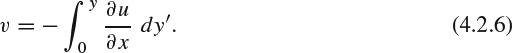
So in boundary-layer theory, the vertical velocity v is of the same order as y∂u/∂x. Furthermore, it is proper to think of v as being primarily a result of the combination of continuity and ∂u/∂x, and to think of the small ∂p/∂y in the vertical momentum balance as adjusting to accommodate the v distribution that continuity imposes.

Now because v is of the same order as y∂u/∂x, we must keep both convective terms in the x-momentum equation. And so even in a boundary-layer flow, u∂u/∂x isn't the only significant contributor to the Lagrangian acceleration. Because of the v∂u/∂x term, the actual Lagrangian acceleration of fluid parcels in a boundary layer is typically considerably smaller, in an absolute-value sense, than u∂u/∂x. Even though v is small, it makes an important contribution to the boundary-layer's streamwise momentum balance.

At the bottom of the boundary layer, the relative importance of the terms in the momentum balance is different from what it is at the edge. We saw above that according to Equation 4.2.5, the momentum balance at the edge of the boundary layer involves only the pressure gradient and the longitudinal acceleration. At the bottom of the boundary layer, the situation is very different, and the gradients of the shear stress and the pressure dominate. In the limit as the wall is approached, the convective terms in the x–momentum Equation 4.2.1 vanish, and the equation reduces to

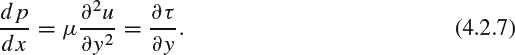
This equation applies only to a very limited region at the bottom of the boundary layer, but it still provides interesting insights. It requires, for example, that in an adverse (positive) pressure gradient ∂²u/∂y² and ∂τ/∂y must be positive at the wall. We looked at the implications of this in the physics of flow separation in Section 4.1.4. Because the second derivative is always negative in the outer part of the layer, this means that the velocity profile of a laminar boundary layer in an adverse pressure gradient must always have an inflection point. We'll see in Section 4.4 that this has implications for the stability of the laminar boundary layer.

The 3D boundary-layer equations are analogous to the 2D Equations 4.2.1–4.2.4, with two velocity components, u and w, parallel to the surface, in place of just u, and an additional component of momentum to be accounted for. The momentum Equation 4.2.1 thus becomes a two-component vector equation, or two equations. And in place of just one coordinate, x, along the surface, we must now have two, x and z. If the body surface has compound curvature, the x-z coordinate system that is laid out in the surface must be curvilinear, and coordinate metrics and curvature terms must be introduced. And it is often convenient to make the coordinate system in the surface nonorthogonal. In this respect, the 3D boundary-layer equations are no different from most implementations of the 3D NS equations, and tensor notation provides the least error prone way to derive equations in curvilinear, nonorthogonal coordinates. For the boundary-layer equations, details can be found in the book by Nash and Patel (1972).

The x-z coordinate system for the 3D boundary-layer equations can be laid out arbitrarily on the body surface. The velocity profiles described in an arbitrary coordinate system can look quite different from the streamwise and cross-flow profiles that we considered earlier. Figure 4.2.2 shows what the velocity profiles of Figure 4.1.6 would look like in an arbitrary boundary-layer coordinate system x_b,z_b.

In some situations, particular choices of coordinate alignment can make life much easier. For example, if a numerical solution is to be generated in a marching sequence, it may be necessary to align one coordinate or the other roughly in the dominant flow direction. Sometimes it may be advantageous to align one of the coordinate families with the streamlines of the outer flow, a choice referred to as streamline coordinates, though this is not often done in practice. Sometimes one coordinate line is aligned with a line along which the initial conditions for the boundary-layer flow are known or can be easily generated as solutions to the plane-of-symmetry boundary-layer equations, simplified versions of the 3D equations that we'll discuss in Section 4.3.4. Examples of this would be to align one coordinate line with a plane of symmetry of a body or the leading-edge attachment line on a swept wing, as shown in Figure 4.2.3.

In Section 4.1.2, we discussed in physical terms how the presence of cross flow affects the momentum balance in a 3D boundary layer, and how cross flow is related to the pressure gradient in the cross-flow direction. We also saw how a pressure gradient in the cross-flow direction requires outer-flow streamline curvature in the cross-flow direction. What this means is illustrated in Figure 4.2.4. The outer-flow streamline projected onto the body surface forms a 3D space curve that at any given point has a unit tangent vector t. When the curvature dt/ds (the of change of t along the curve) is nonzero, we can define a unit curvature vector k = (1/κ)dt/ds. Then the curvature vector κk can be decomposed into components perpendicular and parallel to the local tangent plane of the body surface. The component perpendicular to the local tangent plane is due to the curvature of the surface and is not active in cross-flow production. The cross-flow pressure gradient that is active in producing cross flow is proportional to the component of κk parallel to the local tangent plane of the body surface.

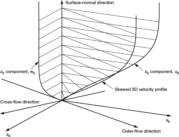
Figure 4.2.2 Isometric view of the 3D boundary-layer velocity profiles of Figure 4.1.6, as resolved in an arbitrary 3D boundary-layer coordinate system x_b, z_b

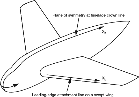
Figure 4.2.3 Examples of aligning one coordinate of a 3D coordinate system with a line along which plane-of-symmetry equations apply

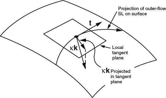
Figure 4.2.4 Illustration of outer-flow streamline curvature. The unit tangent vector to the local outer-flow streamline projection is t, and the unit curvature vector k is given by (1/κ) dt/ds. The component of the curvature vector κk projected in the local tangent plane is the component that is active in producing cross flow in a 3D boundary layer

Another way to look at the active component of the curvature is to project the outer streamline into the tangent plane instead of into the surface itself. The perpendicular component of κk, which is the one due to surface curvature, is then lost (zero), but the parallel component is the same as before. So the curvature we're interested in is the curvature of the outer streamline as viewed in the local tangent plane. For a curve that lies in a curved surface, the mathematical term for this part of the curvature is intrinsic curvature. So pressure-driven cross flow is always associated with situations in which the intrinsic curvature of the outer-flow streamlines is nonzero.

When a curve lying in a surface has zero intrinsic curvature it is called a geodesic of the surface. Longitude lines and great-circle routes on a spherical globe are examples of geodesics of a spherical surface. Sedney (1957), using the 3D boundary-layer equations in streamline coordinates, showed that if the outer-flow streamlines are geodesics of the body surface, the 3D boundary layer will have no tendency to generate cross flow. While this sounds like a very general result, the only common examples of it are axisymmetric and 2D planar flows.

Earlier in this section, we discussed how a solution to the 2D boundary-layer equations at one station along the surface depends only on what happens upstream and influences only what happens downstream, when the imposed pressure p(x) is held fixed. The same principle applies in solutions to the 3D boundary-layer equations, but we must generalize the meaning of “upstream” and “downstream” in a particular way. For the 3D boundary-layer solution along a particular column normal to the surface at a point P, when the imposed pressure p(x_b, z_b) is held fixed, the upstream zone of dependence and the downstream zone of influence are curvilinear wedge-shaped regions defined by the widest range of streamline directions passing through the column, as shown in Figure 4.2.5 (see Wang, 1971). The flow at every point on the column at P depends on everything inside the upstream zone of dependence and influences everything in the downstream zone of influence. In the lateral regions outside of both of these zones, the flow neither directly affects, nor is directly affected by, the flow at points along the column at P. As was the case in 2D, this all- or-nothing dependence/influence situation is an idealization resulting from the theoretical assumptions. The earlier comments regarding indirect influence through interaction with the outer flow and the effects of local disturbances like small bumps on the surface apply in 3D as they did in 2D. In 3D we have the additional effect of viscous diffusion in the lateral cross-stream direction, which is ignored in the idealized theory but which can have direct effects in the real world that are significant over short distances, on the order of the boundary-layer thickness. Thus it would be reasonable to think of direct dependence and influence in the real world as a kind of blurred version of the picture in Figure 4.2.5.

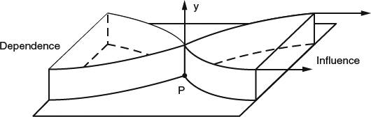
Figure 4.2.5 Zones of dependence and influence in the 3D boundary-layer equations

4.2.2 Integrated Momentum Balance in a Boundary Layer

Looking at the streamwise momentum balance in the boundary layer in an integrated sense is informative for purposes of physical understanding and is the basis for a whole class of boundary-layer prediction methods, the integral methods. If we take the 2D momentum Equation 4.2.1, substitute Equation 4.2.5 for the dp/dx term, and integrate in the y direction from y = 0 to any height h that is everywhere outside the boundary layer, we obtain

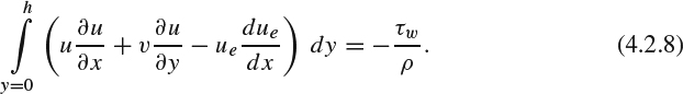
Then if we integrate the continuity Equation 4.2.4 from y′ = 0 to y′ = y and substitute for v in Equation 4.2.8, recognizing that

we obtain the von Karman momentum integral equation:

where

is the boundary-layer momentum thickness, and

is called the boundary-layer shape factor, and δ* is the displacement thickness, a measure of the displacement effect of the boundary layer, which we'll discuss below (Equation 4.2.13). The second term on the right-hand side defines the effect of the pressure gradient and is shown in two alternate forms, one using du_e/dx and the other using dp/dx directly. The two forms are related by the Euler momentum Equation 4.2.5. A version of Equation 4.2.10 valid for compressible flow can be found in Schlichting (1979).

The momentum thickness is a measure of the flux of momentum deficit and can be related to drag in ways we'll discuss in Section 6.1.4. The flux of momentum deficit isn't the easiest of concepts to appreciate intuitively, but it leads to the most direct way to express the integrated momentum balance, as in Equation 4.2.10.

As we'll see in Section 4.4, Equation 4.2.9 holds for turbulent flow as well as laminar, so that the momentum integral Equation 4.2.10 is valid for turbulent flow, even though we derived it from the field equations for laminar flow.

The momentum integral equation quantifies and illuminates several important relationships in boundary-layer flows. It clearly shows how the growth of the boundary layer, represented by dθ/dx in Equation 4.2.10, depends on the skin friction and the pressure gradient, relationships we discussed in physical terms in Section 4.1.2. It dictates that the growth rate dθ/dx will be positive unless the pressure-gradient term is sufficiently negative (i.e., there is a sufficiently strong favorable pressure gradient) to offset the skin-friction contribution. It also shows how the effect of the pressure gradient depends on the shape of the velocity profile, through the shape factor, H. Referring to the laminar velocity profiles with low and high H sketched in Figure 4.2.6, we can see that the higher H is, the higher will be the proportion of the flux of momentum deficit that is accounted for by low-velocity fluid. As we argued in Section 4.1.2, low-velocity fluid responds to the pressure gradient with a larger local velocity gradient ∂u/∂x. A high-H boundary layer is thus more susceptible to the effect of a pressure gradient, an effect that Equation 4.2.10 quantifies in terms of dθ/dx.

The momentum integral equation has four independent variables: u_e, θ, H, and C_f. Generally at least one of these must be imposed as a “boundary condition.” Solving the equation with u_e imposed is referred to as the direct mode, just as it was in solving the field Equations 4.2.1–4.2.4. And just as before, solving with any of the other three imposed instead is referred to as an inverse mode. Whatever mode the equation is solved in, it has three unknowns, and two additional closure relationships are therefore required in order to have a complete system. One relation is almost always a skin-friction law that defines C_f as a function of other boundary-layer quantities. In many methods, the other closure relation requires making an assumption about the velocity profiles, usually in the form of a family of profile shapes with a range of shape factor H. The skin-friction law and the other closure relation will of course depend on whether the flow is laminar or turbulent. A wide variety of integral boundary-layer methods have been developed for both laminar and turbulent flow. Two of the best-known examples are the lag-entrainment method of Green, Weeks, and Brooman (1977) for turbulent flow, and the laminar and turbulent methods developed by Drela and Giles (1986) for airfoil calculations. White (1991) discusses some of the earlier methods.

Three-dimensional integral boundary-layer equations can be derived in the same way, starting with the 3D boundary-layer momentum equations in general curvilinear, nonorthogonal coordinates. There are then two equations corresponding to Equation 4.2.10, one for each in-surface coordinate direction. Because there are two surface-parallel velocity components carrying momentum, the equations contain two “displacement” thicknesses and four momentum thicknesses. There are also two skin-friction coefficients to solve for. Compared with 2D, we thus have five more basic unknowns and only one more basic equation, so more closure relations are required. Tying the additional integral thicknesses together generally requires making empirical assumptions about the velocity profiles. The usual approach is to develop relations based on empirical models for the streamwise and cross-flow velocity profiles and then to transform the relations into the general coordinate system. The resulting equations are very complicated. The 3D integral method by P.D. Smith (1972) is one of the better-known examples.

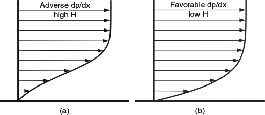
Figure 4.2.6 2D laminar velocity profiles illustrating low and high shape factor H

4.2.3 The Displacement Effect and Matching with the Outer Flow

In early applications of boundary-layer theory, p(x) or u_e (x) was usually assumed to be known a priori from a potential-flow solution for inviscid flow around the body, the boundary-layer equations were solved in the direct mode, and any influence of the boundary layer on the outer flow was ignored. Later development of the rigorous theory showed that this is all that is required for the formal first-order theory. But in many practical applications, the effect of the boundary layer on the pressure distribution is significant, and the first-order theory is not enough.

In higher fidelity viscous-inviscid matching calculations, the objective is to impose the boundary layer's displacement effect on the outer flow and thus to have the outer-flow calculation provide a prediction of the boundary-layer's effect on the surface pressure. Note that the correction for displacement is formally a second-order effect (see White, 1991, Section 4.11), but that when we introduce it we still usually ignore all other second-order effects. Interactive schemes that impose the displacement effect always require some iteration, with both the boundary-layer and the outer-flow solutions repeated several times.

The most obvious matching strategy is simple repeated cycling: Calculate the inviscid flow, then input the resulting u_e (x) to a boundary-layer calculation, and then add the resulting δ* to the body shape, and repeat to the inviscid calculation. This scheme works some of the time, but it doesn't always converge, especially if the boundary-layer calculation gets close to separation. Many other schemes have been developed in attempts to achieve more robust convergence, to extend matching calculations into regions of separation, and to reduce computing time. In these schemes, the inviscid flow and the boundary layer are calculated either in series or in parallel with each other, or simultaneously in systems where the boundary-layer and outer-flow equations have been combined. In various nonsimultaneous schemes, the boundary-layer equations may be solved in the direct mode, an inverse mode, or a combination. In all cases, the matching of p(x) or u_e(x) is either imposed explicitly as a condition on each boundary-layer solution or is sought as an outcome of the iterative coupling. We'll discuss such schemes further in Chapter 10.

In Section 4.1.3, we discussed the displacement effect and the idea of a displacement thickness in qualitative terms. We also discussed the concept of an equivalent inviscid flow, which has the same velocity field and pressure distribution outside the boundary layer as the actual flow, but remains inviscid and irrotational across all or part of the near-wall region occupied by the boundary layer in the actual flow. Implementing this concept requires altering the boundary conditions on the outer inviscid flow solution so that it matches the desired equivalent inviscid flow. There are two ways to do this: (i) to apply the usual no-through-flow boundary condition on an “effective” body contour that has been moved outward by the displacement thickness or (ii) to apply a nonzero normal velocity, or transpiration, on the actual body contour. These ideas are illustrated in Figure 4.2.7.

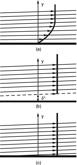
Figure 4.2.7 Illustration of the 2D boundary-layer displacement effect. (a) Actual boundary-layer flow. (b) Equivalent inviscid flow with displacement thickness. (c) Equivalent inviscid flow with surface transpiration

In Section 4.1.3, we saw that in 2D flows the most convenient value for the displacement thickness δ* can be defined by requiring that the equivalent inviscid flow between y = δ* and any value of y outside the boundary layer, as shown in Figure 4.2.7b, have the same mass flow as the actual flow, as shown in Figure 4.2.7a. The result is that δ* is given by an integral of the local velocity profile:

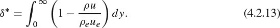
Given this definition, the imaginary displacement surface at y = δ* is a streamline of the equivalent inviscid flow and is therefore a surface along which the equivalent inviscid flow would satisfy a solid-wall boundary condition.

But this is not our only choice for a definition of δ*. As we noted in Section 4.1.3, we can apply a solid-wall boundary condition at any nearby streamline of the equivalent inviscid flow, and it will have the same effect on the rest of the flow. Thus the value of δ* defined by Equation 4.2.13 isn't the only choice that would have the effect we seek. However, as we saw in Figure 4.3.12, the drawback to the other choices for δ* is that the displacement surface won't have a simple, closed shape at the nose of the body. As a practical matter, this is a major drawback, and alternative definitions of 2D δ* are never used in practice. But the alternative derivation is useful because it shows the way toward a definition of δ* that works in 3D.

The alternative derivation of 2D δ* that captures the other possible choices is based on flow tangency and the continuity equation. Recall from Section 4.1.3 that the purpose of defining δ* is to produce the right flow inclination v/u_e in the equivalent inviscid flow where it contacts the displacement surface. We can calculate v(y) in both the real flow and the equivalent inviscid flow by integration of the continuity equation in the y direction. For the real flow, we start with v = 0 at y = 0 and integrate outward to a point outside the boundary layer. For the equivalent inviscid flow, we start with v matching the real flow outside the boundary layer and integrate inward to any y inside the boundary layer, thus defining v(y) for the equivalent inviscid flow. The δ* surface we seek to define must be tangent to the streamlines of the equivalent inviscid flow and thus must have a slope dδ*/dx equal to v(y)/u_e. The result is an equation for δ*:

where is defined by the local integral given by Equation 4.2.13. Equation 4.2.14 is singular at a stagnation point, but useable elsewhere. When Equation 4.2.14 is integrated in x, it defines δ* only to within a constant of integration. In effect, the value of δ* at any initial x station other than the stagnation point is free to be chosen arbitrarily.

At the stagnation point of attachment, we seem to have a problem: Equation 4.2.14 is singular there, and because u(y) = u_e = 0, Equation 4.2.13 doesn't seem to define anything either. But the 2D stagnation-point boundary layer is one of the laminar similarity solutions we'll discuss in Section 4.3.2, and in the neighborhood of the stagnation point is constant, including in the limit as the origin is approached. So is the definition of δ* that works at the stagnation point and is consistent with Equation 4.2.14 elsewhere.

In 3D flow, the mass-flux argument leading to Equation 4.2.13 doesn't generally apply. Instead, we must use the same matching and tangency analysis that led to Equation 4.2.14, extended to 3D flows (see Nash and Patel, 1972). The result is a PDE in two dimensions on the body surface, involving two local integrals of the velocity profiles, which in Cartesian coordinates is given by

where q_e is the edge-velocity magnitude , and

The 3D δ* equation is hyperbolic, and solving it numerically must follow the usual rules for hyperbolic equations. Initial conditions (initial values of δ*) must be defined at upstream boundaries, in a manner analogous to defining a starting value of δ* in 2D in Equation 4.2.14. Three-dimensional analogs to starting at a 2D stagnation point are starting at a singular point of attachment, as at the blunt nose of a fuselage, or at an attachment line, as at the leading edge of a swept wing. A similarity solution applies at a singular point of attachment, and at a leading edge attachment line, we can usually use the plane-of-symmetry boundary layer equations discussed in Section 4.3.4. Both of these situations define starting values of δ* analogous to starting with in 2D.

We mentioned earlier that an alternative to using δ* to produce the displacement effect is to use an equivalent transpiration boundary condition applied at the actual body surface. We derive this condition by applying the same process of integrating the continuity equation that led to Equations 4.2.14 and 4.2.15. The 2D result is

and the 3D result for Cartesian coordinates is

or, given Equation 4.2.15,

Imposing this as a boundary condition on the outer flow simulates the boundary-layer displacement effect by enforcing the flow situation illustrated in Figure 4.2.7c. Note that because this is a boundary condition on the outer inviscid flow, ρ_w is the density of the inviscid flow at the wall, not the viscous boundary-layer flow.

4.2.4 The Vorticity “Budget” in a 2D Incompressible Boundary Layer

In Section 3.6, we discussed the vorticity equation governing the creation or destruction, convection, stretching, and diffusion of vorticity. In a 2D planar flow, only the transverse component of the vorticity can be nonzero, and there is no vortex stretching. Furthermore, if the density is constant, there can be no creation or destruction of vorticity in the interior of the field. With these restrictions, there is only convection and diffusion, and the vorticity equation looks like a conservation equation for a passive scalar (the transverse component of the vorticity). We should keep in mind, however, that it isn't an independent physical equation in its own right, but really just a sort of rearrangement of the momentum equation.

In a 2D, incompressible, steady flow, the conservation of vorticity in control-volume form is quite simple. It reduces to a balance between two fluxes integrated over the boundaries of the control volume: the convective flux and the diffusive flux v∂ω/∂n, where v is the kinematic viscosity, and ω is the vorticity component in the transverse direction, the only component that can be nonzero.

In Figure 4.2.8, we set up a control volume for a boundary-layer flow in the x direction and indicate the relevant diffusive flux to or from the wall and the convective fluxes through the upstream and downstream boundaries. The diffusive fluxes at the upstream and downstream boundaries are negligible. Even if flow passes through the outer boundary, there is no diffusive or convective vorticity flux there because the vorticity is effectively zero outside the boundary layer. So the diffusive flux in or out at the wall must balance the difference between the convective flux in (upstream) and out (downstream).

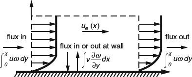
Figure 4.2.8 Control volume for tracking the vorticity “budget” of a 2D incompressible boundary layer

The diffusive flux of vorticity to the wall is given by

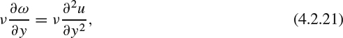
and for a thin boundary-layer flow, the convective flux reduces to

So we see that the net vorticity flux in a thin boundary layer is given approximately by half the square of the edge velocity. This is analogous to the result that the integrated vorticity in a thin shear layer is approximately equal to the velocity jump across the shear layer, which we discussed in Section 3.3.8.

Now we see that the vorticity balance requires flux to or from the wall only when u_e is changing with x. The wall acts as a source or sink for vorticity depending on the rate of change of u_e. Increasing u_e requires vorticity flux from the wall, or negative ∂²u/∂y², while decreasing u_e requires vorticity flux to the wall, or positive ∂²u/∂y². This is of course consistent with our finding in Equation 4.2.7, based on the momentum equation, that ∂²u/∂y² at the wall is proportional to dp/dx.

A flat-plate boundary layer, for which u_e is constant in x, is an interesting special case. When u_e is constant, there is no diffusive vorticity flux to or from the wall, only a constant integrated convective flux along the flow direction. Of course, the vorticity in the field becomes more diffuse as the boundary layer thickens.

4.2.5 Situations That Violate the Assumptions of Boundary-Layer Theory

Remember that in deriving Prandtl's boundary-layer equations, it was assumed that the boundary layer is thin and that x derivatives are much smaller than y derivatives. Any boundary-layer situation in which the x derivatives become comparable to the y derivatives obviously violates these assumptions. Figure 4.2.9 illustrates a few common examples of flows that constitute boundary layers in the physical sense but violate the assumptions of first-order boundary-layer theory.

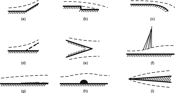
Figure 4.2.9 Illustrations of situations that violate the assumptions of first-order boundary-layer theory. (a) Corners. (b) Steps. (c) Large longitudinal curvature. (d) Separation from a smooth wall. (e) Separation from trailing edge. (f) Interaction with shock. (g) Sudden change in surface roughness. (h) Protuberances. (i) Sharp leading edge

Situations such as these can raise interesting issues for boundary-layer theory. For example, separation from a smooth wall (Figure 4.2.9d) is something we discussed from a physical point of view in Section 4.1.4, where we saw that the skin-friction coefficient C_f goes through zero at a separation point in 2D flow. Because the negative values reached by C_f downstream of separation are generally quite small in magnitude, in the real world governed by the full NS equations C_f usually goes through zero with a small slope (Figure 4.2.10a). Direct-mode solutions to the first-order boundary-layer equations don't predict this behavior correctly at all. The C_f calculated in the direct-mode goes through zero at separation with infinite slope (Figure 4.2.10b), a square-root singularity that in the context of boundary-layer theory is called the Goldstein singularity. Numerical methods for solving the equations in the direct mode generally fail before reaching the singularity. Solving the equations in any of the inverse modes removes the singularity but does not alleviate the problem that x derivatives in the neighborhood of separation are usually still large enough to violate the boundary-layer-theory assumptions.

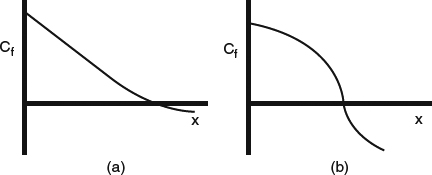
Figure 4.2.10 Illustrations of how C_f goes through zero at separation in 2D. (a) Small slope according to NS equations. (b) Infinite slope (Goldstein singularity) according to direct-mode BL equations

Continuing the solution downstream of the separation point raises another set of difficulties having to do with dependence and influence. Upstream of separation, a one-direction marching sequence can be used in the numerical scheme, because the solution at any point depends only on the solution upstream. Downstream of separation, the reversed flow at the bottom of the boundary layer convects information from the general downstream direction, and for the numerical scheme to deal with this properly, something more complicated than one-direction marching is required.

Separation from a sharp trailing edge (Figure 4.2.9e) raises a different set of issues. For this situation, an approximate correction to boundary-layer theory has been developed, called triple-deck theory (see White, 1991, for a summary). Of course, the full NS equations handle all of these situations “exactly,” and without any of the previous theoretical difficulties, just a large increase in required computational effort.

Separation from a smooth wall in 3D raises the same issues for direct-mode solutions to the boundary-layer equations as it does in 2D. The component of C_f perpendicular to the separation line goes through zero with a square-root (Goldstein) singularity just as 2D C_f does. This means that adjacent skin-friction lines converge to a distinct separation line parabolically, rather than just asymptotically converging toward each other, as they do in solutions to the NS equations. This distinction is illustrated in Figure 4.2.11. Some illustrations of the topology of separation, such as the one in Figure 4.1.17, show the separation line in the form of a distinct, singular line, as in Figure 4.2.11b, even though separation in real flows takes the form in Figure 4.2.11a.

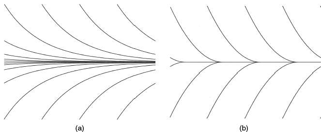
Figure 4.2.11 Skin-friction lines in neighborhood of a 3D separation line. These are the 3D analogs of the 2D C_f distributions of Figure 4.2.10. In 3D, the component of C_f perpendicular to the separation line follows qualitatively the same pattern as in 2D. (a) Continuous variation according to NS equations (asymptotic convergence). (b) Singular behavior according to direct mode BL equations (parabolic convergence)

4.2.6 Summary of Lessons from Boundary-Layer Theory

To summarize the conclusions we've gleaned from boundary-layer theory:

1. Because a boundary layer tends to remain thin, the pressure variation across it tends to be small and is ignored in the first-order theory. The pressure plays the role of an environmental condition imposed on the boundary layer from outside, that is, by the outer inviscid flow.
2. The local flow in the boundary layer depends on everything that happens upstream and influences everything that happens downstream.
3. The local boundary layer's influence on what happens upstream is much less direct. If the boundary layer is attached, it has little direct influence upstream (none in the first-order theory), and only a weak indirect influence through the outer flow. If the boundary layer separates, its upstream influence through the outer flow becomes much stronger.
4. The development of a 2D laminar, incompressible boundary layer, expressed in dimensionless terms, is independent of Reynolds number, provided the boundary layer starts at a stagnation point.

Except for point (4), the above conclusions apply to both 2D and 3D boundary layers.

4.3 Flat-Plate Boundary Layers and Other Simplified Cases

In this section, we look at flat-plate flows and a number of other situations in which boundary-layer behavior is simplified in one way or another. These idealized cases provide valuable physical insights that are not as easily seen in more general situations. And in many situations, they are close enough to reality to provided useful quantitative information.

4.3.1 Flat-Plate Flow

When the outer-flow pressure and velocity are constant in 2D flow, the flow development predicted by boundary-layer theory is particularly simple. This idealized situation is referred to as flat-plate flow because a thin flat plate aligned with the flow actually produces something very close to it, except in the neighborhood of the leading edge.

Two-dimensional incompressible laminar flow at constant pressure is one of the similarity situations we mentioned in Section 4.2.1, and the similarity solution is credited to Blasius (see Schlichting, 1979). Treating the corresponding incompressible turbulent flow requires empiricism to account for the effects of turbulence, which we'll consider in more detail in Section 4.4.2.

Expressions for the average skin-friction coefficient over the length of a flat plate are widely used in preliminary drag estimation, as we'll see in Section 6.2.1. A question mark that hangs over any such formula has to do with the leading-edge region and what details had to be glossed over there. If we start the boundary layer at zero thickness and ignore the singularity of the boundary-layer equations in that situation, not to mention the fact that the assumptions behind the equations aren't valid there, the result from the Blasius solution for incompressible laminar flow is

The most widely used corresponding formula for incompressible turbulent flow is the Prandtl-Schlichting relation (see Schlichting, 1979):

These laminar and turbulent relations are plotted for a wide range of length Reynolds number in Figure 4.3.1. First, note that in both laminar and turbulent flow decreases with increasing Reynolds number, in spite of the fact that the boundary-layer thickness, as a fraction of body length decreases and ∂u/∂y at the wall (in dimensionless terms) increases. The rate of increase of dimensionless ∂u/∂y at the wall is not enough to cancel the direct effect of the Reynolds-number increase. Also note that laminar decreases faster than turbulent , becoming a smaller and smaller fraction of turbulent .

The curves for cases with transition in Figure 4.3.1 were calculated for idealized “instantaneous” transition, in which the boundary layer is assumed to become turbulent immediately at the assumed transition location, and the turbulent boundary layer is assumed to start with the same momentum thickness reached by the laminar boundary layer at the transition point. (We'll see immediately below how θ and are related, in Equation 4.3.3.) Note that when the length Reynolds number exceeds the assumed transition Reynolds number, and the boundary layer becomes turbulent on the downstream part of the plate, the average C_f increases rapidly at first and then asymptotically approaches the all-turbulent curve from below.

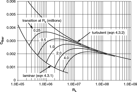
Figure 4.3.1 Average skin-friction coefficients for incompressible laminar, transitional, and turbulent flow on a flat plate

Because the pressure gradient is zero in flat-plate flow, only the skin friction contributes to the growth in momentum thickness along the plate. θ is then just proportional to the cumulative average , as can be seen in the momentum-integral Equation 4.2.10, which reduces to

This result is valid for either laminar or turbulent flow and is not limited to incompressible flow.

The local C_f is often also of interest, and we can obtain expressions for it by differentiating , where comes from Equations 4.3.1 and 4.3.2. The result for incompressible laminar flow is

and for incompressible turbulent flow:

These relations are plotted in Figure 4.3.2. The first thing to note about local C_fi is that it decreases with increasing R and is therefore less than (for flat-plate flow; in more general situations, this is not always the case). The cases with transition are the same ones for which was plotted in Figure 4.3.1, but when viewed in terms of C_fi in Figure 4.3.2, they look very different. After transition, local turbulent C_fi jumps well above the all-turbulent curve. This is because the laminar run results in a thinner boundary layer (smaller θ) at the start of the turbulent boundary layer than would be there in the all-turbulent case. Thus the local-C_fi curves in Figure 4.3.2 approach the all-turbulent curve from above, while the curves of Figure 4.3.1 approach it from below because the average includes the low-C_f laminar run.

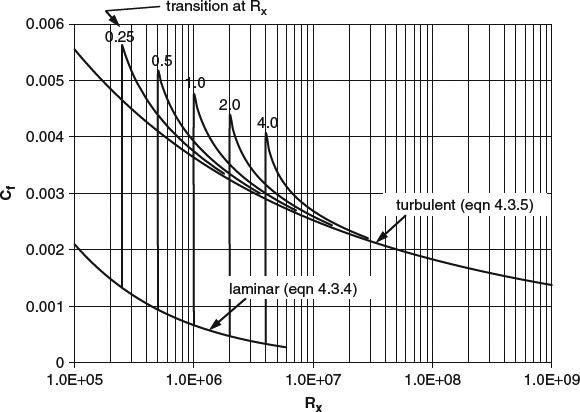
Figure 4.3.2 Local skin-friction coefficients for incompressible laminar, transitional, and turbulent flow on a flat plate

The above formulas for and C_fi as functions of x are not always accurate for real-world flat-plate flows because the development of a real flow near the leading edge doesn't generally follow the idealized flat-plate assumptions. Away from the leading edge, real-world flows with constant pressure should settle into agreement with the local-C_f formula, but with a shift in the apparent origin in x. In the “fully developed” flat-plate boundary layer the local relationship between C_fi and R_θ is independent of what happened near the leading edge. For laminar flow, we can derive this formula by inverting Equation 4.3.4 (expressing x as a function of C_fi) and substituting it into Equation 4.3.3, with the result:

For turbulent flow, Equation 4.3.5 cannot be inverted in closed form, and the turbulent counterpart to Equation 4.3.6 must be determined by numerical interpolation of tables of C_fi(x) from Equation 4.3.5 and R_θ (x) from Equations 4.3.2 and 4.3.3. The resulting C_fi(R_θ) relations are plotted in Figure 4.3.3.

Compressibility and/or heat transfer can alter flat-plate skin friction significantly. For cases with heat transfer, numerical calculations are generally required. For the case of an adiabatic wall, the situation is simpler, and many approximate theories have been developed, with predictions that vary widely (see White, 1991). Experimental data from numerous sources also show considerable scatter. White states that the curve labeled “Frankl-Voishel” in his Figure 7.22 fits “typical data” fairly well. A simple formula that approximately fits this curve, over the range of Mach numbers below 2.0, is given by

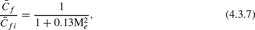
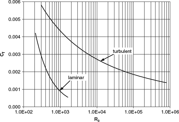
Figure 4.3.3 Local skin-friction coefficients for incompressible laminar and turbulent flow on a flat plate, as functions of R_θ

which is plotted in Figure 4.3.4. Note that at Mach 1.0, compressibility reduces by only about 10%.

4.3.2 2D Boundary-Layer Flows with Similarity

Similarity in a boundary-layer flow refers to a situation in which the velocity profile in nondimensional form, with an appropriately scaled vertical coordinate, is the same for all x. Strictly speaking, similarity exists only in laminar flow, but there are examples of near-similarity in turbulent flow.

For incompressible laminar flow, it can be shown that similar solutions exist when u_e ∼ x^m. In such cases, a similarity transformation can be defined that reduces the boundary-layer Equations 4.2.1 and 4.2.4 to a single ODE. A derivation is given in Schlichting (1979). The ODE has solutions for a range of values of m, which are usually referred to in terms of the value of the similarity parameter β = 2m/(m + 1). Negative values of β correspond to adverse pressure gradients, with a boundary layer in a constant state of incipient separation (zero C_f for all x) corresponding to β = −0.19884. Zero β corresponds to a flat-plate flow (constant u_e, the Blasius solution), and positive β corresponds to favorable pressure gradients. Velocity profiles for three representative values of β are plotted in Figure 4.3.5.

The laminar similarity solutions are often referred to as wedge flows because the outer-flow velocity distribution u_e ∼ x^m arises in the potential flow around a wedge of included angle πβ. These are the same corner-flow solutions that we saw in Section 3.10 can be obtained by conformal mapping. Figure 4.3.6 illustrates how they work for the different types of flow. The decelerating flows correspond to wedges with negative included angles, or potential flow over a convex corner, as in Figure 4.3.6a. Flat-plate flow corresponds to a zero included angle, as in Figure 4.3.6b, and β = 1 corresponds to a 2D stagnation-point flow, as in Figure 4.3.6c, often referred to as Hiemenz flow. Note in Figure 3.10.2 that the edge velocity in the stagnation-point flow increases linearly away from the stagnation point, and the laminar-boundary-layer thickness is constant because the usual tendency of a boundary to grow is canceled by the strong favorable pressure gradient.

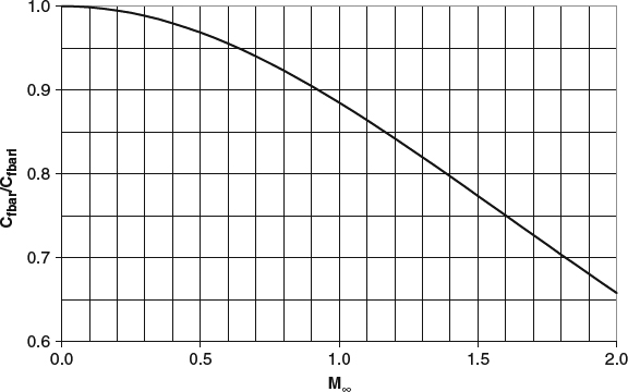
Figure 4.3.4 Effect of Mach number on adiabatic turbulent skin friction on a flat plate, Equation 4.3.7

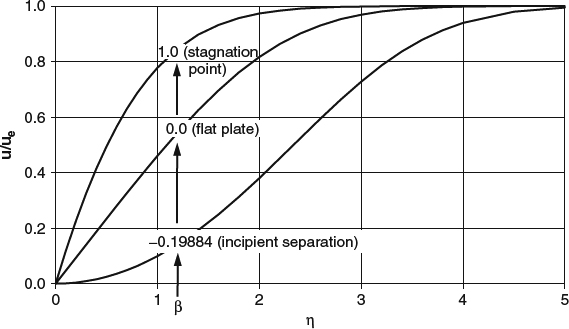
Figure 4.3.5 Velocity profiles for several laminar similarity solutions with outer-flow velocity distributions corresponding to the potential flow over wedges with included angles πβ, as illustrated in Figure 4.3.6. η is the dimensionless normal coordinate =

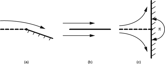
Figure 4.3.6 Illustration of the potential-flow wedge angles πβ corresponding to the laminar-boundary-layer similarity solutions. (a) Decelerating flow with negative included angle. (b) Flat-plate flow with zero included angle. (c) Accelerating flow in the special case of a 2D stagnation point flow (β = 1.0)

Of all of these similarity solutions, only two tend to appear in actual flowfields in something close to their ideal form: the flat-plate flow and the 2D stagnation-point flow. However, the other members of the laminar similarity family provide fairly good matches to local velocity profiles in more general laminar flows. As we discussed in Section 4.2.2, integral methods for predicting boundary-layer development often use assumptions about velocity-profile shapes. The laminar method developed by Drela and Giles (1986), for example, uses curve-fits based on the laminar similarity solutions.

In 2D incompressible turbulent flow, the velocity profiles themselves are never really similar, but the velocity-defect profiles, properly scaled, can be similar under the right conditions. Clauser (1954, 1956) found that if the u_e(x) distribution is properly tailored, the velocity-defect profile in the form (u_e − u)/u_τ can be held constant, where is the friction velocity, which we'll discuss further in Section 4.4.2. The defect profile is a function only of a turbulent pressure-gradient parameter,

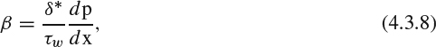
not to be confused with the laminar similarity parameter of the same name. Note that the laminar and turbulent versions of β have opposite signs: laminar accelerating flows have positive β, while turbulent accelerating flows have negative β. The turbulent similarity relation has the form

Clauser (1954, 1956) coined the term equilibrium turbulent boundary layer for the special boundary-layer flows that obey the above relation. In principle, an equilibrium turbulent boundary layer is strictly similar only in the defect-profile sense of Equation 4.3.9, but because u_τ varies slowly with x, it will appear nearly similar in terms of the conventional velocity profile, provided the range of Reynolds number considered is not too wide.

Several researchers have succeeded in setting up experimental flows that were very close to “equilibrium” in the sense of Equation 4.3.8, ranging from strongly accelerating flows (negative β) to strongly decelerating (positive β). Flat-plate flow is a member of this family. The best-known of the non-flat-plate cases was published by Stratford (1959b), a turbulent boundary layer held in a constant state of incipient separation (nominally zero C_f), which we'll see in Section 7.4.3 has played a role in the theory of airfoil maximum lift.

Like the laminar similarity solutions, the family of equilibrium turbulent-boundary-layer velocity profiles has provided velocity-profile assumptions for integral methods of calculating boundary-layer development. The turbulent method by Drela and Giles (1986) is one example.

4.3.3 Axisymmetric Flow

Axisymmetric flow generally requires an axisymmetric body shape and zero angle of attack. Flow quantities by definition depend on only two coordinates (x, r), so that axisymmetric flow is 2D, mathematically speaking. What makes axisymmetric flow different from the usual planar 2D flow is that the body radius can vary with x, contracting or stretching the boundary layer circumferentially, as illustrated in Figure 4.3.7. The flux of momentum deficit in the boundary layer is thus distributed over a varying distance circumferentially, so that the radius variation joins with the skin friction and the pressure gradient as an additional factor that affects the evolution of the boundary-layer thickness along the body. When the radius grows, stretching the boundary layer circumferentially, the rate of boundary-layer growth is reduced or even reversed, and when the radius shrinks, the rate of boundary-layer growth is increased, compared with what it would be in a planar flow with the same pressure gradient.

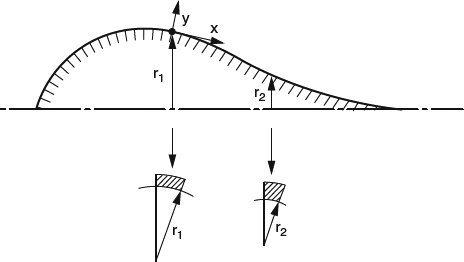
Figure 4.3.7 Illustration of the effect of a change in body radius on a boundary layer in axisymmetric flow

These effects of radius variation are similar to the effects of convergence and divergence in 3D boundary layers that we discussed in Section 4.1.2, with the major difference that in more general 3D flows the effects are often enhanced by pressure-driven cross flow in the boundary layer. In axisymmetric flow, symmetry does not allow a pressure gradient in the cross-flow (circumferential) direction, so there is nothing to drive pressure-driven cross flow. Thus unless the body is spinning, producing shear-driven cross flow, there is no cross-flow in axisymmetric flow. In mathematical terms, the outer-flow streamlines are along longitude lines of the body surface. They are therefore geodesics of the body surface, defined by having zero intrinsic curvature, so that there is no tendency to produce pressure-driven cross flow, as we discussed in Section 4.2.1.

An axisymmetric body can either be simply connected, with no “holes,” or it can be in the form of a ring with an open duct along the axis, as illustrated in Figure 4.3.8. If the leading “lip” of a ring-type body is blunt, the attachment of the flow to the lip will look locally like flow attachment to the leading edge of a 2D airfoil, and the boundary layer at the attachment will closely resemble the 2D similarity solution for β = 1 (Hiemenz flow, Section 4.3.2). If the nose of a simply connected body is blunt, flow attachment will be at a singular point of attachment, from which the flow spreads out radially, as in Figure 4.3.9. In the axisymmetric case, the boundary-layer equations for this flow can be transformed to the same ODE as for the similarity solution for 2D planar flow with β = 1/2, and the velocity profiles are therefore the same (see Schlichting, 1979). The boundary-layer thickness δ is constant in the neighborhood of the stagnation point, as it is in 2D planar flow.

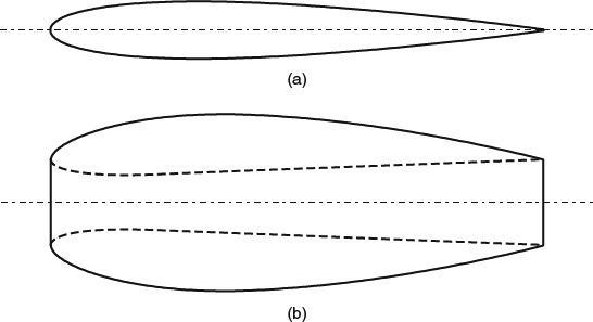
Figure 4.3.8 Illustration of two types of axisymmetric body. (a) Simply connected. (b) With open duct along axis

Figure 4.3.9 The boundary layer at a singular axisymmetric stagnation point of attachment

4.3.4 Plane-of-Symmetry and Attachment-Line Boundary Layers

Flows that have a nominal plane of symmetry are common in applications, as, for example, in the flow along the keel line of a ship hull at zero yaw or the flow along the vertical symmetry plane (crown and keel lines) of a fuselage at zero yaw. Another class of examples comes from the world of boundary-layer experiments. Many boundary-layer measurements have been made in special-purpose flow channels (air or water tunnels). The measurements are usually made in the boundary layer along the centerline of the channel floor or ceiling, and the channel sidewalls are usually parallel, with the intention of producing a 2D flow on the “test wall.” But such setups usually produce significant unintended three dimensionality because of boundary-layer growth on the sidewalls and 3D flow effects in the corners.

Plane-of-symmetry flows generally differ from 2D planar flows in that the flow off of the plane of symmetry is either diverging away from the plane or converging toward it. In an axisymmetric flow, the flow along every longitude line of the body is a special case of plane-of-symmetry flow, with convergence or divergence if the body radius is changing with x. Why is axisymmetric flow a special case? Recall from Section 4.3.3 that an axisymmetric flow produces no pressure-driven cross flow. General plane-of-symmetry flows don't have this restriction: Off of the plane of symmetry, there can be pressure-driven cross flow. Whether the convergence or divergence involves cross flow or not, it can have a significant effect on the development of the boundary-layer velocity field, as we discussed in Section 4.3.3 in connection with axisymmetric flow.

The general situation in an idealized plane-of-symmetry flow is sketched in Figure 4.3.10. On the symmetry plane, the velocity profile is parallel to the plane and looks like a 2D boundary-layer profile. Off of the symmetry plane, divergence is shown, accompanied by pressure-driven cross-flow in which the divergence velocity component peaks inside the boundary layer with a larger value than at the edge.

The 3D boundary-layer equations are of course applicable to such flows, but we can take advantage of the symmetry to reduce the equations to a spatially 2D set that applies just on the symmetry plane itself. Starting with the 3D equations, the z-momentum equation degenerates to 0 = 0 on the symmetry plane because the w velocity component is zero, and ∂/∂z of all flow quantities other than w is zero. But differentiating the equation in the z direction turns it into a nondegenerate equation for the convergence/divergence profile ∂w/∂z. For laminar constant-property flow in Cartesian coordinates, the resulting equations are:

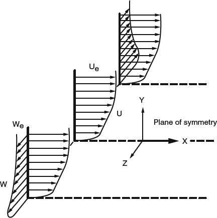
Figure 4.3.10 Sketch of a boundary-layer flow with convergence or divergence about a plane of symmetry

• x momentum:

  

• z-differentiated momentum:

  

• Continuity:

  

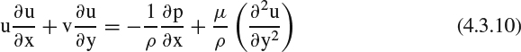
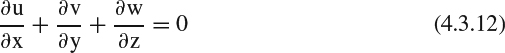
Note that the x-momentum equation is the same as the 2D boundary-layer momentum Equation 4.2.1 with no explicit appearance of ∂w/∂z. The solution for the u velocity profile is thus affected by ∂w/∂z only through the continuity equation and its effect on the vertical velocity v.

Although the plane-of-symmetry x-momentum equation is the same as in 2D flow, the momentum-integral equation picks up an additional term representing the effects of convergence/divergence. Recall that the derivation of the 2D momentum-integral Equation 4.2.10 made use of the continuity equation. In plane-of-symmetry flow, ∂w/∂z appears in the continuity equation and thus shows up in the integrated momentum equation

as the integral of ∂w/∂z weighted by the velocity defect u_e − u. This is consistent with the intuitive idea that the streamwise momentum balance is affected when momentum-deficient air is carried away by flow divergence. However, this intuitive interpretation applies directly only in the integrated sense of Equation 4.3.13. In the differential form of the momentum Equation 4.3.10, convergence or divergence is “felt” only “indirectly” through the v∂u/∂y term.

Throughout the development of CFD codes for turbulent flows, the unintended three dimensionality (convergence/divergence) of nominally 2D boundary-layer experiments has been a problem for developers of turbulence models. Discrepancies between calculated and measured boundary-layer quantities are not always the fault solely of the turbulence model, but are also contributed to by convergence/divergence in the experimental flow. It takes only small amounts of convergence/divergence, usually undetectable by flow-direction measurements, to have a significant effect on the momentum thickness θ (x), for example. Mellor (1967) argued that fairer comparisons between his turbulence model and “2D” boundary-layer measurements could be made if he assumed that any discrepancy between calculated and measured θ (x) was due to convergence/divergence, and he “corrected” his calculations for it. To make the “correction,” he solved the plane-of-symmetry equations instead of the 2D equations and set the code up to solve for the unknown ∂w_e/∂z boundary condition so as to match the measured θ(x). The turbulence model was then evaluated on how well it predicted C_f(x), H(x), and detailed velocity profiles. One uncertainty in applying this calculation strategy is what to assume about the ∂w/∂z(y) profile at the initial x station, which can affect the solution over surprisingly long distances downstream.

One of the most important applications of plane-of-symmetry boundary-layer equations is to the band of flow attachment along the leading edge of a swept wing, usually called the attachment line. (In Section 5.2.2, we'll discuss how on a wing of finite span a single attachment line cannot be uniquely defined, but can for all practical purposes be pinned down very closely.) On most swept wings, the intrinsic curvature of the attachment line is small enough, and the boundary layer is thin enough, that cross flow on the attachment line itself is negligible, and the plane-of-symmetry equations apply. (See Section 4.2.1 for a definition of intrinsic curvature and a discussion of its relationship to cross flow.) In swept-wing attachment-line flow, the flow divergence is typically so strong that it keeps the boundary layer orders of magnitude thinner than it would become on a flat plate with the same streamwise distribution of edge velocity. We'll look further at the attachment-line boundary layer in our discussion of swept wings in Section 8.6.2.

4.3.5 Simplifying the Effects of Sweep and Taper in 3D

Boundary layers on swept wings, which we'll discuss in some detail in Section 8.6.2, are generally highly 3D in the sense of having strong pressure-driven cross-flow. In the most general cases, an adequate simulation of the flow requires solving the 3D boundary-layer equations. However, on well-designed swept wings, the isobars tend to line up along the constant-percent-chord lines, and simplified equations can then provide reasonably accurate predictions of boundary-layer development.

The simplest boundary-layer equations that include the effects of sweep are the infinite-span-swept-wing equations. We assume a boundary-layer coordinate system in which the two in-surface coordinates x_sp and x_ch are aligned parallel and perpendicular to the general sweep of the wing, as illustrated in Figure 4.3.11. We assume that all flow quantities are unchanging in the spanwise (x_sp) direction, as would be the case if the wing had a uniform section and infinite span. When this assumption is applied to the outer inviscid flow instead of the boundary layer, we have simple sweep theory, which we'll discuss in Section 8.6.1.

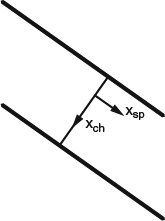
Figure 4.3.11 Coordinate system assumed in the infinite-span swept-wing boundary-layer equations

Starting with the 3D boundary-layer equations in Cartesian coordinates and setting all ∂/∂x_sp terms to zero, we obtain a set of equations that still has three velocity components, but only two space coordinates. These are the infinite-span-swept-wing boundary-layer equations, sometimes referred to as the “2.5D boundary-layer equations.” Because the spanwise coordinate x_sp no longer appears in the equations, the solution domain is only two-dimensional, along a single “cut” across the planform, in the perpendicular (x_ch) direction from leading edge to trailing edge. For purposes of numerical solution, the same upstream-to-downstream marching sequence can be used as in a 2D flow. Coding is simpler, and computing time is much shorter than for a full 3D calculation.

An important property of flows governed by these equations is that the influence that the flow in the spanwise (x_sp) direction has over the velocity profile in the chordwise (x_ch) direction is either loose or nonexistent, depending on the situation. The spanwise velocity u_sp doesn't appear in the chordwise momentum equation or in the continuity equation, so that the only way the spanwise flow can affect the chordwise flow is through the density and the viscosity (and eddy viscosity in the turbulent case). Thus for the spanwise flow to have any effect on the chordwise flow, the flow must be either compressible or turbulent. Thus in the case of laminar flow with constant properties, we have the laminar independence principle: The u_ch profile can be determined independently of the u_sp profile. This doesn't work in reverse, however. The u_sp profile depends strongly on the u_ch profile.

In turbulent and compressible flows, a rough kind of independence still tends to hold, in which the influence of the u_sp profile on the u_ch profile is weak. In Section 8.6.2, we'll look at CFD calculations that illustrate the typical magnitude of the deviation from independence in turbulent swept-wing flows.

The basic “2.5D flow” idea can be extended to wings with taper, with the help of an additional assumption. On a portion of a swept tapered wing, we can construct a coordinate system consisting of the constant-percent-chord lines (“spanlines”) and either “chordwise” arcs constructed perpendicular to them, as shown in Figure 4.3.12a or conventional “rib” cuts, as in Figure 4.3.12b. Outer-flow quantities are assumed to be unchanging along the spanlines, but we can't assume boundary-layer quantities are. So we can't just set the ∂/∂x_sp terms to zero as we did in the case without taper. But we can make an assumption about them that will still give us an equation set that is spatially “2D,” with no x_sp dependence that we have to solve for.

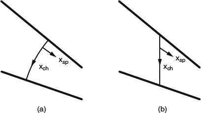
Figure 4.3.12 Coordinate systems assumed in the infinite-span swept-wing boundary-layer equations with taper. (a) A conical, orthogonal system. (b) A non-orthogonal system

We assume a kind of conical similarity in which the distribution of the outer-flow velocities (both the spanwise and chordwise components) is the same along every chordwise arc, and thus the only thing that changes for the boundary layer as we move spanwise from one arc to another is the chord Reynolds number. We also assume that the velocity profiles are similar from one arc to another, and that only the boundary-layer thickness changes, in the same way that it would change with chord and Reynolds number in a flat-plate flow. This assumption will not be satisfied exactly in turbulent flow, and we thus incur some loss of physical fidelity.

To derive the equations for tapered-wing boundary layers, we start with the 3D boundary-layer equations. For the conical coordinate system of Figure 4.3.12a, we use the curvilinear orthogonal form, and for the rib-cut system of Figure 4.3.12b, they must be in nonorthogonal form. Next we introduce a scaled normal coordinate η = y/δ. Now our assumption that the velocity profiles are similar from one arc to another is equivalent to assuming that boundary quantities are unchanging with x_sp, provided we follow them at constant η rather than constant y. For δ, we assume a flat-plate power law: for laminar flow and for turbulent flow, where c_a is the “chord” measured along the chordwise coordinate.

We'll skip the details, but when all is said and done, the infinite-span-swept-wing boundary-layer equations with taper have two types of terms that don't appear in the equations without taper:

1. Terms proportional to ∂δ/∂x_sp that arise from the ∂/∂x_sp terms in the 3D equations, which we were able to set to zero when there was no taper. Using the power law for δ(c_a), we can express these in terms of ∂c_a/x_sp.
2. Terms related to the curvature of the “chordwise” arcs (Figure 4.3.12a) or the rate of change of the skew of the coordinates (the sweep of the spanlines in Figure 4.3.12b), which is proportional to the rate of taper ∂c_a/∂x_sp.

So we've replaced the ∂/∂x_sp terms with terms containing ∂c_a/∂x_sp. There are no other x_sp-derivative terms, and we can solve the equations along a single “chordwise” cut from leading edge to trailing edge, just as we could in the case without taper. Note that if the solution is obtained along a curved arc like those shown in Figure 4.3.12a, it can be transformed to apply to any other cut across the wing (a rib cut, for example), by use of the similarity assumption and the power law for δ(c_a).

Solutions to the 2.5D boundary-layer equations are almost as simple to compute as 2D solutions, but they can predict the effects of sweep and taper on the pressure-driven cross-flow with reasonable accuracy. In Section 8.6.2, we'll compare such predictions with those made with the full 3D equations.

4.4 Transition and Turbulence

In Section 3.7, we discussed in physical terms how turbulence affects the development of a flow and how the effects can be modeled in calculations (turbulence modeling). So far in this chapter we've taken a quick look at a turbulent mean-velocity profile (Figure 4.1.4b) and we've seen how turbulent skin friction on a flat plate varies with Reynolds number (Figures 4.3.1 and 4.3.2). In this section, we'll look at how a laminar boundary layer transitions to turbulent, and then at the details of the turbulent boundary layer.

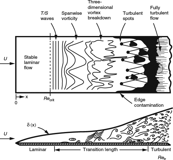
Figure 4.4.1 Possible stages in the laminar-to-turbulent transition process in a boundary layer. From White (1991). Used with permission of McGraw-Hill Companies

4.4.1 Boundary-Layer Transition

Laminar-to-turbulent transition in a boundary layer can involve a sequence of possible stages, as illustrated in Figure 4.4.1. Not all of these stages are always present, and discussions in the literature often refer to two prototypical paths to transition: (i) Natural transition, in which small disturbances grow larger through dynamic instabilities, eventually resulting in a breakdown into turbulence and (ii) Bypass transition, in which some large disturbance leads directly to turbulence, “bypassing” the process of instability growth and breakdown.

For the small-disturbance-growth phase of natural transition to be observable, the disturbance environment (freestream turbulence and acoustic levels) must be sufficiently quiet, and the surface must be smooth enough so that its interaction with the outer flow doesn't produce large disturbances. Of course, there are middle ranges of disturbance environments and surface quality in which the distinction between the two types of transition is blurred. And, of course, for transition to happen at all, conditions must be such that a turbulent boundary layer can be sustained downstream. This means that the Reynolds number must be high enough, and an extremely favorable pressure gradient cannot be present.

There is no quantitative theory for bypass transition, other than direct numerical simulation (DNS), which is almost never practical. Prediction of bypass transition is therefore practically always empirical. One application is the sizing of artificial boundary-layer tripping devices (trips), which are used in wind-tunnel testing to prevent excessive runs of laminar flow, given the low Reynolds numbers at which tests are usually run, but rarely used on actual flight vehicles. Empirical criteria for sizing trips can be found in Braslow and Knox (1958).

Predicting natural transition is important in the design of many types of flight vehicles. In Section 7.4.6, we'll look at laminar low-drag airfoils, and in Section 8.6.4, we'll consider laminar flow on swept wings. In such applications, theoretical calculations are now routinely used, but the calculations don't model the entire process, so that prediction must still rely heavily on empirical correlations.

The available theoretical framework for natural transition consists of receptivity theory, which models the process by which small environmental disturbances provide the initial amplitude for the growth of instabilities, linear stability theory, which predicts the relative rate of growth of the instabilities, once started, and nonlinear stability theory, or the theory of secondary instabilities, which extends the growth prediction into the nonlinear range. There is no quantitative theory for the final breakdown into turbulence.

Linear stability theory evolved in two major stages. In the earliest inviscid stability theories, realistic laminar-boundary-layer velocity profiles were assumed, but the flow was treated as inviscid for purposes of calculating the stability. The inviscid theory predicts that a laminar boundary layer is stable unless the velocity profile has an inflection point of the type produced by an adverse pressure gradient, as in Figure 4.1.5a. So flows with favorable pressure gradients are stable, flows with adverse pressure gradients are unstable, and flat-plate flow is neutrally stable, according to the inviscid theory. The later viscous stability theory predicts that viscosity stabilizes inviscidly unstable flows at very low Reynolds numbers, destabilizes inviscidly stable flows over a middle range of Reynolds numbers, and has a vanishing effect on stability at very high Reynolds numbers. The destabilizing effect of viscosity is crucial in the disturbance growth that leads to transition, so practical transition prediction has always relied on the viscous stability theory.

The eⁿ method was the first successful prediction method for natural transition, and elaborations on it are still the state of the art for practical prediction. In the eⁿ method, calculations are made only for the viscous linear-stability-theory phase of the disturbance growth, and transition is predicted to take place when the calculated amplitude ratio reaches a predetermined threshold value of eⁿ. In the early development of the method, the single value n = 9 was thought to be a good compromise for all flows. The resulting “e⁹ method” was reasonably successful for 2D low-speed flows, but was much less so when applied later to more-complicated flows. The current state of the art is called variable n-factor, in which a variable value of n is used to account for the initial receptivity phase, and for the final non-linear growth and breakdown (see Crouch, 2008). Receptivity theory is not used directly for any calculations, but it does provide guidance in the determination of the empirical correlations that determine n. For example, receptivity theory suggests that the effects of surface roughness should be correlated with the roughness size normalized by boundary-layer thickness, not by a roughness Reynolds number. In the variable n-factor method, receptivity plays this important secondary role, while only the linear stability theory is used directly in the calculations.

In the viscous linear stability theory, small-amplitude velocity and pressure disturbances (u′, v′, w′, p′) are assumed to be superimposed on a base steady flow with a known velocity profile. This assumption is substituted into the NS equations, terms higher than first order in the disturbances are dropped, and terms containing only the base flow are subtracted out, given that the base flow is assumed to satisfy the equations. The resulting small-disturbance equations are homogeneous and are linear in the disturbances. At the usual kinds of boundaries (a solid wall with a no-slip condition or a freestream in which disturbances are assumed to die out far away), the boundary conditions on the disturbance velocities are also homogeneous. The problem is thus an eigenvalue problem, which will be satisfied by some sequence of eigenfunctions.

There are several different ways in which the disturbance equations have been simplified and used. The disturbance pressure is generally eliminated, reducing the number of equations. One of the steps is generally to assume that the disturbance velocities can be decomposed into a series of normal modes that are oscillatory in directions parallel to the surface and in time, leaving only the dependence on y to be determined, for example:

This reduces the problem to that of finding combinations of eigenvalues (spatial wave numbers α and β, and temporal frequency ω) for which physically meaningful solutions exist, and solving for corresponding eigenfunctions v(y) that satisfy the equations. Assuming that growth takes place only in time (real α and β, complex ω) leads to the temporal stability problem, while assuming growth takes place in space (complex α and β, real ω) leads to the spatial stability problem. We can simplify the spatial stability problem further by lining the x direction up with the direction in which disturbance growth takes place, so that there is no growth in the z direction (β is real), thus reducing the number of parameters in the problem. Now ω and β (both real) are the only remaining free parameters that specify a particular disturbance mode. Once ω and β are specified, α is constrained by the eigenvalue problem, in that meaningful solutions exist only for particular values. Once α is determined, the real part defines the wavelength of the disturbance, and the imaginary part is the spatial growth rate.

Numerical solutions to the eigenvalue problem are used to determine α and thus the wavelength and the damping or growth rate of a particular disturbance. Because the theory is linear, the rate predicted is a relative rate, proportional to the current disturbance amplitude. Disturbances that are damped are referred to as stable, those that are amplified are referred to as unstable, and those on the boundary between the two are neutral. At a sufficiently low Reynolds number, all disturbances are stable. As Reynolds number increases, a critical Reynolds number is reached at which one particular disturbance crosses the neutral boundary from stable to unstable. As Reynolds number increases further, disturbances over a wider range of frequencies become unstable, and growth rates increase for the unstable disturbances.

For boundary layers, three basic types of potentially unstable modes (Figure 4.4.2) arise from the theory:

1. Tollmien-Schlichting (TS) waves, in which the velocity disturbances are “2D” in the direction perpendicular to the wave fronts. In 2D incompressible flat-plate flow, the fastest-growing modes propagate in the flow direction, while compressibility, pressure gradients, or 3D effects can bring oblique modes into play. A streamwise mode in 2D flow is illustrated in Figure 4.4.2a.
2. Cross-flow (CF) instabilities, usually in the form of stationary disturbance vortices, as illustrated in Figure 4.4.2b, which can occur in boundary layers with moderately strong cross-flow velocities. As pure disturbances, CF vortices are counter-rotating, but when the background mean vorticity of the boundary layer is superimposed on them, they appear to be co-rotating. Traveling cross-flow disturbances can be significant, but only in wind-tunnel environments with high turbulence levels.
3. Taylor-Goertler instability, counter-rotating streamwise vortices, which can occur in boundary layers on concave surfaces, as illustrated in Figure 4.4.2c.

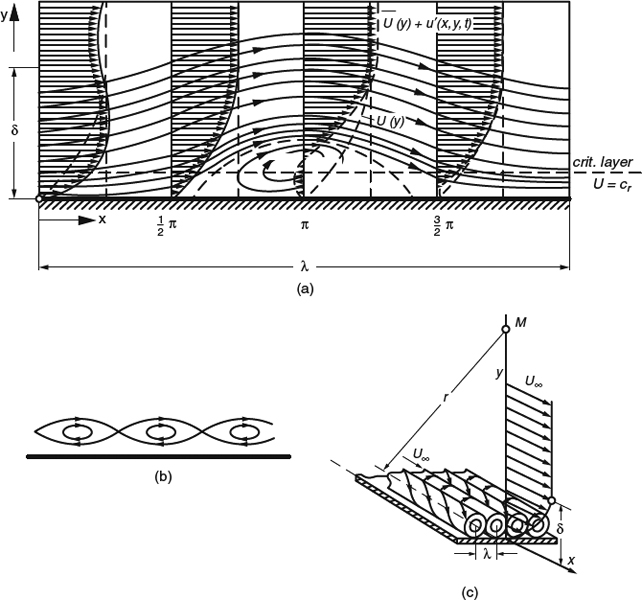
Figure 4.4.2 The three basic types of potentially unstable disturbance modes (see Reed and Saric, 1989). (a) Tollmien-Schlichting waves (2D disturbances). A case of streamwise propagation in a 2D flow is illustrated here in terms of velocity profiles and the streamline pattern. From White, (1991). Used with permission of McGraw-Hill Companies. (b) Cross-flow instability (stationary disturbance vortices, shown as a schematic streamline pattern in a plane perpendicular to the axes of the vortices). From Reed and Saric, (1989). Used with permission of Annual Review of Fluid Mechanics. (c) Taylor-Goertler instability (streamwise vortices on concave surfaces). From White, (1991). Used with permission of McGraw-Hill Companies

More than one mode may coexist in a given flow, and when their amplitudes are small, they grow independently of each other, according to the linear theory. Often, one or the other grows faster and leads to transition, as if the other mode hadn't existed. It is also conceivable that if two modes are of comparable strength when they reach the nonlinear range, that nonlinear interactions between them can play a role in transition. Figure 2.1c shows a smoke-flow visualization of the flow past a rotating body of revolution in which signs of both TS waves and vortices due to CF instability can be seen.

Real instability growth in an otherwise steady boundary layer is spatial, not temporal. But the spatial stability problem is harder to solve than the temporal problem, and in the early decades of stability research, only the temporal problem was dealt with. This turns out to have been forgivable, since the two problems lead to the same result at the neutral boundary, and early work concentrated only on determining the neutral boundaries for various boundary-layer velocity profiles. Later transition-prediction methods that depend on calculated growth rates generally use solutions to the spatial problem.

Another simplification is the assumption of parallel flow, in which the local variation of the boundary-layer velocity profiles in directions along the surface is ignored, and the base flow is assumed to depend only on y. Assuming 2D parallel flow and 2D disturbances, and eliminating u′ from the equations, results in the classic ODE known as the Orr-Sommerfeld equation, which was the basis of much of the early work. Details are given by Schlichting (1979) and White (1991). More recently, methods have been devised for taking into account non-parallel-flow effects, which are found to increase the predicted instability. But practical transition prediction still often uses the parallel-flow assumption and accounts for the difference through calibration.

The stability or instability of a laminar boundary layer, and the growth rates when there are unstable disturbances, depend both on the Reynolds number and on the shape of the velocity profile. Stability is thus strongly dependent on the pressure gradient, as we saw above in our discussion of the inviscid and viscous stability theories, and can also be affected by distributed surface suction. In the viscous world, a favorable pressure gradient reduces or eliminates TS instability, but if the favorable gradient leads to stronger cross-flow, it increases CF instability (growth of stationary disturbance vortices). An adverse gradient usually results in such strong TS instability that CF instability is not the critical issue. Distributed surface suction changes velocity-profile shapes so as to reduce both TS and CF instabilities.

Figure 4.4.3 schematically illustrates how TS instability varies with Reynolds number and profile shape. Neutral stability boundaries are shown in terms of disturbance frequency versus displacement-thickness Reynolds number for favorable, zero (flat-plate) and adverse pressure gradients. Each neutral curve has a vertical tangent at its particular critical Reynolds number, below which all disturbances are stable. Above the critical Reynolds number, the range of unstable disturbance frequencies at first widens to both lower and higher frequencies. However, the high-frequency branch of each curve quickly levels off and comes down, and the high frequencies become stable again. The behavior of all three curves at high Reynolds numbers approaches the predictions of the inviscid stability theory. The favorable-gradient curve crosses the horizontal axis and disappears, reflecting inviscid stability. The flat-plate curve approaches the horizontal axis asymptotically, reflecting inviscid neutral stability. Only the adverse-pressure-gradient case retains a range of unstable disturbances at very high Reynolds numbers, in keeping with its inviscid instability.

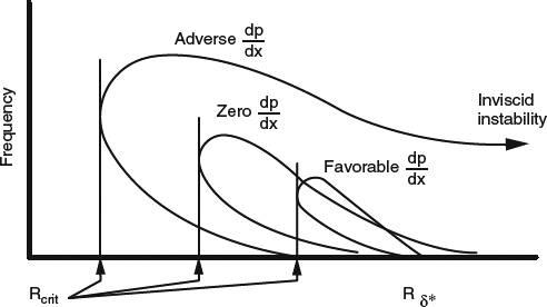
Figure 4.4.3 Schematic illustration of neutral stability boundaries for 2D (TS) disturbances in laminar boundary layers with favorable, zero, and adverse pressure gradients

Disturbance growth of the kind predicted by linear stability theory is well established as part of the natural-transition process in boundary layers and planar 2D channels, but not in all “thin” viscous shear flows. Flows in circular pipes are unconditionally stable according to the theory, and yet there is still an upper limit to the Reynolds number at which laminar flow can exist. Why the theory doesn't work for pipe flow is not understood.

Predictions of the stability theory for a flat-plate boundary layer (the neutral-stability boundary and the frequencies of amplified disturbances) were convincingly verified in a wind tunnel with very low turbulence levels at the U.S. Bureau of Standards in about 1940, but the results were not published to the international aerodynamics community until after World War II (Schubauer and Skramstad, 1947). The eⁿ transition-prediction method was first developed in the early 1950s (Smith and Gamberoni, 1956; Smith, 1981), and it was not until the 1970s that computers and solution algorithms progressed to the point that the spatial stability problem could be routinely solved for arbitrary pressure distributions.

The eⁿ method involves marching in the direction in which disturbance growth is assumed to take place (the flow direction in 2D flows), and at each station solving the stability equations for a range of different modes to determine the growth rates. Then the growth rates are integrated in the growth direction to determine the amplitude ratio A/A_o (the ratio of the disturbance amplitude to the initial amplitude at the station where the first instability appeared). The initial and final amplitudes themselves are not explicitly determined, only the ratio. This is usually expressed as ln(A/A_o), which is just n in the expression A/A_o = eⁿ.

The integration is carried out with differing degrees of rigor in different versions of the method. The rigorous choice is to do the integration for only one mode at a time as it evolves downstream, and to repeat the integration for a number of different modes covering the range of interest so as to determine at each station which one has produced the largest amplitude ratio. This generally means covering a two-parameter space, varying both β and ω, which is laborious. A shortcut is to repeat the integration only for multiple values of ω, using the value of β at each station that gives the most-rapid growth. The choice of β can be simple for incompressible flow because β = 0 (wave fronts perpendicular to the flow) usually leads to the fastest growth, but in transonic flow a range of β must generally be searched. Arnal and Casalis (2000) call this the “envelope method” because the resulting curve of n versus x is the envelope of multiple curves for different values of ω. A further shortcut is to use the value of ω that yields the maximum amplification rate at each local station as input to the integration. I would call this the “locally most amplified” method. For general flows, these shortcuts have no physical basis, but they save computing time because they don't require generating as many stability solutions. Of course such shortcuts produce higher n factors at transition than a rigorous integration would. While this is compensated for by calibration, the lower physical fidelity of the shortcut methods should presumably result in greater scatter in correlations with experiments.

Whether shortcuts are used or not, an eⁿ calculation determines a value of n at each station that is supposed to reflect the cumulative growth of the most-amplified disturbance. Transition is predicted to take place when n passes a threshold value determined by calibration against similar flows for which the transition location is known. The threshold value of n thus accounts empirically for the receptivity phase and the final nonlinear growth and breakdown. In principle, it can account for such factors in the initial-disturbance environment as freestream turbulence level and surface imperfections, but only if the calibration database includes flows in which these things were varied. In the variable-n-factor method, it is possible to base the calibration on results from more than one type of experiment. For example, the primary calibration would come from a flow similar to the target application, and data from other experiments could be used to adjust for other factors, such as surface roughness.

In 3D flows with cross-flow, TS and CF disturbances are treated as independent, in keeping with the linearity of the theory. There are several strategies for keeping track of the range of disturbance modes of both types (see Arnal and Casalis, 2000). The one that seems to produce the tightest correlations with experiments tracks separate n factors for TS and CF, and transition is predicted by whichever crosses its particular threshold first. Unless the surface is extremely (impractically) smooth, it is important to use a variable n-factor to account for the effects of surface roughness on the CF disturbances (see Crouch and Ng, 2000; Crouch, 2008). Data are available for flows with a wide variety of disturbance-growth progressions, leading to transition by TS growth in some cases and CF growth in others. For flows with low freestream turbulence and very smooth surfaces, typical threshold values are e⁸ for TS transition and e⁶ for CF. A formula relating n_CF to roughness height is given by Crouch and Ng (2000), and one relating n_TS to freestream turbulence level is given by Mack (1977).

Methods have been developed that carry out the eⁿ method by interpolating tables of precalculated growth rates instead of calculating solutions to the stability equations, saving orders of magnitude in computing time. For 2D flows with TS transition only, the ISES and MSES codes (Drela and Giles, 1987; Drela, 1993) use a two-parameter table-lookup scheme that returns growth rates as functions of the boundary-layer parameters R_θ and H. At each local station, the fastest-growing disturbance is used (as a function of ω), so that this is analogous to a “locally most amplified” method. A similar scheme that handles both TS and CF was developed by Crouch, Crouch, and Ng (2001). The TS growth rates used in this method are maximized locally with regard to β, but not with regard to ω, and multiple integrations are carried out for multiple values of ω. It is therefore analogous to an “envelope” method.

The final stage of nonlinear growth and breakdown is complex, and the details probably vary depending on the nature of the disturbances that feed it, and on local conditions such as pressure gradient and freestream turbulence. In a flat-plate boundary layer, Emmons spots like the one shown in Figure 2.1d form randomly and grow wider, merging together until the entire width of the surface is covered by turbulent flow.

4.4.2 Turbulent Boundary Layers

The turbulence in a fully turbulent boundary layer is inherently 3D and is random in space and time. But being random doesn't mean it's a featureless jumble of random swirls. Boundary-layer turbulence contains a variety of coherent structures over a range of length and time scales, from small structures that are characteristic of the region close to the wall to larger structures that span more of the full thickness of the boundary layer. Such structures form at essentially random locations over the surface and at random times, and even for structures of a particular type, there is wide variability in detailed evolution from one instance to another. But structures with distinctive features show up with surprising regularity. Many of their characteristics follow fixed statistical distributions.

Statistical distributions (probability distribution functions) for flow quantities within the structures are anchored in their vertical positions by the wall, and the vertical extent of the larger ones scales roughly with the boundary-layer thickness. In the horizontal directions there are probability distribution functions that move with the structures and reflect their typical shapes and sizes. And horizontal positions of structures relative to each other aren't completely random. There are two-point correlations that reflect “typical distances” and “typical cycle times,” as well as “typical life spans” (paraphrased from Spalart, 2009, private communication).

Figure 2.1e shows flow visualizations of large eddies that appear in the outer part of the layer and illustrates how they differ in favorable and adverse pressure gradients. In these photos, the turbulence is made visible by smoke that was introduced through a slot in the wall upstream. The smoke has been transported away from the wall mostly by turbulent convection and has been diffused relatively little by molecular action, and it therefore tends to “mark” the turbulent, vortical regions. The regions empty of smoke are essentially nonturbulent and nearly irrotational, and we see that such regions can penetrate deep into the boundary layer. The boundary between turbulent and nonturbulent flow is highly convoluted but surprisingly sharp. As the structures move along with the general flow, the turbulence seen at fixed points in space in the outer part of the layer is intermittent in time. These large structures tend to scale with δ, the overall thickness of the layer.

The main smaller structures that appear in the inner part of the layer are associated with streamwise vortices. A pair of counter-rotating vortices is often linked in the form of a horseshoe, as shown in Figure 4.4.4. Where the flow between two vortices is downward toward the wall, higher speed fluid is carried toward the wall in what is called a sweep, and where the flow between two vortices is upward, lower speed fluid is carried away from the wall in a burst. The resulting streaky structure very close to the wall was shown in Figure 2.1f.

These turbulence structures have been studied intensively, both experimentally and by DNS. Comprehensive surveys are to be found in Robinson (1991) and Moin and Mahesh (1998). Surprisingly, this knowledge of organized structures has had very little effect on the practical prediction of turbulent boundary-layer flows. The reasons for this have to do with the nature of the turbulence modeling problem, which we've already discussed in Section 3.7. In the RANS equations (Reynolds-averaged Navier-Stokes) governing the mean flowfield, the turbulent transport of momentum is represented by the Reynolds stresses, which are local (single-point) averages of fluctuating velocity components. Of course, the Reynolds stresses in the real world reflect contributions from the organized structures, but for modeling purposes, incorporating information about organized structures into single-point averages is difficult. As a result, such information that has found its way into the turbulence models has been of a very low-order variety, such as the idea that the motions that matter have length scales that decrease with decreasing distance from the wall, which was around long before we gained our current awareness of coherent structures. So as interesting as organized turbulence structures are, our detailed knowledge of them has not had much influence on engineering practice. Of more practical interest are the mean velocity profiles and the strategies that turbulence models have used for predicting them.

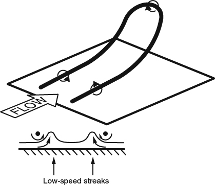
Figure 4.4.4 Pair of streamwise vortices forming a horseshoe pair in the inner part of a turbulent boundary layer

Typical mean velocity profiles in 2D turbulent boundary layers are illustrated in Figure 4.4.5. The most striking feature of turbulent profiles compared to laminar profiles is the very large velocity gradient at the wall. The highest gradient occupies a very thin region adjacent to the wall, too thin to be resolved on the scale of these plots. It is called the viscous sublayer because the shear stress there is effectively all viscous, with practically no contribution from Reynolds stress (see Section 3.7 for a discussion of Reynolds stress). But this lack of turbulent shear stress doesn't mean there is no turbulence in the sublayer. The flow in the sublayer is actually quite turbulent, with velocity fluctuations that are not small relative to the mean velocity. The Reynolds stress is nearly zero throughout a layer of finite thickness, not because the turbulence has disappeared, but because of the way the nearby wall constrains the turbulence, as we'll see next.

So the existence of the sublayer gives a distinctive appearance to turbulent mean velocity profiles. It also plays a vital role in the greater separation resistance of turbulent boundary layers relative to laminar, an issue we discussed in Section 4.1.4. There we noted that for a boundary layer to resist separation, fluid parcels near the wall must experience a favorable net viscous force associated with a positive shear-stress gradient ∂τ/∂y. In a constant-property laminar boundary layer, ∂τ/∂y = μ∂²u/∂y², and the favorable viscous force thus requires positive ∂²u/∂y². In the laminar case, the force is typically weak because μ is small. In a turbulent boundary layer, the rapid increase in the turbulent eddy viscosity outside the sublayer can provide a strong positive ∂τ/∂y even though ∂²u/∂y² is strongly negative there. One way to think of the turbulent boundary layer's greater resistance to separation is to imagine the strongly mixing part of the flow pulling the top of the sublayer along, keeping the velocity-profile slope and the skin friction positive.

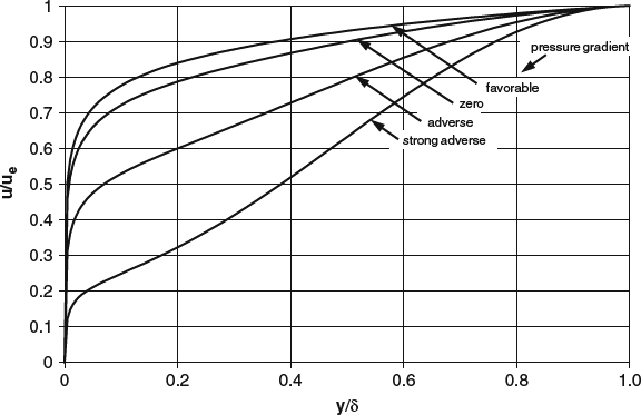
Figure 4.4.5 Typical mean-velocity profiles in 2D turbulent boundary layers in various pressure gradients

In much of the earlier literature, the sublayer was called the “laminar sublayer,” which wrongly implied that the flow in the sublayer is laminar. This unfortunate terminology has led to some misunderstandings, for example, in discussions of the effects of surface roughness, as we'll see in Section 6.1.8. It is clear from turbulence measurements and from flow visualization of the streaky structure in the sublayer in Figure 2.1f that the flow in the sublayer is anything but laminar. A closely related bit of misleading older terminology refers to the layer just outside the sublayer as the “buffer layer,” implying that it somehow buffers “laminar” flow in the sublayer against disturbances from outside.

Many discussions of how the Reynolds stress decreases as the wall is approached use the term “damping” in one way or another. For example, Van Driest (1956) developed a successful and subsequently much-used formula for the eddy viscosity that includes a “damping factor” (see Section 3.7 for a discussion of the concept of eddy viscosity), and Mellor and Gibson (1966) speculated that the sublayer and part of the “buffer layer” constitute a region in which “all disturbances are damped.” The term is not entirely inappropriate, in that the combination of viscosity and the no-slip condition at the wall does have a strong damping effect on the turbulence in this region, but it is potentially misleading because it suggests that the reduction of the Reynolds stress is due simply to a general reduction in turbulence level. The way that the Reynolds stress decreases as the sublayer is approached is actually more complicated than that.

The Reynolds stress of interest in a 2D boundary layer is and thus dependent to the same degree on both v′ and u′ velocity fluctuations. DNS simulations by Spalart (1988) show that the rms u′ level goes to zero linearly with y, pretty much across the entire sublayer. If v′ did the same, we might expect that would go to zero as y², and that there wouldn't be much of a seemingly finite sublayer. But rms v′ goes to zero much faster (as y²) than u′, and goes to zero as y³. So the Reynolds stress disappears faster than rms u′ in the sublayer and buffer layer because rms v′ disappears faster.

So why does rms v′ disappear faster than u′ near the wall? Both are constrained to be zero at the wall, so the answer isn't just in the boundary conditions. At least part of the explanation has to do with the length scales of the turbulence structures and how viscosity affects motions with different scales. If l is the typical horizontal (x or z) distance over which instantaneous u′, v′, and w′ vary, and given that u′, v′, and w′ obey the continuity equation, we can make the following loose statement about how the magnitudes of u′ and v′ are related:

So for motions with length scales much larger than y, v′ will tend to be much smaller than either u′ or w′, and there won't be much contribution to the Reynolds stress. The “active” motions (the motions that contribute to the Reynolds stress) tend to have length scales proportional to y, with v′ of the same order as u′. But viscous damping has an increasing effect as l decreases, and as we enter the buffer layer the intensity of motions with length scale l ∼ y decreases. If we think of viscosity as imposing a lower cutoff on l (an oversimplification, but with a grain of truth to it), we would expect v′ to decrease as y² while u′ decreases as y, as was observed in the DNS simulations.

Outside the viscous sublayer, we find another distinctive feature of turbulent velocity profiles: the pronounced “corner,” in which the second derivative of the velocity has a large negative value. In this region, the eddy viscosity increases rapidly with increasing y, and the velocity gradient diminishes accordingly, to the much lower levels typical of the outer part of the layer.

An interesting difference between turbulent and laminar profiles is in the appearance of inflection points in adverse pressure gradients. In our discussion in connection with Equation 4.2.7, we noted that in an adverse pressure gradient ∂²u/∂y² must be positive at the wall and that a laminar profile must therefore have an inflection point somewhere away from the wall. The same applies to turbulent profiles, but the inflection isn't generally visible in profile plots like Figure 4.4.5. Deep in the sublayer, ∂²u/∂y² must be positive, but just outside the sublayer it is strongly negative, and the location of the inflection point must be in the buffer layer, too close to the wall to be visible in ordinary profile plots. But inflection can also appear farther out in the profile. As indicated in Figure 4.4.5, a region of positive second derivative can appear in the outer portion of a 2D turbulent velocity profile if the pressure gradient is very strongly adverse or has been adverse over a long distance. Because the velocity profile tends to retain a pronounced negative second derivative both in the “corner” and near the edge of the boundary layer, a region of positive second derivative in the middle generally requires two inflections, as seen for the strongest adverse-pressure-gradient case in Figure 4.4.5.

Many of the available turbulence models can predict these distinctive features of turbulent velocity profiles, but before CFD became commonplace an understanding had already been developed based on physical reasoning, dimensional analysis, and simplified models. The physical reasoning starts with the idea that the boundary layer can be divided into an inner region and an outer region, and that in each region the velocity profile depends on the flow conditions in a distinctive way.

At the very bottom of a laminar boundary layer, the velocity profile is nearly linear and depends only on the wall shear stress and the viscosity, and not directly on the pressure gradient or on anything that happens in the outer part of the layer. In a turbulent boundary layer, the same dependence applies reasonably well to the wall region, which spans the viscous sublayer and the “corner” region of the velocity profile. To express this dependence in dimensionless form, we first define dimensionless wall variables:

where

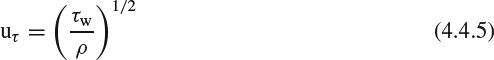
is called the friction velocity, and a unit of y⁺ serves as a length scale often called a wall unit. The dependence we're assuming, that is, that the velocity profile depends only on the shear stress and the viscosity, then takes the form of a basic functional relationship called the law of the wall:

In the viscous sublayer, the velocity profile is nearly linear, as it effectively is at the bottom of a laminar boundary layer, and f takes an especially simple form:

Farther out in the wall region, turbulent shear stress comes to dominate relative to the viscous shear stress. But the velocity profile still depends on the viscosity because the presence of the viscous sublayer has a large effect on the profile shape well into the part of the region where the turbulent shear stress has taken over. Shortly, we'll determine what functional form f must take in the outer part of the inner region.

In the outer region, we assume that momentum transport is entirely turbulent and that the velocity profile has no direct dependence on viscosity. The velocity profile in the outer region goes to u_e at the outer edge of the boundary layer and must merge with the wall-region velocity profile somewhere in the neighborhood of the “corner” of the profile. The remaining physical arguments regarding the outer-region velocity profile then go as follows. The outer region is like a boundary layer with a “slip velocity” at the wall, the slip velocity just being the velocity provided by the wall-region profile. The processes (primarily large eddies) that determine the velocity profile in the outer region don't “know” how much slip velocity is being provided by the wall-region profile, only how much shear stress is being transmitted, which is assumed to at least scale with the wall shear. Because the flow in the outer region doesn't “know” what its velocity is relative to the wall, the velocity that matters is the velocity defect, u_e – u, and the outer region is therefore often called the defect layer.

The velocity-defect profile is assumed to depend on the overall thickness δ of the boundary layer, the wall shear stress, the pressure gradient, and upstream history, but not directly on the viscosity. Expressing this in dimensionless form, we have

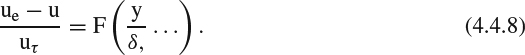
In a flat-plate flow, F depends only on y/δ because there is no pressure gradient, and upstream history effects are negligible because the shape of the profile is changing slowly. Equation 4.4.8 is then known as the velocity-defect law, and data from many experiments on both smooth and rough walls closely define a single function F, provided R_θ is above about 6000. Then there is the special class of flows that we've already noted known as the equilibrium turbulent boundary layers, in which the pressure-gradient parameter β defined by Equation 4.3.8 is constant in x. In an equilibrium turbulent boundary layer, the function F is also constant in x, but with a different function for each value of β, as we discussed previously in connection with Equation 4.3.9. Equilibrium boundary layers were first described by Clauser (1954, 1956), and further theoretical issues were investigated by Mellor and Gibson (1966). For more general cases, F is not universal, but the important thing for our purposes is that the defect profile is a function of y/δ and not directly a function of viscosity.

So we have inner and outer regions in which the velocity profile has different kinds of functional dependence. The final physical argument in this analysis is that there is a significant overlap region in which both kinds of dependence (Equations 4.4.6 and 4.4.8 hold. In the overlap region, we then have

The velocity profile thus is given by a function f of y/δ multiplied by a constant, and at the same time by the function F(y/δ) with a constant added to it. As first pointed out by Millikan (1938) (see also White, 1991), the only possible functional form is logarithmic. The resulting logarithmic law of the wall for the overlap portion of the inner region is usually written

where κ is called the von Karman constant and has been assigned values between about 0.38 and 0.44 depending on what experimental data are used. The constant B also varies depending on what value of κ was chosen, among other things. It is typically about 4.9 for a smooth wall and is smaller when the wall is rough, as we'll see in Section 6.1.8. The logarithmic overlap typically extends from y⁺ ≈ 0 out to about 0.15δ. At very high Reynolds numbers, the sublayer is very thin, and the log profile occupies nearly the whole region from the wall to 0.15δ, while at the lowest Reynolds numbers at which turbulent flow can be sustained, the log profile disappears.

Outside the viscous sublayer, the velocity profile blends smoothly from the linear sublayer profile to the log profile. Spalding (1961) devised a composite formula that fits the entire law-of-the-wall region:

which is illustrated in Figure 4.4.6. There are not many reliable sets of experimental data defining the profile in this region, but this formula fits the available data well (see White, 1991).

Why does it matter that a portion of the typical turbulent velocity profile is logarithmic? Well, there are at least two practical applications for this bit of knowledge. One is that surface roughness causes a shift in the logarithmic profile, and the shift provides a practical way of characterizing the effect on the skin friction, making it possible to take empirical roughness data from one flow situation and apply them to other flow situations, as we'll see in Section 6.1.8. Another is that the logarithmic profile provides a way to determine C_f from experimental measurements of the mean velocity profile. The viscous sublayer is typically so thin that measurements can't be made close enough to the wall to determine ∂u/∂y directly, but the logarithmic part of the profile can often be measured reasonably accurately. So in principle we should be able to determine the value of C_f that makes the measured profile fit the logarithmic law best. Clauser (1956) proposed one very effective way of doing this. First, recast Equation 4.4.10 in terms of C_f and u_e:

a form of the log law in which increasing C_f increases both the slope and the intercept. Then all we have to do is to plot Equation 4.4.12 for an array of closely-spaced values of C_f and plot the measured profile in terms of u/u_e versus log(y u_e/v) for comparison. Figure 4.4.7 illustrates how this works. The portion of the experimental profile that is logarithmic is easily identified, and the curve it lines up with best provides an estimate of C_f. This kind of plot is often called a Clauser plot.

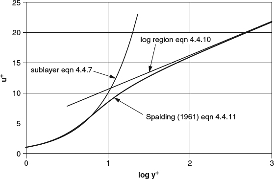
Figure 4.4.6 Velocity profile in the law-of-the-wall region of a turbulent boundary layer

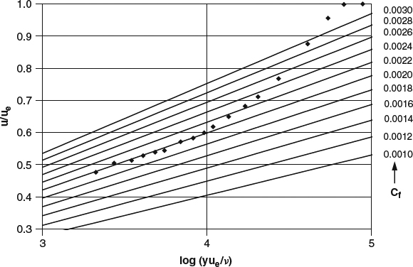
Figure 4.4.7 A “Clauser plot” of an experimental turbulent velocity profile compared with curves plotted from Equation 4.4.12, showing how an experimental estimate of C_f can be made (C_f ≈ 0.0020 in this case). (Data from McLean, 1970; for a case about halfway between the onset of an adverse pressure gradient and separation)

The velocity-defect form in Equation 4.4.8 isn't very convenient for general flows because the function F isn't universal. Coles (1956) found another way of representing the outer-region velocity profile, in which a single universal function suffices. Instead of referencing the velocity in the outer region to u_e, he referenced it to the outward continuation of the inner-region profile, the law of the wall. In this formulation, the entire profile can be expressed in a single formula:

where f is the law of the wall and can be expressed as a combination of Equations 4.4.7 and 4.4.10 or in terms of Equation 4.4.11, and the function W is well represented by

The constant Π is determined by the difference between the law of the wall and the actual velocity u_e at y = δ. The function W resembles the velocity profile in half of a turbulent wake and is therefore called the wake function, and Equation 4.4.13 is called the law of the wake. Equation 4.4.13 is compared with the same measured turbulent velocity profile used in Figure 4.4.7, first in terms of inner-region variables in Figure 4.4.8a, and then in terms of u/u_e versus y/δ in Figure 4.4.8b. This level of agreement with data is typical.

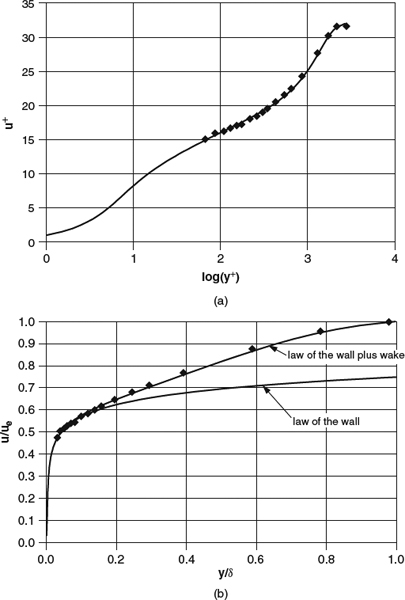
Figure 4.4.8 A typical experimental velocity profile compared with Coles' law of the wake. Same experimental data as in Figure 4.4.7. (a) In terms of wall variables. (b) Conventional velocity profile

The wake function W, shown in Figure 4.4.9, is “concave” (negative second derivative) in the bottom half and “convex” in the upper half, with an inflection point in the middle. Thus one component of the law-of-the-wake profile always has an inflection point, even when the pressure gradient isn't adverse. But the general convexity of the other component, the law of the wall, tends to keep the overall profile convex unless the adverse pressure gradient is strong or has been in force over a long distance. This can be seen in Figure 4.4.8b, in which the profile shown is in a moderately strong adverse gradient, at a station about half way from the onset of the pressure gradient to separation, and the profile is still convex, though just barely.

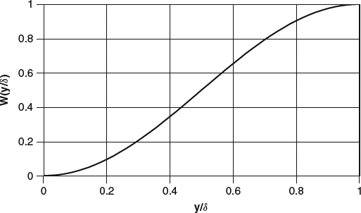
Figure 4.4.9 Wake function W(y/δ), defined by Equation 4.4.14, used in the law of the wake, Equation 4.4.13

The use of the word “wake” in the law of the wake is odd in a way. Coles (1956) noted the similarity of the function W(y/δ) to half of a wake velocity profile and proposed thinking of the outer part of a turbulent boundary layer as a half-wake. While a turbulent free wake and the outer region of a turbulent boundary layer are both regions of velocity deficit relative to u_e, the “wake component” 2Π W/κ of the law of the wake is, according to Equation 4.4.13, a velocity excess relative to the law of the wall. The entire law-of-the-wake velocity profile, including the law of the wall component, is often not at all wake-like in appearance, as, for example, in Figure 4.4.8b.

The skin friction is much larger for a turbulent boundary layer than for a corresponding laminar flow, as we saw for flat-plate flow in Figures 4.3.1–4.3.3. The difference between turbulent flow and laminar flow is even more dramatic when we look at it in terms of the eddy viscosity μ_t compared with the molecular viscosity μ. Away from the wall in a turbulent boundary layer, the mean-velocity gradient quickly becomes much smaller than it is at the wall, while the shear-stress level tends to remain high. This situation reflects levels of eddy viscosity that are orders of magnitude higher than the molecular viscosity. In Figure 4.4.10, we plot the ratio μ_t/μ for flat-plate boundary layers over a range of Reynolds numbers, according to the eddy-viscosity model of Mellor (1967). The μ_t/μ distribution in the inner region, plotted versus y⁺, is independent of Reynolds number, as shown in part(a). It is the linear-looking part of the μ_t/μ distribution that produces the logarithmic part of the velocity profile. The outer region eddy viscosity is proportional to R_δ* as seen in part(b), a relationship first suggested by Clauser (1956). In some models, for example, Cebeci and Smith (1974), the eddy viscosity decreases toward the outer edge of the boundary layer to account for the intermittency of the turbulence. Mellor and Gibson (1966) claim this makes little difference in the calculated mean-velocity profiles.

In Section 4.1.2, we discussed the distinctive aspects of 3D boundary layers in general terms: shear- and pressure-driven cross flow, cross-flow velocity profiles, direction profiles, the nature of separation in 3D, and the effects of cross flow on the flow development and the displacement effect. An additional complication arises in turbulent 3D flows, and that is that the relationship between the mean-velocity gradient and the shear stress becomes more complex.

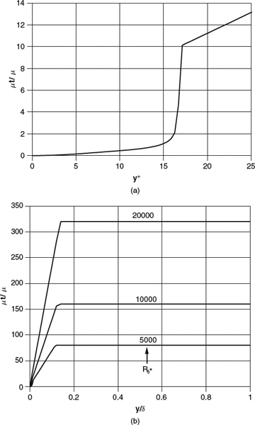
Figure 4.4.10 Levels of eddy viscosity given by Mellor and Gibson's (1966) model, for flat-plate boundary layers over a range of Reynolds numbers. (a) The inner region, in wall region variables, in which the variation is independent of Reynolds number. (b) Over the entire boundary-layer thickness, where the inner-region variation of (a) takes place too close to the wall to be visible

One way of looking at this relationship is to think of the shear stresses and the velocity gradients as vectors (τ_x, τ_z) and (∂u/∂y, ∂w/∂y) defining directions parallel to the surface. In 2D flows, these vectors are in the same direction, the direction of the entire flow, given by the vector (u_e,0). In 3D, the shear stress and the velocity gradient line up only in laminar flow or in the viscous sublayer of a turbulent boundary layer. In the turbulent part of a 3D boundary layer, they are generally skewed at an angle relative to each other, with the shear-stress direction often lagging behind when the velocity-gradient direction changes, as is the case in the example shown in Figure 4.4.11. Van den Berg (1988) compiled a list of possible physical mechanisms for the skewing, but what the mechanisms actually are in typical 3D boundary-layer flows has not been resolved.

The skewing means that the eddy viscosity has different values in the two directions, and it can have major effects on the development of the mean-velocity field. Many turbulence models ignore this, however, and assume that the eddy viscosity is isotropic (the same in all directions). We'll discuss this problem further in connection with the prediction of swept-wing flows in Section 8.6.2.

In most applications, we are not interested in the unsteadiness associated with a turbulent boundary layer, and we tend to measure or attempt to predict only the time-averaged (mean) flowfield. But the pressure fluctuations at the surface are sometimes important, as, for example, in the generation of boundary-layer noise. These tend to have broad-band spatial and temporal spectra reflecting the range of scales in the boundary-layer turbulence. In an attached boundary layer, the lowest spatial and temporal frequencies tend to be those associated with the passage of large structures such as those shown in Figure 2.1e. Boundary-layer separation from anywhere but a single, sharp trailing edge will give rise to lower frequencies associated with fluctuations of the instantaneous separation location and of the separated shear layer, and these fluctuations can be felt far upstream. Separation also increases the intensity of the surface pressure fluctuations, by something on the order of 10 dB, and reattachment of a turbulent shear layer increases them even more.

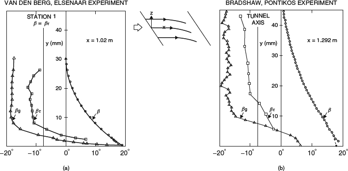
Figure 4.4.11 Examples of the skewing that can take place between the shear-stress direction β_τ and the velocity-gradient direction β_g compared to the outer-flow direction β in a 3D turbulent boundary layer in an adverse pressure gradient. See Bradshaw and Pontikos (1985). (a) Data from van den Berg, (1988). Published by AGARD. (b) Data from Bradshaw and Pontikos, (1985).

4.5 Control and Prevention of Flow Separation

As we noted in Section 4.1.4, delaying or preventing separation is important in many applications. In this section, we'll discuss some of the strategies that are used.

4.5.1 Body Shaping and Pressure Distribution

Separation from a smooth surface is generally related to a rapid or sustained rise in pressure, as we saw in Section 4.1.4. Thus a powerful means of delaying separation is through the shaping of the body so as to control the pressure rises. This usually means providing a generally streamlined shape, without sharp corners or large surface curvatures, and with a gradual closure at the back of the body to a sharp or almost sharp trailing edge or tail. If the closure is too abrupt, separation ahead of the tail will occur, as in Figure 4.1.2b or c. We'll consider the distinction between streamlined and bluff bodies further, as well as the underlying physics issues, in Sections 5.2, 6.1.3, 6.1.5, and 6.1.6. Even for a streamlined body, some fairly subtle details of the pressure distribution can be important. We'll consider this issue in some detail in connection with the maximum lift of airfoils in Sections 7.4.3 and 7.4.4.

Separation in 3D can form complicated flow patterns such as the necklace vortex separation that can occur in a wing-body junction, as shown in Figure 4.5.1a,b. A fillet or strakelet can eliminate the separation at the leading edge itself by easing the adverse pressure gradient and increasing the flow divergence ahead of the junction, as shown in Figure 4.5.1c. The change in the surface shear-stress pattern between (b) and (c) is dramatic. We should remember, however, that the surface shear-stress pattern tends to give an exaggerated impression of the change to the overall flowfield, as we pointed out in Section 4.1.2 and saw in Figure 4.1.11. Separations like the one in Figure 4.5.1b tend to be confined close to the body surface and to have very minor effects on the rest of the flow.

4.5.2 Vortex Generators

Generating streamwise vortices in the boundary layer upstream of where separation would otherwise occur can be an effective preventive measure. A vortex generator (VG) is usually a low-aspect-ratio vane with a planform ranging from delta to rectangular, attached perpendicular to the wall and placed at an angle of attack of about 15° to the local flow, so as to produce a strong vortex. The basic types are illustrated in Figure 4.5.2. A conventional VG is usually sized about as high as the boundary layer is thick (h ≈ δ), while a subboundary-layer vortex generator (SBVG) is much smaller . VGs are generally used in arrays and characterized by whether the vortices are all of the same sign (co-rotating) or of alternating signs (counter-rotating). In addition to vanes, various sorts of wedges, bumps, and scoops have been used to generate counter-rotating vortex pairs, but these devices are less common than vanes.

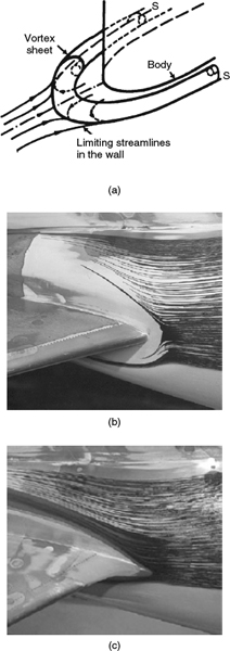
Figure 4.5.1 3D separation in a wing-body junction. (a) Sketch of a necklace vortex separation in a junction without a fillet. (b) Oil-flow photo of necklace vortex separation in a horizontal-tail junction. (c) Oil-flow photo of same junction as in (b) with strakelet installed

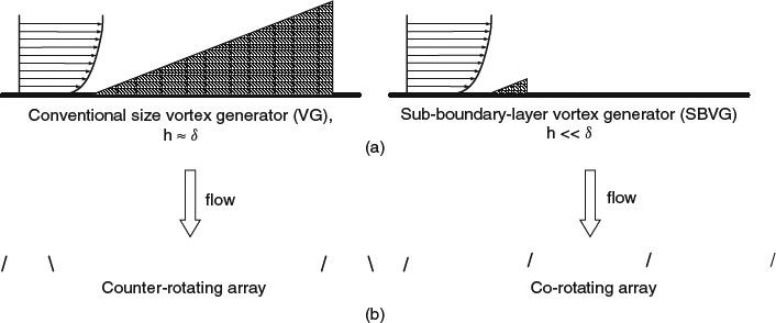
Figure 4.5.2 Types of vortex generators used for delaying or preventing separation. (a) Scaling of VG planform relative to boundary layer. (b) Arrangement of VGs on surface

A common explanation for the effectiveness of VGs is that they “enhance mixing.” We've seen that a turbulent boundary layer is more effective than a laminar one at resisting separation, and it seems logical that introducing more mixing would make it even more effective. There is an element of truth to this idea, but it is an oversimplification, especially in the case of conventional large VGs. What a large VG does to the flow can be looked at either in terms of a large side force “pushing” the flow strongly to the side, or in terms of “induction” by a strong vortex. Either way, the result is a major rearrangement of the mean-velocity field, as illustrated in Figure 4.5.3 in terms of streamwise vorticity and velocity contours in a cross-plane downstream of the VGs.

Counter-rotating VGs (Figure 4.5.2a, left side) produce bands of strong flow divergence (Figure 4.5.3a), where the boundary layer is thinned considerably, which increases its resistance to separation, alternating with bands of flow convergence, in which the boundary layer is thickened, and resistance to separation is presumably reduced. As the vortices “migrate” laterally, the bands of divergence widen, and the bands of convergence narrow, until pairs of vortices converge on each other and begin to rise from the surface, as can be seen in Figure 4.5.3a. As the vortices rise, they lift some of the low-energy air away from the wall, so that it contributes less to the tendency to separate. If an array of counter-rotating VGs is placed insufficiently far upstream of where separation wants to occur, separation will occur in the convergence bands. If the array is placed too far upstream, the converged vortex pairs will rise too far and lose their effectiveness. The placement of an array, relative to its spacing, is thus a balancing act. And note that in counter-rotating arrays, the vanes are usually grouped in pairs, as shown in Figure 4.5.2c, such that vortex convergence and liftoff are delayed farther downstream than they would be with uniform spacing.

Co-rotating VGs (Figure 4.5.2b, right side) also produce bands of divergence (thinning) and convergence (thickening), as in Figure 4.5.3b, but not nearly as pronounced as those produced by counter-rotation.

Figure 4.5.3 Rearrangement of the boundary-layer mean-velocity field by conventional VGs, shown in terms of streamwise vorticity contours and the u/u_e = 0.99 streamwise velocity contour at several streamwise stations. From Pauley and Eaton, 1988. Used with permission. (a) With counter rotating VGs. (b) With co-rotating VGs

Which type of array is more effective at preventing separation depends on several factors. Here is a brief summary of the pros and cons of the two types:

• Counter-rotating: A counter-rotating array can be more effective over short distances because of the strong divergence it can produce, but vortex merging limits the distance over which it remains effective. The effectiveness of a counter-rotating array can be seriously degraded if the vortices in a pair are not of equal strength (Pearcey, 1961), and counter-rotating arrays are thus not very tolerant of flow direction changes that unbalance the angles of attack of the vanes. And in 3D flows with strong cross-flow in the boundary layer, the two vortices in a pair behave differently, as explained below, which tends to favor a co-rotating array.
• Co-rotating: A co-rotating array will usually have lower nearfield effectiveness, but its effectiveness will persist farther downstream. And a co-rotating array is usually favored in cases with strong boundary-layer cross-flow.

Strong boundary-layer cross-flow has two main effects (Shizawa and Eaton, 1992): The vortices from VGs decay two to three times as fast as they would in a comparable 2D flow, and vortices of opposite rotation behave differently, as we mentioned above. When the main vortex from the VG has the same rotation as the background cross-flow vorticity in the outer part of the boundary layer, the vortex tends to diffuse more rapidly, as shown in Figure 4.5.4a, than it does when the vortex rotates in the opposite direction, as in Figure 4.5.4b. So flow situations with strong boundary-layer cross-flow favor co-rotating arrays with rotation as in Figure 4.5.4b. An easy rule to remember is that the force exerted by the VG should push the flow in the direction opposite to the direction of the cross-flow. This is important in the application of VGs to swept wings. We'll discuss swept-wing boundary layers in some detail in Section 8.6.2.

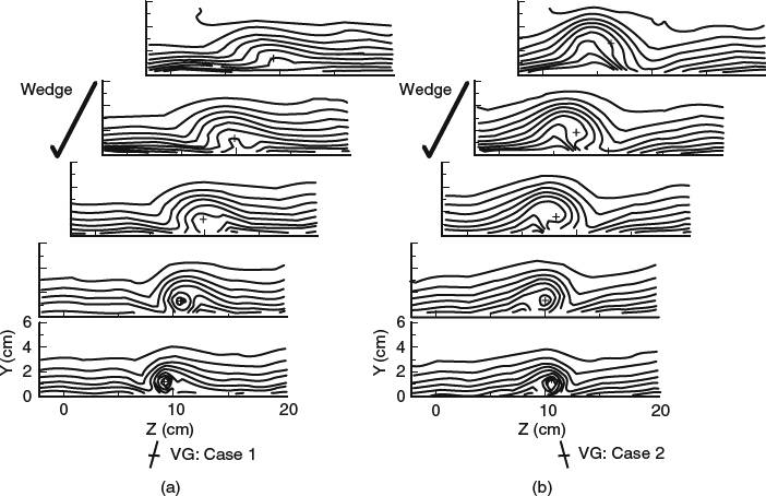
Figure 4.5.4 IIlustration of the effects of the direction of rotation of a vortex in a 3D boundary layer with strong cross flow, shown in terms of streamwise velocity contours. From Shizawa and Eaton, 1992. Used with permission. (a) Vortex rotation from a VG that pushed the flow in the same direction as cross flow near wall. (b) Vortex rotation from a VG that pushed the flow in the direction opposing the cross flow near wall

One of the most common applications for large VGs is to delay shock-induced separation on wings with transonic flow. The physical issues involved were discussed by Pearcey (1961) and ESDU (1993) provides installation design guidelines. Large VGs have also been used on fuselage closures, engine-inlet and wind-tunnel diffusers, and windmill blades (McMasters, Crowder, and Robertson, 1985). In general, counter-rotating VGs have been favored in flows that are without strong cross flow and in which the flow direction can be depended on to remain the same, and co-rotating VGs have been favored on swept wings.

For modeling the effects of VGs in CFD calculations, it's tempting to treat the flow only in a spanwise-averaged sense and to modify the turbulence model so as to simulate the effects of enhanced mixing. But we saw in Figure 4.5.3 that a boundary layer downstream of conventional large VGs has a pronounced large-scale spanwise-periodic structure, the effects of which are not likely amenable to averaging. The most successful modeling of large VGs so far has been based on 3D RANS calculations that resolve the individual vortices (see Yu, Kao, and Bogue, 2000).

SBVGs, on the other hand, are much smaller than conventional VGs and have spacings that are not so large relative to δ, so that it is much more reasonable to think of their effects in spanwise-averaged terms. The method developed by researchers at QinetiQ, Ltd, based on experimental measurements by Ashill, Fulker, and Hackett (2001, 2002), follows this general strategy in simulating the effects of SBVGs in a 2D integral boundary-layer code.

4.5.3 Steady Tangential Blowing through a Slot

Blowing air through a tangential slot in the wall can be a very effective way to delay separation. The air can be introduced passively through an open slot in an airfoil, as in Figure 4.5.5a, or actively from a pressurized air source, as in Figure 4.5.5b. In either case, the result downstream of the slot is a velocity profile of the wall-jet type, with a velocity peak near the bottom of the layer. Note that in the passive case the maximum total pressure in the jet is the freestream total pressure, so that the maximum velocity at the jet exit is about the same as the inviscid-flow velocity at the edge of the boundary layer. In the active case, on the other hand, total pressures substantially higher than freestream are typically used, which results in higher jet velocities. Because of the typically higher momentum flux, active blowing tends to be implemented with a narrower slot than passive blowing.

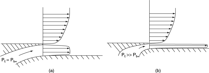
Figure 4.5.5 Tangential blowing slots and associated wall-jet velocity profiles. (a) Passive open slot. (b) Active slot with pressurized air supply

Much of what is known about the performance of wall jets in preventing separation applies to the active case with a relatively narrow slot and a high jet velocity. In this situation, the slot height and jet volume flux required to control downstream flow separation tend to be relatively small, so that the details of the jet velocity profile don't matter much, and performance depends primarily on the integrated jet momentum flux. On the other hand, a passive wall jet, with its larger slot height and lower jet velocity, is not so simple and does not seem to perform in a way that correlates neatly with simple flow parameters. Understanding passive slot blowing requires taking a different view, looking at the problem in terms of the boundary layers and pressure distributions on the individual surfaces rather than in terms of a single jet. We'll discuss this approach to understanding the passive slot effect in Section 7.4.4.

Steady slot blowing is a “brute force” method of separation control in that it works by providing the fluid at the bottom of the boundary layer with the additional momentum it needs to overcome a longer run of adverse pressure gradient without separating.

The usual correlation parameter for the effectiveness of high-velocity wall jets in preventing separation on an airfoil of chord c is the momentum-flux coefficient:

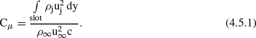
The level of C_μ required depends on how far separation needs to be delayed and on other details of the particular application. To bring about a major change in separation behavior, for example, to achieve fully attached flow on a plain (unslotted) trailing-edge flap at a large deflection angle, might require C_μ ≈ 0.02–0.06, depending on the details. Performance of slot blowing correlates reasonably well with C_μ in the sense that for a given airfoil shape and flow condition, performance is insensitive to slot height and jet velocity, provided C_μ is kept constant. Lachman (1961) and Korbacher (1974) survey an extensive assortment of early investigations of the overall performance of steady blowing in delaying separation, and McGahan (1965) made detailed flowfield measurements in a series of separating flows with steady blowing.

Steady blowing can be highly effective in delaying or preventing separation, but it tends to be costly in an energy sense. For most of the practical applications where blowing might be considered, providing a C_μ level above 0.01 requires a large amount of compressor power.

Providing slot blowing can entail other practical problems as well. An effectively 2D slot interrupts the skin of the body, and an alternative path for possible structural loads must be provided. And if the required slot height is small, maintaining the height accurately can be a problem, especially if the jet supply pressure is high. In some cases, an attractive alternative is to replace the slot with a spanwise array of discrete nozzles discharging parallel to the surface. Only discrete holes through the skin are then required, and precise nozzle geometry is easy to maintain. Discrete-jet blowing has been found to be just as effective as slot blowing, provided that the nozzle array is placed far enough upstream so that the discrete jets have a chance to merge sufficiently to prevent separation where it needs to be prevented (McLean and Herring, 1973).

4.5.4 Active Unsteady Blowing

Active unsteady blowing is a much more recent development than steady blowing, and it involves entirely different physics. Instead of preventing separation by brute force addition of momentum to the bottom of the boundary layer, unsteady blowing controls the effects of separation by manipulation of the separated shear layer. Unsteady excitation provided by a pulsed blowing jet or by a small mechanical flapper (like a miniature version of the spoilers used on wing upper surfaces) excites instabilities in the separated shear layer, causing it to oscillate with a large amplitude. The time-averaged flowfield that results is intermediate between the separated flow that would occur without control and the fully attached flow that could be achieved with sufficiently intense steady blowing. On an airfoil or trailing-edge flap, for example, the increment in lift relative to the separated case is less than what could be achieved with steady blowing but can still be substantial.

So unsteady excitation can't achieve the performance levels that steady blowing can, but there are indications that unsteady excitation can achieve useful levels with much lower energy inputs than required for steady blowing. For example, Seifert et al. (1993) reported substantial increases in C_{l max} for an airfoil with a plain flap deflected 30° with a time-averaged C_μ of 0.0006, roughly 2 orders of magnitude lower than steady blowing might have required. More recently, experiments and CFD simulations (the calculations by Shmilovich and Yadlin (2007), for example) have required much higher excitation levels, however. The excitation level that would actually be required to provide attractive performance for a real aircraft high-lift system is still highly uncertain.

There are two distinct approaches regarding the frequency of excitation. Earlier experiments on unsteady blowing (Seifert et al., 1993) found a relatively low reduced frequency of excitation fc/u_∞ ≈ 1 to be most effective. More recently, a high-frequency approach using frequencies an order of magnitude higher has been proposed (see Glezer, Amitay, and Honohan, 2003, for example).

4.5.5 Suction

Suction through slots or porous surfaces can be highly effective at delaying separation, essentially by removing the air with the lowest momentum at the bottom of the boundary layer and thus delaying the reversal of the velocity profile. Schlichting (1979) shows flow visualization images of slot suction delaying separation in a diverging channel and in the external flow around a circular cylinder. Thwaites (1958) shows experimental data for a circular cylinder on which porous-surface suction eliminated separation so that the theoretical potential-flow pressure distribution was nearly achieved. In Section 6.1.10, we'll look at another way of applying suction, in which the body shape is designed to localize all of the body's pressure recovery over a single suction slot, where a large fraction of the boundary layer arriving from upstream is removed. In practical applications, suction, like steady blowing, tends to be costly in terms of energy.

4.6 Heat Transfer and Compressibility

In our theoretical discussions so far in this chapter, we've generally assumed constant-property flow. Though the general momentum-transport processes and the development of the velocity field we've discussed so far wouldn't likely be changed qualitatively by variations in properties, variable fluid properties can have important quantitative effects on the flowfield, and there are situations in which the heat transfer and the wall temperature are of practical importance. Such effects can come into play through heating or cooling at the wall, or through the effects of compressibility, or combinations of these.

4.6.1 Heat Transfer, Compressibility, and the Boundary-Layer Temperature Field

When either heat transfer or compressibility causes a variation in temperature in the neighborhood of a wall, we have, by definition, a temperature profile and a thermal boundary layer. The development of the thermal boundary layer depends both on what goes on in the flowfield and on the thermal boundary conditions at the wall, where either the temperature, the heat flux, or a relationship between the two may be imposed by the thermal properties of the body and other aspects of the thermal environment.

As an illustration of the kinds of effects that can arise, consider a wing skin that is also part of a fuel tank. Fuel was pumped into the tank at a temperature close to the ambient temperature on the ground, and now the airplane is flying at high altitude, where the air is much colder. The fuel is being cooled by heat transfer that is driven by the temperature difference and regulated by the thermal conductivity of the fuel and the skin, and by the effective conductivity of the thermal boundary layer. The surface temperature adjusts itself to balance the transfer of heat from the tank with the transfer to the flow. The temperature difference that drives the heat transfer to the flow is the difference between the actual surface temperature and the adiabatic wall temperature, which is just the temperature the wall would reach in the absence of heat transfer, as, for example, if the wall were a perfect thermal insulator. At very low Mach numbers, the adiabatic wall temperature is just the static temperature of the flow, while at higher Mach numbers it reaches an elevated adiabatic recovery temperature because the kinetic energy of the flow is significant, and some of it is turned into heat in the boundary layer through viscous dissipation. We'll shortly consider a simplified theoretical estimate of the adiabatic wall temperature.

Other sources of heat flux (electromagnetic radiation, for example) can also affect surface temperature. The surface of a vehicle at rest in the sun can become quite hot to the touch, but the temperature will drop rapidly as flow speed increases. The net electromagnetic heat flux in this case is the difference between the absorbed part of the incoming solar flux (the part that isn't reflected), which is roughly fixed, and radiation from the body, mostly in the infrared. As the body is cooled by the flow, the net radiation into it increases somewhat because the outgoing infrared radiation is reduced, but the effective conductivity of the thermal boundary layer increases greatly with flow speed, so that the radiation overall becomes less and less of a player in the heat balance that determines the surface temperature.

Thermal boundary layers encompass wide ranges in the relative importance of the various effects. For example, if the Mach number is low, and heat transfer is driven by small temperature differences relative to the absolute temperature, the density and viscosity will be almost constant, and the flowfield will be affected very little by the heat transfer. In such cases, the heat is conducted and convected by the flow much as a passive contaminant would be. With larger temperature differences and/or Mach numbers, on the other hand, the changes in density and viscosity can have significant effects on the flowfield. In some flows, heat transfer dominates the thermal effects, while in others, heat transfer from the wall is insignificant, and compressibility is the only source of temperature differences. And many flows land between these two extremes.

4.6.2 The Thermal Energy Equation and the Prandtl Number

The thermal energy equation governs the temperature field and its interaction with the velocity and pressure fields (see Schlichting, 1979, for a detailed derivation). The equation expresses the balance between conduction and convection of thermal energy, and its conversion to and from kinetic energy by compression, expansion, and viscous dissipation. The equation gives rise to an important dimensionless material property, the Prandtl number:

where c_p is the specific heat at constant pressure, and k is the thermal conductivity. The Prandtl number appears in both the thermal conductivity and viscous dissipation terms in the energy equation (see Table 3.9.2) and measures the relative importance of viscous diffusivity and thermal diffusivity in the development of the velocity and temperature fields. Schlichting (1979) uses an order-of-magnitude analysis to arrive at a rough estimate of how the Prandtl number affects the relative thicknesses of the velocity and thermal boundary layers in laminar flow:

In gases, the Prandtl number is not far from 1, and the thermal boundary layer tends to be similar in thickness to the velocity boundary layer, as illustrated in Figure 4.6.1a. In liquids, the Prandtl number is typically orders of magnitude larger, and the thermal boundary layer tends to be much thinner than the velocity boundary layer, as illustrated in Figure 4.6.1b. Of course, in real situations the thickness of the thermal boundary layer also depends on the upstream history of the thermal boundary condition. For example, there can be situations in which a pronounced temperature difference is introduced at the wall well downstream of the start of the velocity boundary layer. The thermal boundary layer arising from such a change in boundary condition will be thinner than the velocity boundary layer until the temperature difference has had a chance to diffuse out into the flow, as illustrated in Figure 4.6.1c.

4.6.3 The Wall Temperature and Other Relations for an Adiabatic Wall

In many high-speed flow applications the wall boundary condition is very nearly adiabatic, and it is useful to be able to predict the wall temperature. Because the Prandtl number in gases is close to 1, we'll take as a starting point an energy integral derived independently by Busemann and Crocco (see White, 1991) for the special case of Pr = 1. If we further assume a perfect gas and an adiabatic wall, the boundary-layer thermal energy equation can be integrated, with the result that the total enthalpy is constant through the boundary layer:

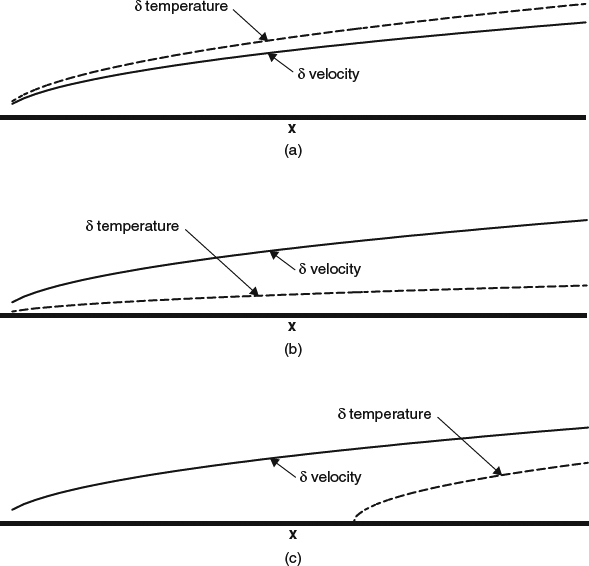
Figure 4.6.1 Schematic illustration of the thermal boundary layer in relation to the velocity boundary layer. (a) Gases (Pr about 0.7). (b) Liquids . (c) Gases (Pr near 1) after sudden change in wall temperature

Thus for Pr = 1, the adiabatic wall temperature, or the flow temperature at the wall, where u = 0, is the same as the stagnation temperature of the flow at the edge of the boundary layer, which in most external-flow situations will be the same as the far-field stagnation temperature.

But in gases the Prandtl number is a bit less than 1 (0.71 for air), and the adiabatic wall temperature is a bit less than the stagnation temperature at the boundary-layer edge. We define an adiabatic recovery factor:

We see that the Pr = 1 result of Equation 4.6.3 corresponds to r = 1. White (1991) presents approximate analyses indicating first that r should be very closely a function of Prandtl number only, and further that for laminar flow

and for turbulent flow

So we see that the adiabatic recovery temperature in air is much closer to the stagnation temperature than to the static temperature of the local outer flow, especially if the boundary layer is turbulent. These relationships should be good over the range of Prandtl number from 0.1 to 3.0, and provide a very convenient way to make rough estimates of the adiabatic wall temperature.

Consistent with the analyses that led to Equations 4.6.3–4.6.6, a reasonable approximation to the density and temperature profile for laminar or turbulent flow and an adiabatic wall is

where r is given by Equation 4.6.5 for laminar flow or Equation 4.6.6 for turbulent flow. A typical temperature profile for turbulent adiabatic-wall conditions according to this equation is illustrated in Figure 4.6.2.

The increase in temperature through the boundary layer is accompanied by a reduction in density, which increases δ* and reduces θ, so that the shape factor H is increased. Whitfield (1978) proposed a correlation for this effect for both laminar and turbulent flows up to M_e = 3, in terms of the kinematic shape factor H_K (H computed with the density ratio omitted from the integrals):

A plot of this relationship in Figure 4.6.3 illustrates how a given velocity profile with a given H_K results in significantly higher values of H at high Mach numbers. The increase in temperature also tends to reduce C_f. An approximation for this effect in the case of a flat plate was seen in Equation 4.3.7 and Figure 4.3.4.

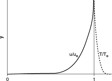
Figure 4.6.2 Velocity and temperature profiles for an adiabatic turbulent boundary layer in air at M = 1, according to Equation 4.6.7

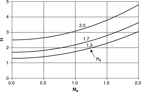
Figure 4.6.3 Effect of Mach number on the shape factor H for adiabatic-wall boundary layers, according to Equation 4.6.8

4.7 Effects of Surface Roughness

Distributed surface roughness can influence an aerodynamic flow in different ways depending on the situation: It can affect the location of laminar-to-turbulent transition, and it can alter the skin friction of a turbulent boundary layer and through combinations of these, it can alter the development of the boundary layer and the location of subsequent separation. In Section 4.4.1, we briefly discussed the effects of Reynolds number and roughness on transition, and in Section 6.1.6, we'll see how these can in turn affect the separation location and the pressure drag of spheres and cylinders. The maximum lift of an airfoil or wing also depends on separation, as we'll see in Section 7.4.3, so that roughness can affect maximum lift as well as drag. In Section 6.1.8, we'll look in some detail at how surface roughness can increase turbulent skin friction, which can influence total drag even when there is no change in transition or separation. This type of roughness effect is quite common in applications, caused, for example, by rough materials or paint, or by dirt or other contamination. Then in Section 6.2.2, we'll look at methods for using empirical data on roughness effects measured in simple flow situations for drag estimation in more-general flows. Riblets are an example of another sort of surface texture, one that would be applied purposely to reduce turbulent skin friction, and we'll discuss them in Section 6.3.2.