One of the chief challenges system or network administrators face is the ongoing task of maintaining optimal performance in a changing environment. The purpose of this chapter is to familiarize you with the various metrics, techniques, and strategies used to optimize performance, as well as the methodologies used to troubleshoot network, host, connectivity, and backup issues.

Optimize Performance

The principles and practices of storage optimization are the same whether it’s removable media such as portable hard drives, thumb drives, phone storage, or the large pools or arrays of storage that make up a large geographically dispersed storage area network (SAN). At the most basic level, performance optimization depends on factors such as the characteristics of the medium, including access speeds for read-write operations, its size, amount of used or available space, and type (sequential versus direct), as well as the way information is stored, indexed, or categorized.

Previous chapters introduced you to metrics such as recovery point objective (RPO), recovery time objective (RTO), and quality of service (QoS). All three are often understood within the context of recovery and business continuity when in fact achieving their target or best performance levels are tied, in part, to good storage optimization.

Necessary IOPS

One of the most basic metrics used in measuring storage performance is called input-output operations per second (IOPS). IOPS is used to measure how much data can be processed over a period of time, and it can be computed with the following formula:

IOPS = 1 / (average latency + average seek time)

For example, if a Serial Attached SCSI (SAS) drive running at 10,000 rpm has an average latency of 2.5 ms and an average seek time of 4.5 ms, you would take 1 / (.0025 + .0045), which gives you 142.857, or 143 IOPS rounded to the nearest integer.

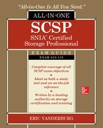
Table 12-1 provides typical IOPS values for devices. These numbers represent more of what you can expect rather than drive maximums listed on most sites.

Table 12-1 Typical Drive IOPS Values

A caveat should be noted when determining the true IOPS value of a given medium. Many manufacturers state values that are obtainable only in the most controlled or ideal circumstances. This practice is not unlike mileage per gallon (MPG) capabilities that auto manufacturers list when advertising vehicles. For example, Car X is listed with an MPG rating of 35 miles to the gallon on a highway. The weight of the driver, grade of gas, surface or condition of the road, installed options, and weather are just a few of the strictly controlled factors that few drivers, if any, will see on a consistent basis that will meet the target MPG rating. Similarly, true IPOS values will be impacted by the type of medium, access method, data management scheme, and amount of reserved or protected space needed to operate. Consequently, actual IOPS may be much lower than what is stated by the device’s manufacturer.

You can obtain IOPS metrics using a variety of tools, but one tool I recommend is IOMeter. It is free and available for both Linux and Windows. Figure 12-1 shows IOMeter’s dynamo command running on a local hard disk.

---

Figure 12-1 IOMeter dynamo command

Random vs. Sequential I/O

Random input/output access is usually used in environments such as databases and other general-purpose servers. In this access, all disks will be spending equal time servicing the requests. In simple terms, random access is seeking a random spot instead of retrieving data one bit after another on the disk. Caching and queuing can help reduce random I/O by allowing multiple writes to be saved to the cache and then written in a more sequential manner because the data can be written in a different order than the order it was stored in cache. The previous section introduced the concept of IOPS for reading and writing. There are also calculations for sequential and random IOPS.

There are several types of measurements related to IOPS: random read IOPS, random write IOPS, sequential read IOPS, and sequential write IOPS. Interestingly, flash-based media provide the same IOPS for random or sequential I/O, so these differentiations are used only for hard disk drives (HDDs).

•   Random read IOPS Refers to the average number of I/O read operations a device can perform per second when the data is scattered randomly around the disk

•   Random write IOPS Refers to the average number of I/O write operations a device can perform per second when the data is scattered randomly around the disk

•   Sequential read IOPS Refers to the average number of I/O read operations a device can perform per second when the data is located in contiguous locations on the disk

•   Sequential write IOPS Refers to the average number of I/O write operations a device can perform per second when the data is located in contiguous locations on the disk

RAID Performance

Storage professionals are often called on to create groups of disks for data storage. Grouping disks together allows for the creation of a larger logical drive, and disks in the group can be used to protect against the failure of one or more disks. Most grouping is performed by creating a Redundant Array of Independent Disks (RAID). RAID performance is contingent upon the type of RAID used, the size of the disks, and the number of disks in the RAID group.

RAID Type and Size

Several RAID specifications—called RAID levels—have been made. These levels define how multiple disks can be used together to provide increased storage space, reliability, speed, or some combination of the three. Although not covered here, RAID levels 2–4 were specified but never adopted in the industry; hence, they were never implemented in the field. When a RAID is created, the collection of disks is referred to as a group. It is always best to use identical disks when creating a RAID group. However, if different disks are used, the capacity and speed will be limited by the smallest and slowest disk in the group. RAID 0, 1, 5, and 6 are basic RAID groups introduced in the following sections. RAID 10, 0+1, 50, and 51 are nested RAID groups because they are made up of multiple basic RAID groups. Nested RAID groups require more disks than basic RAID groups and are more commonly seen in networked or direct attached storage groups that contain many disks.

RAID 1 is good for protecting against disk failure, but it offers poor performance. It is good for situations where few disks are available but good recoverability is necessary, such as for operating system drives. RAID 5 is good for sequential and random reads and fair for sequential and random writes. It is best used in database management systems (DBMSs) and for file storage. RAID 6 is good for sequential and random reads but poor for sequential and random writes. RAID 10 is good for sequential and random reads and writes. It is best used for online transaction processing (OLTP) and database management system (DBMS) temp drives.

The IOPS calculations introduced earlier can be applied to RAID groups as well as individual drives. Things get a bit more complex when RAID is factored in because the design of the RAID solution will impact whether it is optimized for read or write performance. Remember the calculation for IOPS provided earlier.

IOPS = 1 / (average latency + average seek time)

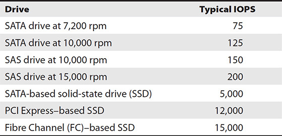
Read IOPS can be computed simply by multiplying the IOPS for a single drive by the number of drives in the RAID group. However, write IOPS is a bit different. To determine write IOPS for a RAID array, you must factor in the write penalty for different RAID types provided in Table 12-2. The reason RAID 5 has a higher write penalty is that parity must be computed. RAID 6 computes twice as much parity, so it has an even higher write penalty. Write IOPS is computed as follows:

Table 12-2 Write Penalties

Write IOPS = read IOPS / write penalty

Let’s consider some examples. A four-drive RAID 5 using SAS 10k drives would be computed as follows using the IOPS value from Table 12-1:

•   4 drives × 150 IOPS = 600 read IOPS for the RAID group.

•   Write IOPS would be 600 / 4 write penalty, or 150 write IOPS.

Now, consider the same four drives but in a RAID 10. Here, the read IOPS would still be 600, but the write IOPS would be 300 (600 IOPS / 2 write penalty).

You can see from these calculations that the type of drives and type of RAID utilized will impact the read or write IOPS available to applications running on logical drives from the RAID group.

Number of Disks

It is sometimes easy to think that more disks, often called spindles in this situation, in a RAID group will increase read and write performance, but there is a point where adding more disks can negatively impact write performance because of the number of parity computations necessary. Rebuild times also increase as more disks are added to the RAID group. Since RAID 10, RAID 1, and RAID 0 do not use parity, parity computations and rebuild times do not apply to them. Rather, it is RAID 5 and RAID 6 where you will need to consider parity and number of drives.

RAID groups that use parity include RAID 5, RAID 6, and the nested RAID groups RAID 50 and RAID 51. In such RAID groups, data is written to a collection of blocks from each disk in the RAID group called a stripe. The set of blocks in the stripe for a specific drive is called a strip, so a stripe is made up of strips from each drive in the RAID group. One strip in the RAID set is used for parity, while the others are used for data.

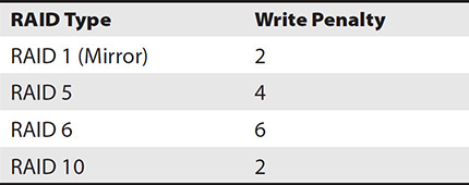
Parity is a value computed for a bit string by performing an exclusive OR (XOR) operation on two bits. The four possible XOR operations are listed in Table 12-3. When both bits are the same, the XOR is 0, and when they are different, the output is 1. For example, consider a five-disk RAID 5, which can also be referenced as 4+1, with 4 drives for data and 1 for parity. If the bit string in the first stripe is 1010, 0100, 0111, 1000, then you would XOR the first two stripes, 1011 and 0100, to get 1111. You then XOR that with the next strip, so 1111 and 0111 is 1000. Finally, you XOR 1000 with the fourth strip, 1000, producing 0000. 0000 would be written to the fifth strip in the stripe.

Table 12-3 XOR Table

The parity bit can be used to replace the data on a lost drive. In the previous example, the first bit string has 1010, 0100, 0111, 1000, and 0000. If disk 3 fails, you do your XOR operations again on the remaining disks to find the value for the missing one, XOR 0000, and the first drive, 1010, is 1010. This with the second drive is 1011 and 0100, equaling 1111. Now you take this and the fourth drive to derive the value for disk 3. 1111 and 1000 is 0111, which was the missing value on disk 3.

Our example computed and used parity to reconstruct the data for the first bit striped to the disks in this RAID 5 set. If you want to store 4MB of data on the RAID group, this data would be striped across four disks, so each disk would get 1MB, which is equivalent to 8 million bits since each byte has 8 bits in it and a megabyte has 1 million bytes in it. This 4MB file results in 8 million parity computations. The time it takes to process those computations and store their results is called the write penalty. For RAID 6, two drives are used for parity, so data must be written to both, increasing the write penalty.

As the number of disks grows in a RAID group, the number of bits that must be evaluated for a parity computation grows. Rebuilds, likewise, must evaluate more disks to determine which bit to write to the recovered drive. Rebuild times can be significant and can greatly impact the performance of a RAID group. These rebuild times can take several hours to several days depending on the speed of the drives and number of drives in a set.

Defragmentation

Defragmentation is a common method used to improve the performance of storage. Data and files are spread across disks as they are written, with each bit taking the next available location on the disks. This location is not always contiguous, with the previous bit resulting in more random reads instead of sequential reads as data gets more and more spread around the disk. Ideally, data should be placed on the disk such that the read-write head is positioned above it immediately after the previous bit of data was read from disk. When data is fragmented, the platter must rotate, and the head must be moved to a new location before the next bit of data can be read, which increases latency and access time, ultimately compromising the device’s performance. Defragmentation reorganizes the data so that it can be read sequentially to reduce latency and wear and tear on disks because of head and platter activity. For more information on how data is read from a hard drive, access time, and rotational latency, see Chapter 1.

To better understand the value of defragmentation as an optimization tool, think of a file cabinet. When the cabinet is properly organized, all of the folders are alphabetized, and the individual files are alphabetized as well. Suppose each time you retrieved a file within a given folder you replaced that folder at the front or end of the other folders. Over time this practice would result in folders being out of sequence, and files may or may not be in the appropriate folder. Additionally, the file may be in the correct folder but not in alphabetical order. The longer this condition is allowed to persist, the longer it will take you to find the folder and file needed. Defragmentation can be seen as a process where the folders and the files within them are realigned or sorted. Figure 12-2 shows the Windows Disk Defragmenter tool. Red bars show areas of the disk that are fragmented, and blue areas are files that are not fragmented or located on contiguous areas on the disk.

---

Figure 12-2 Windows Disk Defragmenter

Solid-state storage has a shorter use life when compared to hard drives because of the way it is constructed. Transistors called floating gates hold a charge to represent a binary 0 or 1. This value is changed by making the oxide layer surrounding it conductive. However, this can be performed only so many times before it breaks down. Since this change in conductivity happens each time there is a write or erase, the life span of the disk is tracked based on write/erase cycles. The average rating for single-level cell (SLC) SSD and multiple-level cell (MLC) SSD is 100,000 and 10,000 write/erase cycles, respectively.

Thus, the performance of SSDs is degraded each time data is accessed or written to it. Defragmenting or defragging SSDs does not result in any appreciable performance in enhancements. Consequently, defragmenting an SSD actually diminishes the life span of the drive by increasing the number of write cycles and results in no benefit.

Impact

Defragging involves the movement and relocation of a lot of data, which can significantly impact the performance of currently running operations and routines. Some defragging applications are dynamic in that they are able to determine the level of drive utilization or activity and adjust its process by slowing down when needed and resuming when it is not competing for I/O cycles. The result is that current processing speeds or performance is not compromised.

As previously mentioned, SSD drives do not benefit from defragging. There is no latency due to seek time because, regardless of where data is located, it takes the same amount of time to write or read data from solid-state technology.

Schedules

Most defragmentation operations can be scheduled during times when it will not hinder ongoing business operations and tasks. Additionally, defragmentation schedules can be automated so that storage can be optimized at a specified time and date without user or operator intervention.

Most storage media and defragging utilities are capable of automatic operation without the presence of a user or operator. The process of defragging competes with current I/O execution and may even result in a significant slowdown, so it is common to set up defrag schedules so that these operations do not occur during peak network or system utilization.

Cache

Cache is high-speed memory that can be used to service I/O requests faster than accessing the disk. Cache is referenced and organized by pages. Pages store data as well as a link to the location of the data on disk and a value called a dirty bit. The dirty bit is set to on when data is new or changed in cache, and this tells the controller head that the data needs to be flushed to disk.

In a storage environment, recently queried data, along with data that the system expects will be queried next, is stored in read cache, while data that is waiting to be written to the disk is placed in write cache. This allows the disk to function more independently from the interface so that one is not waiting on the other. The interface can load data into cache or read data from cache as it is received, and data can be written to the disk from cache or read into cache when it is optimal.

Read vs. Write Cache

Read and write cache are used to increase the speed at which data is retrieved or stored on an array. Read cache stores data from the disks in an array that the system anticipates will be requested. This speeds up requests for data if the data is resident in cache. Write cache is used to speed up the writing of data to an array, and there are two types of write cache, write-back and write-through cache. These three types of cache are described here:

•   Read ahead Read-ahead cache retrieves the next few sectors of data following what was requested and places that into cache in anticipation that future requests will reference this data. The read-ahead cache results in the best performance increase with sequential data requests, such as when watching videos, copying large files, or restoring files.

•   Write back Write-back cache sends an acknowledgment that data has been successfully written to disk once the data has been stored in cache but has not actually made it to disk yet. The data in cache is written to disk when resources are available. Write-back cache results in the best performance because the device is able to accept additional I/O immediately following the write acknowledgment. However, write back is riskier because cache failures or a loss of power to the disk could result in a loss of pending writes that have not been flushed to disk.

•   Write through Write-through cache waits to send an acknowledgment until a pending write has been flushed to disk. Although write-through cache is slower than write backup, it is more reliable.

Figure 12-3 shows the cache properties of a controller in an EMC array. Here, the read and write cache are enabled for both controllers, and the write cache is mirrored.

---

Figure 12-3 Storage array cache properties

An array that is used primarily for write traffic should have a large write cache to enhance performance, while one that primarily supports read traffic would benefit from a larger read cache. Storage administrators should understand the type of traffic they will receive and customize cache accordingly. Figure 12-4 shows how the read and write cache is allocated on storage array controllers.

---

Figure 12-4 Storage array cache allocation

De-staging

De-staging, or flushing, is the process of writing data from cache to disk. This process is usually performed when resources are available or when cache reaches an upper watermark, meaning that it is getting too full. De-staging is configured to start when the cache fills to a predetermined percentage or watermark. Figure 12-5 shows the cache de-staging properties of a Dell storage device. It is set to begin de-staging at 80 percent capacity.

---

Figure 12-5 Cache de-staging properties

Cache Hit and Miss

When a request is made for data that exists in the cache, it is known as a cache read hit. The storage array immediately services the request by sending the data over its interface without retrieving the data from disk. Cache read hits result in the fastest response time. When requested data does not exist in the cache, it is known as a read miss. It is a failed attempt for data to be retrieved from the cache memory. This results in longer access time because needed data must be fetched from the primary storage on the disk.

You can improve the cache read hit percentage by increasing the size of the read cache or by changing the read-ahead cache from least recently used (LRU) to most recently used (MRU), or vice versa (see Chapter 2 for more on LRU and MRU). As you can see in Figure 12-4, there is only so much cache available, so if you allocate more to read, you are taking it away from the write cache. It is important to evaluate your application needs so that you understand the number of reads and writes you can expect from the system. This will allow you to properly size the read and write cache.

Impact of Replication

Storage replication is the process in which the stored data is copied from one storage array to another. Replication can occur locally over a SAN or local area network (LAN) or to remote locations over a wide area network (WAN). In doing so, the reliability, availability, and overall fault tolerance are greatly enhanced. Replication allows for information, resources, software, and hardware to be shared so that they are available to more than one system. The significant benefits of replication include improving reliability and fault tolerance of the system.

Backup operations often use a local replica, called nearline storage, and a remote replica. The local replica may contain portions of the backups that are most recent, while more comprehensive backups are kept offsite. Sometimes the nearline and remote backups are identical. The advantage of this method is that restore operations can be completed in much less time than it would take to copy data from a remote backup site. Of course, the main reason for using a remote backup replica in the first place is to provide availability if the initial site goes down. In such cases, the organization would perform operations from the backup site or restore to another site from the remote backup replica.

Point-in-time (PIT) replicas can provide protection against corruption or changes in a system, and they are also used for litigation holds (see Chapter 11). However, this requires the system to keep track of all changes following the PIT replica, which can diminish performance.

Synchronous replication does not finalize transactions or commit data until it has been written to both source and destination. This form of replication is used for both local and remote replication scenarios. The major advantage of synchronous replication is that it ensures all the data remains consistent in both places. On the other hand, this type of replication can slow down the speed of the primary system since the primary system has to wait for acknowledgment from the secondary system before proceeding. If this is causing performance issues, you may need to consider upgrading equipment or switching to an asynchronous replication method.

Some enterprises use a combination of synchronous and asynchronous replication. Systems are often deployed using synchronous replication to another array at the same site, and then this array is replicated asynchronously to a remote site. This provides faster recovery and failover if a single array fails at the site than if asynchronous replication was used alone, while still providing recoverability if the entire site fails. See Chapter 9 for a review of synchronous and asynchronous replication.

The potential impact of several factors should be addressed when considering replication—latency, throughput, concurrency, and synchronization time. The impact these factors will have on a given storage environment is determined by the type of storage network. In a server-to-server or transactional environment, latency and throughput are the primary elements for optimization, while in an environment that uses merge replication, sync time and concurrency are the dominant factors. Overall care should be taken in balancing these factors, regardless of the type of replication deployed.

Latency

Latency is the time it takes to go from source to destination. In other words, it is the travel time, and it can have a significant impact on replication. Electrical impulses and light have a maximum speed. It may seem like light is so fast that latency would not matter, but it can have an impact at greater distances. Light travels at 186,000 miles per second in a vacuum and approximately 100,000 miles per second in fiber-optic cables. Therefore, it would take five milliseconds for light to travel 500 miles, the distance from New York to Cleveland, over fiber-optic cabling. Five milliseconds may not feel like much time for a human, but it can feel like a long time for a computer. Modern processors operate around 3 GHz, which equates to 3 billion cycles per second or 3 million cycles per millisecond, so a processor would go through 15 million cycles while the replica traveled 500 miles. Of course, sending replica data from one place to another is not as simple as dropping it on a wire. Devices forward or route the replica data to its destination along the way, and each of these devices will add latency to the equation.

Throughput

Throughput is a measure of the amount of data that can be processed over a link within a given interval or time period. In replication, the throughput between replica pairs must be sufficient for the data that will be transferred in order to avoid transmission errors, replica failures, or inconsistency between replicas. In some cases, initial replication may need to be performed on a different network or via direct-attached drives if throughput is insufficient. Further changes will then be replicated over the replica link.

Concurrency

Concurrency refers to the number of possible simultaneous replications that can be performed. This can especially be an issue as systems scale. For example, you implement replication between a data store and three remote offices. The offices synchronize with the central data store every five minutes. As the company grows, 15 more offices are added with their own replicas, but they have issues synchronizing because the central store can handle only five connections simultaneously. In such a case, it might make sense to upgrade the replication method to handle more concurrent connections or to create a replication hierarchy where not all sites replicate to the central store, but rather replicate to other hub sites, which then replicate back to the central store.

Synchronization Time

Synchronization time is the time interval it takes for data replication to be complete. Imagine the situation with the distributed system mentioned earlier. This system copies a local replica to each site, and users work from their replica, which is synchronized with the central data store. Imagine this is a product fulfillment system and a user from San Francisco orders a part from the warehouse for a customer and shortly thereafter a user from Boston orders the same part. This could cause a problem when the data is synchronized with the central data store if there is only one part in the warehouse, since both users were working from their local data store. In such cases, it may be necessary to decrease the synchronization time so that data is synchronized more often. It may also necessitate business rules to handle replication conflicts.

Partition Alignment

Partition alignment refers of the starting location of the logical block addressing (LBA) or sector partition. Maintaining partition alignment is essential in maintaining performance. Partitions can become misaligned when the starting location of the partition is not aligned with a stripe unit boundary in the disk partition that is created on the RAID. Data on misaligned partitions ends up being written to multiple stripes on the physical media, requiring additional write steps and additional parity steps. Partition alignment is a problem for SSD drives as well because it results in additional write cycles, decreasing the life span of the SSD.

With the growing use of virtualization, virtual hard disks can also suffer from partition misalignment where a virtual hard disk’s sectors are mapped between sectors on the physical media.

If you suspect that your partition is misaligned, compare the I/O requests made with the I/O requests processed. If the processed amount is significantly higher than the requests, you might have a partition alignment problem. You can also look at the offset of the partition using a tool such as sfdisk in Linux. The offset should be divisible by 8 or 16. Here is an example of a partition that is misaligned:

sfdisk -uS -l /dev/sda

This command executes the sfdisk utility with the -uS and -l switches. The -uS switch reports sectors in blocks, cylinders, and megabytes, while the -l switch lists the partitions of the device. We are performing this command on the /dev/sda partition. Here is the output:

This command shows that the first partition is misaligned because it is starting at 63. If it started at 64, the partition would be aligned, but this way it is starting one sector too early.

SSDs organize data into blocks and pages instead of tracks and sectors. SSD drives support LBA, so their storage is presented to the system as a series of blocks, and the controller board converts the LBA block address to the corresponding block and page. Partition misalignment must be avoided to minimize unnecessary reads and writes, which will not only result in performance degradation, but also shorten the life of the SSD.

Queue Depth

Queue depth is defined as the total number of pending input and output requests that are present for a volume. When the queue is full, there may be some lag time between the occurrences of server errors being reported by the presenting application. Too many pending I/O requests results in performance degradation. Whenever there is no space for any more requests, the QFULL condition is returned to the system, which means that any new I/O requests cannot be processed. There are several Java or alternative Internet-based sources for monitoring queue depth.

Each LUN will be allocated a section of the queue depth, and the amount of space allocated is dependent on the vendor. For example, some may have a total queue of 8,192 slots but allocate 64 slots for each LUN so the device can support up to 128 LUNs. This is important to know because it is tempting to think that 8,192 slots are available for the queue, but only 64 slots are available per LUN.

Some storage arrays and devices are equipped with Storage I/O Control (SIOC), which dynamically manages the queue depth, allowing for the controller on the storage unit to process commands in a way that is most efficient for it, such as processing data for two I/O requests that are in the same area of the disk. SIOC also throttles devices that try to dominate the queue to the exclusion of other devices, a problem that existed before queues were divided into sections per LUN. However, for the most consistency in performance, queue depths may need to be assigned manually for certain LUNs. For those who do not have SIOC and find queue depth is directly related to performance problems, it may make sense to split the data into multiple LUNs to take advantage of separate queues.

For example, one company had a virtual environment that went back to a single storage array. All their virtual machines ran off two 2TB LUNs that were mapped back to a RAID group on the storage array. They were experiencing performance issues, so we looked at a number of metrics. The queue depth was high for both LUNs. We allocated two new 1TB LUNs and split the machines from one of the 2TB LUNs between these two new LUNs. We then monitored the queue depth and saw a dramatic decrease and increase in performance, so the company allocated two more 1TB LUNs and removed the two original 2TB LUNs.

Storage Device Bandwidth

Storage device bandwidth is defined as the connectivity between the server and the storage device. The goal is to maximize the performance of or movement of data between the servers and storage devices in a given network. In this case, data transfer is enhanced, allowing applications to run at optimal speeds. There are a number of third-party utilities or applications to aid the system administrator in maintaining optimal bandwidth performance. Care must be taken in selecting the tools and strategy for managing storage bandwidth.

A balance must be struck between the increased complexity of applications and the costs of the storage networks they depend upon. This is especially true when multiple storage systems are interconnected. Load balancing is often problematic, as a vast number of geographically dispersed storage resources of different types and ages coexist in a network. Less-than-optimal load balancing will result in overutilization of some storage resources, while others in the network are grossly underutilized. Oftentimes new investments are made in storage to increase overall network performance when in fact better awareness and optimization would have addressed observed network performance issues.

If bandwidth is insufficient, consider adding more network cables and switch links or upgrading cables, NICs, and switches to versions with higher capabilities, such as moving from Gigabit Ethernet to 10 Gigabit Ethernet.

Bus and Loop Bandwidth

Bandwidth is how much data can be transferred during a measured interval such as a second, as in megabits per second. Whether the network is bus or loop, data transfers will utilize bandwidth and storage, and network administrators must be familiar with their application needs to determine whether the network links can provide the required bandwidth.

In previous chapters, we discussed the types of networks, and bus and loop were mentioned as compared to star networks. While bus and loop have predominantly been replaced by star networks, the bus and loop are still common within electrical systems such as circuit boards, and these systems differ from switched systems in the way contention for resources is handled.

A bus is a connection between two points. Typically, controllers or circuits will connect devices and manage the data that flows through the bus. In a parallel bus, traffic flows down multiple lanes in the bus simultaneously, as compared to the serial bus where data flows sequentially. Since a bus connects two points, the connection is dedicated to those points and contention is minimized. However, in the loop, traffic flows in one direction and must pass between multiple nodes in the loop to reach its destination. Each node in the loop receives an equal share of the bandwidth, and performance is predictable and reliable, but there is much overhead as data passes further through the loop than it would in a bus.

Both the bus and the loop are constrained by how much data can be transferred at one time. Storage administrators should be aware of the bandwidth available in system components so that they can understand where systems may be constrained. For example, imagine a storage system that is attached to a network with two 8 Gbps fiber connections. This system is upgraded to twelve 8 Gbps connections to handle additional servers that each issue a significant number of reads and writes (I/O). However, if there are only two 8 Gbps back-end ports for each disk shelf, the system may be constrained by the available back-end bandwidth.

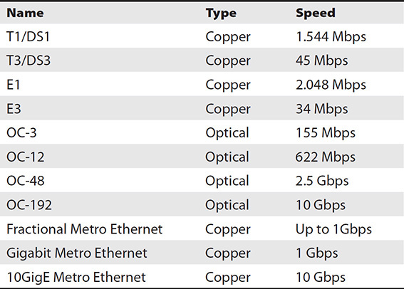
Cable Speeds

Cable speeds can impact performance. Cables are rated for a maximum speed, and they often perform at a rate much lower than their maximum. The applications in use will determine how much bandwidth is necessary. For example, streaming 1080p high-definition video at 24 frames per second might require 25–40 Mbps, and a business application streams a maximum of 10 concurrent videos at a time from storage over the WAN. This would require up to 400 Mbps of WAN bandwidth.

Ensure that the cables in use are adequate for your needs. LAN cables are typically Gigabit Ethernet such as CAT5e, but WAN connections may vary greatly. Table 12-4 compares a variety of WAN connections and their speed.

Table 12-4 WAN Connections and Their Speeds

Disk Throughput vs. Network Bandwidth vs. Cache

One big frustration for storage administrators is the inaccuracy of service requests made by users. The famous “system is slow” is one of my favorites because I have heard it so many times, and it provides almost no direction for the troubleshooter. In cases like these, you will need to investigate each part of the communication stream to determine where the slowness is occurring.

I/O commands start through an application that issues a command to the host bus adapter (HBA). Let’s explore a write command. The HBA determines the LUN the I/O write command is destined for and places it into a frame on the storage fabric. The frame travels through the fabric, possibly through one or more switches, and arrives at the storage array controller HBA. The controller receives the command, identifies the RAID group associated with that LUN, mirrors the command to other controllers in the unit, and writes the command to cache. It is up to the storage array to then send the command to the RAID controller, which sends individual commands to each of the disks in the RAID group, computes the parity, and writes the data to each stripe in the RAID group. In most cases, once the command is written to cache, the storage array can send an acknowledgment back through the storage array, over the network, and back to the host, which then sends it to the application. However, if many commands have been received and the disk throughput is not capable of keeping up, the command may have to wait for the cache to be flushed to disk before it can be processed.

As you can see, the process involves a lot of steps, and one or more of those steps could be contributing to the problem. It can be broken down into three states: network bandwidth, cache, and disk. Each of these elements can be measured in IOPS so that you work with the same data point for comparison’s sake.

Disk throughput can be measured by evaluating the rotational latency and interface throughput of the disk or storage array. In the case of SSD, rotational latency is not a consideration since SSDs do not have moving parts. Rotational latency is the amount of time it takes to move the platter, the round, flat surface inside an HDD where data is written, to the location of the desired data. Rotational latency is measured in milliseconds (ms). The interface is how the drive connects to the controller in a disk system such as IDE, SATA, and SAS (see Chapter 1 for more details).

Network bandwidth can be measured with different tools such as Cacti, Splunk, or PRTG network monitor, depending on where in the network you are evaluating the bandwidth. Each switch port will display its utilization on a managed switch. Simply connect to the switch’s management IP address and select the port you want to see, as shown in Figure 12-6.

---

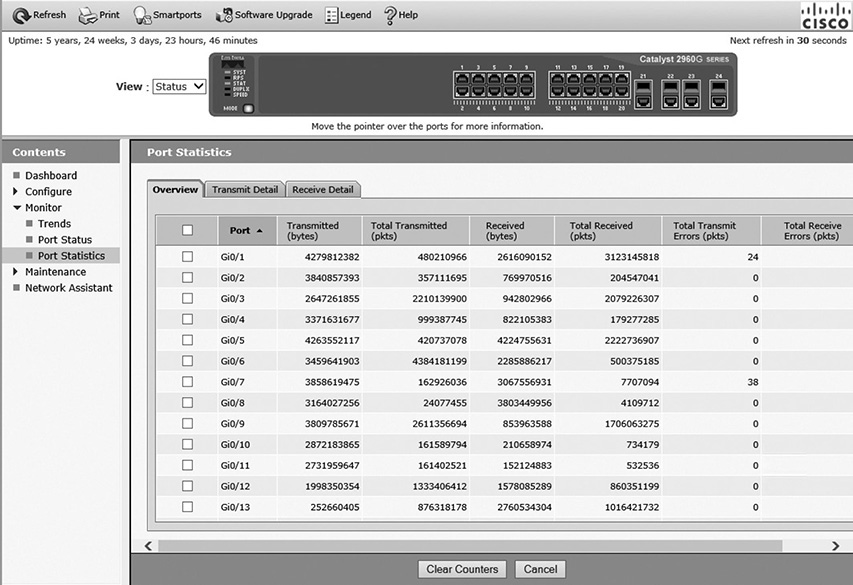
Figure 12-6 Bandwidth metrics from a switch management interface

A network interface card (NIC) in a computer can also display bandwidth statistics and sent and received packets. This can be useful to determine whether a switch port or NIC is saturated or underperforming. Figure 12-7 shows the statistics of a NIC on a Microsoft Windows client. SNMP and SMI-S–based management tools also offer a way to view statistics from a variety of devices such as switches, storage arrays, and other components.

---

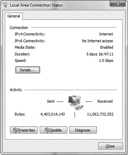
Figure 12-7 NIC statistics for Microsoft Windows client

Lastly, cache can be measured by reviewing the size and utilization of read and write cache along with cache read hits. This information can be obtained from command-line interface (CLI) or management tools provided by your storage vendor.

Embedded Switch Port Speed

In an embedded switch, all functions are performed at the chip level, resulting in increased reliability and overall performance. It is important that the device speed matches that of the cable and port to which it is attached. For example, if a port on the switch is rated or configured for 1 Gbps but the attached cable is rated lower, port errors will occur. These errors will result in the retransmission of the lost data along with the demand being made on the port by current data traffic. The devices, ports, and cables on the other end must also be capable of supporting the same speeds.

Shared vs. Dedicated

It is important to understand the differences between shared and dedicated storage. While shared storage is more economical, its higher-cost alternative, dedicated storage, offers greater reliability, availability, and overall performance. Shared storage is a storage system that is utilized for multiple purposes, resulting in some level of contention for resources. Dedicated storage is used only for a specific system, application, or site.

Since dedicated storage hosts data for a single application or site, all the space present in the server is allotted to that application or site. With shared storage, sites must contend for storage space and performance because they share the server with other sites. In doing so, storage costs are distributed by many companies. The trade-off is the potential risks associated with the differing policies and applications used by those companies connected to share resources. The sheer volume of traffic by its very nature will result in more errors and potential performance degradation or even outages.

Dedicated storage allows for a higher degree of control of how the storage is configured and used. The risks associated with errors or downtime are minimized because they are fewer in number and are easier to identify and resolve. As always, network administrators must determine where and what applications are best served by shared storage and what applications would justify the increased costs of dedicated storage.

Multipathing for Load Balancing

Load balancing in networking is defined as distributing work among various computer resources, thereby maximizing throughput and minimizing response time. This method also ensures that resources are not overloaded because the workloads are shared among various resources. Multiple components can also be used for load balancing, which would help in increasing the reliability of the system through redundancy.

Options for selecting redundant paths include fixed path, most recently used, and round-robin path. In fixed path, the system always follows the same path for accessing the disk. It goes for an alternative path only when the fixed path is not available. In most recently used, the latest used path is preferred, and when it fails, a backup path is used. In round-robin fashion, multiple paths are used in automatic rotation technique.

Network Device Bandwidth

Network bandwidth refers to the bit rate of data communication resources and is expressed in terms of kilobits per second, megabits per second, gigabits per second, and so on. Bandwidth helps in calculating the net maximum throughput of a communication path. It defines the net bit rate, also called the peak bit rate, of the device. There are a number of readily available online utilities, such as ZenOss, Cacti, Splunk, or PRTG network monitor, to benchmark performance of a network. Figure 12-8 shows a tool called ZenOss displaying each network interface in an environment along with whether the interface is responding to pings and whether SNMP information is being collected on it.

---

Figure 12-8 ZenOss network adapters view

These bandwidth analyzers provide updated values as and when needed and in some instances detect and diagnose network performance issues. The more sophisticated analyzers track and maintain historical trends in addition to those functions just described. User-friendly graphical interfaces can make the task of identifying trends and patterns throughout the network and its attached devices easier. Figure 12-9 shows the PRTG network monitor tool displaying the status of a number of devices along with a latency graph.

---

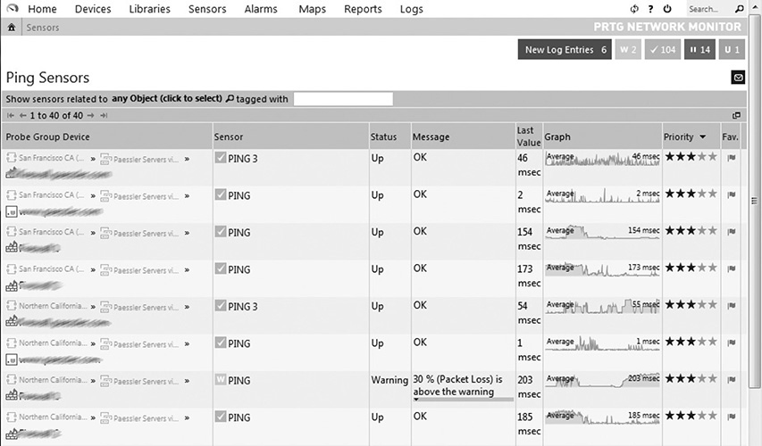
Figure 12-9 PRTG network monitor

Shared vs. Dedicated

A shared network is one that is utilized for multiple purposes, resulting in some level of contention for resources. Dedicated networks are used only for a specific system, application, or site, such as a backup network that is used only for transmitting backup information from production servers to archival servers.

When more than one device requests the service and resources of a network, it is termed shared bandwidth. When only one sender and receiver pair is capable of unrestricted communication in a network, it is termed dedicated bandwidth. Even though dedicated network communication comes with the advantages of flexibility and reliability in terms of bandwidth utilization, this boost in performance comes at a higher cost because a unique network must be put in place and managed for each system or application rather than all systems and applications utilizing a single network.

Teaming

Teaming is a form of link aggregation and failover used in network interfaces to combine multiple connections, increasing the throughput of the network when compared to a single connection. This also helps in improving the reliability of the network since multiple connections provide redundancy of data. Link aggregation can be performed at all three lower levels of the OSI Model. The primary advantages of link aggregation are that it addresses problems such as bandwidth limitations and lack of resilience.

Class of Service

The Ethernet class of service (CoS) was introduced in Chapter 3. CoS is a way of prioritizing types of traffic at layer 2 using one of eight CoS levels, referenced as CS0 through CS7, with CS0 offering the lowest priority and CS7 the highest. CoS can have a tremendous impact on bandwidth. Overall, this impact should be good because priority will be given to the traffic that is deemed most critical. Users of lower-priority applications, however, may complain of bandwidth problems when a significant quantity of high-priority traffic exists on the network such as Voice over IP (VoIP) or video conferencing.

Adequate Share Capacity

It is important to understand the expected utilization and performance requirements for shares so that they can be provisioned appropriately. Shares with high-performance requirements or high load might need to be on a separate set of disks, whereas multiple low-performance shares or those that are infrequently used could reside on the same set of disks. Growth is also a concern for share placement.

Performance Metrics and Tools

There are many tools available, both online and as stand-alone third-party applications, to assist network administrators in their task of analyzing the performance of a storage device or network. Most storage vendors make software to manage performance on their devices, such as the Hitachi Tuning Manager, EMC ControlCenter, NetApp SANscreen, IBM Tivoli Storage Productivity Center, Dell EqualLogic SAN Headquarters, HP Storage Essentials, and Brocade Data Center Fabric Manager. However, you should know that these tools are not often bundled with the hardware, so they must be purchased separately. Some third-party tools include Solarwinds Storage Resource Monitor. This tool works for EMC CLARiiON, Dell modular disk, IBM DS3000 through the DS55000, and Sun StorageTek 2000 and 6000 models. There is also a free product called Solarwinds SAN Monitor that offers some storage performance and capacity information.

This is not an easy task since there are many performance metrics that must be considered to calculate the exact values that would result in network or system optimization. Monitoring performance enables organizations to identify issues as and when they occur, thereby preventing major failures and faults. The performance metrics tools for networking should track the response time and availability of networking devices along with uptime and downtime of routers and switches. The tools that are employed for analysis of performance have many built-in dashboards and reports that help support staff.

Before purchasing and installing any tool, it is necessary to thoroughly understand the minimum and recommended system requirements for the application to run efficiently and as expected. A system’s random access memory (RAM), available hard disk space, network connectivity, operating system (OS), and central processing unit (CPU) speed will need to be known in order to determine whether the performance analysis tool is compatible with your system. It is never a good idea to barely meet the minimum requirements. These requirements will allow the program to run, but it will not be a very pleasant experience because the program will perform quite slowly for you and other users of the system.

It is best to exceed the recommended specifications when deploying an application. This is partially to help plan for future upgrades. No application is free from patches and updates as new vulnerabilities and bugs are discovered, and you will want to allow for the system to be upgraded and patched without requiring a hardware upgrade first.

Switch

Both iSCSI and FC use a device called a switch, and the two devices are both similar and different. FC switches allow for the creation of a Fibre Channel network that is an important part of a storage area network. Fibre Channel devices allow communication among multiple devices. It also restricts unwanted traffic among various network nodes.

Port Statistics

Port statistics can provide valuable data on the performance of switch ports on the storage network. They can also be used to baseline the performance of the network. Statistics can be viewed on the switch management interface, or they can be collected using Simple Network Management Protocol (SNMP) or Storage Management Initiative-Specification (SMI-S) by a storage management tool.

SNMP is a method for devices to share information with a management station through UDP ports 161 and 162. SNMP-managed devices allow management systems to query them for information. Management systems are configured with management information bases (MIBs) for the devices they will interact with. These MIBs define which variables can be queried on a device. Download the MIB for your switch model and load it into your management tool. Next, configure the switches and your management tool with the same community string and point the switches to your management tool as the collection point so that the tool will receive the SNMP messages.

SMI-S is a protocol used for sharing management information on storage devices. It is a good alternative to SNMP for managing devices such as storage arrays, switch tape drives, HBAs, converged network adapters (CNAs), and directors. It is a client-server model where the client is the management station requesting information and the server is the device offering the information. The Manage Engine OpStor tool, shown in Figure 12-10, shows several fabric switches and how many ports are used, operational, and problematic.

---

Figure 12-10 Manage Engine OpStor

Some important port statistics include the frame check sequence, total input drops, total output drops, and runt counters.

•   Input queue This is the number of frames currently waiting in the input queue. While a switch may have many ports, it is not actually capable of sending and receiving data on every port simultaneously. When many frames are received at the same time, some are put into an input queue and held there until the switch can send them to their destination port. If the queue fills up, the oldest frames are dropped, and new ones are added. Each dropped frame increases the total input drop counter.

•   Output queue Similar to the input queue, the output queue holds frames that are waiting to be sent down a destination line. Many devices may desire to send data to the same device, but it can receive only so much data at once, so some data must be queued. If the queue fills up, the oldest frames are dropped, and new ones are added. Each dropped frame increases the total output drop counter.

•   Runt counters Runts are frames that are smaller than 64 bytes, the minimum Ethernet frame size.

•   Frame check sequence (FCS) FCS is a field in frames that is used to detect errors. FCS accomplishes this through cyclic redundancy checks (CRC) or parity. CRC generates a number using a mathematical formula from the data in the frame. If a different computation is achieved on the receiving end, the frame is considered corrupt. Parity assesses all the bits in the frame and includes a 1 if the bits are odd and a 0 if they are even.

Thresholds

Thresholds allow limits to be set for an interface, switch, or globally. These then allow the network traffic to proceed efficiently. These can still be overridden as necessary but only at the switch or interface level. Effective performance can use thresholds to determine when additional links should be added or when traffic prioritization must be put in place.

Hops

Each OSI layer 3 and higher device along the way from the source to destination is known as a hop. Layer 3 and higher devices include routers, firewalls, proxies, and layer 3 switches, and they can also be known as gateways since they are the point at which packets enter or leave a network segment. The hop count is a component of end-to-end latency. Each hop requires processing of the packet or frame, and that adds a delay. This is one reason why some routing protocols use hop count as their primary or only metric in determining route cost. Each packet is given a time to live (TTL) that defines how many hops it can traverse before the packet is dropped. Each hop decreases the TTL by one before sending the packet to the next hop. The device that drops a packet will send back an Internet Control Message Protocol (ICMP) time exceeded message to the sender notifying them of the dropped packet.

The tracert command can be used to view each of the hops between a source and destination. The command shows the latency for each hop so you can see where problems might lie in the network or internetwork. Figure 12-11 shows the tracert command executed for www.snia.org.

---

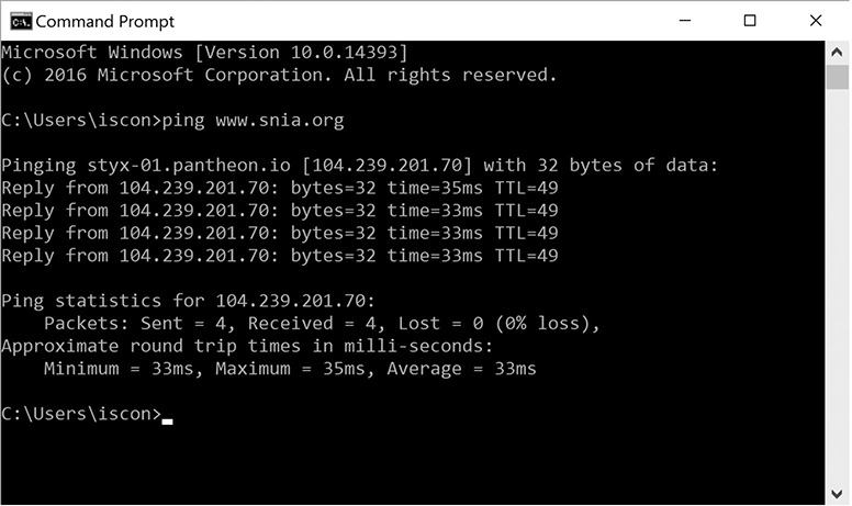
Figure 12-11 Tracert command

Port Groups

Port groups connect more than one port together under the same configuration, thereby providing a strong base for virtual networks that are connected together. The port groups have a unique network label based on the current host. The port groups that are connected together to the same network are always given with the same network label. Moreover, port groups that are connected with more than one network have more than one network name.

ISL

In an FC switched-fabric (FC-SW) network, storage devices and hosts are connected to one another using switches. Switches are devices with many ports that allow connectivity between devices. FC-SW fabrics scale out by adding switches connected together using interswitch links (ISLs). The ports comprising the ISL need to be FC E-ports (see Chapter 3), a specific port designed for communication between FC switches.

The ISL port statistics maintain information related to Ethernet frames or errors that traverse ISLs. ISL port statistics can be viewed on the switch interface or through management tools that collect SMI-S information from the switch.

ISLs may need to be expanded if traffic data is being dropped and queues are full. Expanding an ISL means adding one or more ports to the ISL, which increases the available bandwidth. Another option is to move connections from a saturated switch to another switch that is less saturated.

Communication crossing the ISL will contend for available bandwidth, so ISLs can be a primary limiting factor in FC SAN performance. You can achieve the best performance by reducing the number of ISLs that need to be crossed.

Bandwidth

Bandwidth is a term that is used for measuring data communication over a network. It is usually expressed in the form of bits per second, and the other forms of expression are kilobits per second, megabits per second, gigabits per second, and so on. Bandwidth also refers to the maximum capacity of a networking channel. This is especially important for WAN connections. Track bandwidth metrics and consider upgrading bandwidth speeds or reducing network traffic if utilization approaches the maximum provided by your Internet service provider (ISP).

Packet capture and protocol analysis tools can also be helpful in diagnosing network or bandwidth issues. Wireshark and Capsa are tools that will collect all the packets that traverse a port. This data can be analyzed to determine what type of data was flowing through the connection, which nodes were part of the communication, and the protocols and ports utilized. Statistics can be computed based on the data such as percentage of data per protocol, most used protocols, most popular nodes, and so forth. These can be helpful in diagnosing issues or in creating benchmarks.

Array

The storage array is a device that functions as a data storage machine with high availability, ease of maintenance, and high reliability. Storage arrays typically come with an interface that allows storage administrators to view performance metrics such as cache hits, CPU load, and throughput. These items are discussed in more detail next.

Cache Hit Rate

When a request is made for data that exists in the cache, it is known as a cache read hit. The storage array can immediately service the request by sending the data over its interface without retrieving the data from disk. Cache read hits result in the fastest response time. Use the cache hit ratio to optimize cache sizes.

CPU Load

The CPU load is a measure of the amount of work the CPU is doing as the computer functions. Tools such as the Windows Activity Monitor or Task Monitor can show processor or CPU utilization as a percentage of capacity on the host, and array tools can show similar statistics for storage arrays. High CPU load could indicate the need for a faster processor or throttling of certain storage services. This can help to identify applications that may need to be throttled or uninstalled to improve processor availability. Figure 12-12 shows performance statistics for an EMC storage array, including the CPU utilization for the data mover. This screen was obtained through the system management software provided by the storage vendor.

---

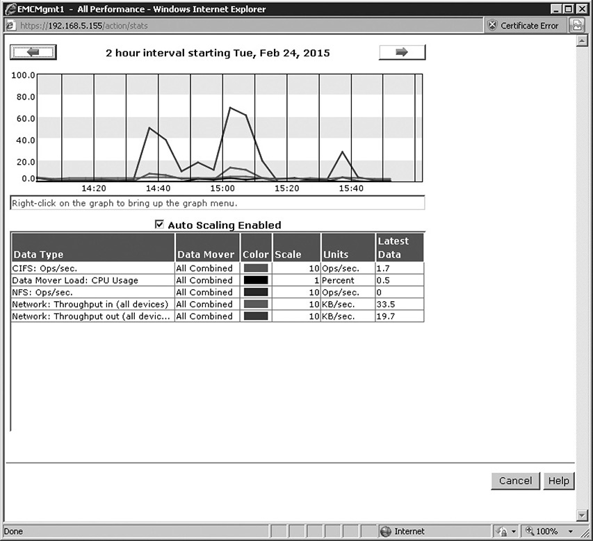
Figure 12-12 Storage management performance

Port Stats

The port stats on the array are similar to those on a switch. The following are some useful statistics:

•   Frame check sequence (FCS) FCS is a field in frames that is used to detect errors. FCS accomplishes this through CRC or parity. CRC generates a number using a mathematical formula from the data in the frame. If a different computation is achieved on the receiving end, the frame is considered corrupt. Parity assesses all the bits in the frame and includes a 1 if the bits are odd and a 0 if they are even.

•   Output queue The output queue holds frames that are waiting to be sent down a destination line. If the queue fills up, the oldest frames are dropped, and new ones are added. Each dropped frame increases the total output drop counter.

•   Runt counters Runts are frames that are smaller than 64 bytes, the minimum Ethernet frame size.

Bandwidth

Front-end ports are used for host connectivity. Hosts will directly connect to these ports or, more commonly, connect through a SAN via a switch. The front-end ports need to be configured to work with the transport protocol that is in use on the network, such as Fibre Channel (FC), Internet Small Computer System Interface (iSCSI), or Fibre Channel over Ethernet (FCoE). Back-end ports are used to connect a storage array controller to storage shelves containing disks. Back-end connections will use whichever technology is specified by the array such as FC or SAS.

Thresholds

Thresholds were discussed earlier for switches. Thresholds on storage arrays are often defined for available capacity. The Manage Engine OpStor tool, shown in Figure 12-13, shows several storage arrays, their capacity, how much is used, and how much is available (free).

---

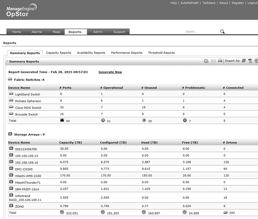
Figure 12-13 Manage Engine OpStor array capacity thresholds

Throughput

Throughput is the amount of data transferred over a medium in a measurable time interval, and it is usually measured in IOPS, mentioned at the beginning of this chapter.

Front-end ports are used for host connectivity. Hosts will directly connect to these ports or, more commonly, connect through a SAN via a switch. The front-end ports need to be configured to work with the transport protocol that is in use on the network such as Fibre Channel, Internet Small Computer System Interface, or Fibre Channel over Ethernet. Front-end port throughput determines how much data can be transferred to and from the storage array to the devices accessing it. Ensure that the front-end ports can provide enough throughput for both normal and peak loads.

Back-end ports are used by the controller to communicate with disk shelves and other array components such as virtualized arrays. Back-end connections use whichever technology is specified by the array such as FC or SAS. Throughput for back-end ports determines how much data can be transferred from the disks in a storage array to the storage array controller. This is one component for determining how long it will take the array to process requests.

I/O Latency

Latency is the time it takes to go from source to destination. In other words, it is the travel time. Latency is a factor in communications that occur within storage arrays or even storage components, and it is also a factor in network communications. Electrical impulses and light have a maximum speed, so longer distances will result in higher latency. Of course, sending data from one place to another is not as simple as dropping it on a wire. Devices forward or route the data to its destination along the way, and each of these devices will add latency to the equation. Latency measurements are typically described in milliseconds.

Host Tools

The following are some of the popular tools that can come in handy for analyzing the state and performance of the system.

Sysmon

Sysmon is a Microsoft Windows tool developed by Mark Russinovich and Thomas Garnier. The tool is installed as a driver and logs additional activity to the event log about network connections, running processes, and file changes.

1.   Download sysmon from http://download.sysinternals.com/files/Sysmon.zip.

2.   Extract the sysmon.exe file from the sysmon.zip file to your computer.

3.   Open a command prompt and navigate to the directory where you copied sysmon.exe.

4.   Install the sysmon service and driver by executing the following command:

sysmon –accepteula –i

You have now installed the driver and configured the service with default settings, as shown in Figure 12-14. The sysmon service will now log events and place them in the Windows event log. The service will start automatically whenever the system restarts, so you will not need to execute these steps again unless the service is disabled. To uninstall the driver, execute the following statement:

---

Figure 12-14 Sysmon default settings

sysmon -u

Performance Monitor (perfmon)

Performance Monitor (perfmon) is a Windows tool that gathers performance metrics, called counters, and displays them in a graph format. This is how you use the tool:

1.   Go to Start | Run and then type perfmon and press enter.

2.   The Performance Monitor tool will load.

3.   Click Performance Monitor on the left side of the screen under Monitoring Tools, and a graph will appear. The default counter, Processor Time, is displayed in the graph.

4.   Click the green plus sign to add more counters. Figure 12-15 shows the Bytes Sent/sec counter being added for the Broadcom NetXtreme Gigabit Ethernet adapter. Select the counter you want and then click Add. Click OK when done adding counters.

---

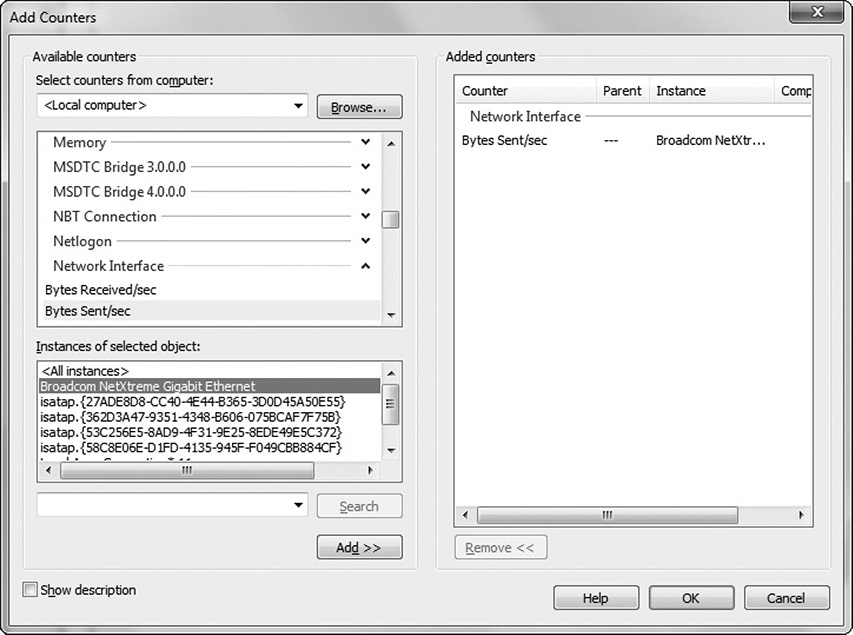
Figure 12-15 Adding counters to Performance Monitor

The counters will appear in the graph. You can hide the Processor Time counter by unchecking the box next to it. Figure 12-16 shows the Performance Monitor graph for Processor Time and the Bytes Sent/sec counter added in step 4.

---

Figure 12-16 Performance Monitor graphs

IOstat

IOstat is a Linux tool that provides users with reports on performance statistics. At the Linux shell or terminal, type iostat, and you will be presented with the default counters of CPU usage and disk reads and writes for each logical volume. You can view network statistics by typing iostat –n. IOstat can also be scheduled to run at intervals and can log on to files for later review. Figure 12-17 shows the output for IOstat with the default counters.

---

Figure 12-17 IOstat with default counters

Network Troubleshooting

Troubleshooting network problems involves several steps. First the source or location of the problem must be pinpointed. At this stage, all affected resources such as nodes, devices, or paths are identified. Next the nature and extent of the problems must be determined. This may involve a range of resources, such as conducting sophisticated network analyses and reviewing user accounts of the problems. Once the scope and nature of the fault have been determined, in-house knowledge bases that document previous system malfunctions may provide a quick path to resolution. The creation of and maintenance of such knowledge bases have proven invaluable in reducing mean time to repair (MTTR).

Experience has taught network administrators that many system faults are attributable to simple triggers or conditions. The following discussion provides practical advice in approaching level 1 problem resolution.

Changes, both authorized and unauthorized, are often the biggest culprits. Mistakes can be made in changing the configuration, naming conventions, or associations. Users are typically unaware of or outright dishonest as to the changes they’ve made or the potential for error associated with them. Ask simple questions to get at the root of problems. Did the user change their password? Have they installed any software since the last time they performed the action that currently does not work? Have they enabled or disabled system services, removed files, or changed system settings? If the change sounds like a plausible explanation for the problem, reverse the change and test again.

Simple tests can be another first line of defense in using simple practical means of problem resolution. For example, if a user cannot connect to a NAS, you might begin by pinging the NAS by name. If the NAS pings by name, the device is up and available, the name to IP address mapping provided by DNS or a host file is correct, and the computer you are running the ping command from has a connection to the NAS.

Determine whether a nearby computer attached to the same resource is experiencing the same problems. If both have the same issue, you may try it again from a machine on another virtual LAN (VLAN) or from a host on the same VLAN as the NAS. This could eliminate network segments. If the NAS does not ping, you may check to see whether it is powered on or in a startup error state.

Continue narrowing down the scope until you have a few possible solutions to test. Test each possible solution until you find one that works. If none of the solutions works, reevaluate your scope and assumptions to come up with new possible solutions. Once the solution is found, document it and verify that the problem has been resolved. Review whether changes should be implemented so that this problem can be avoided in the future.

Connectivity Issues

Connectivity issues are problems that inhibit or prevent a device from communicating on a network. Indicators include such things as services failing because they cannot connect to storage resources, users complaining that data is inaccessible or shares are unavailable, errors on failed redundant paths, or excessive errors in communication hardware. Troubleshooting these issues requires the storage administrator to identify the component, such as a cable, Gigabit Interface Converter (GBIC), or HBA, that is causing the problem.

Begin the troubleshooting process by isolating and eliminating options until you are left with the culprit. In the case of a bad connector, you would eliminate options such as the cable, GBIC, or HBA by trying different cables, GBICs, or HBAs. If the problem remains, you can most likely eliminate the component you swapped out.

Failed Cable

If a host cannot connect to the network but other hosts on the same switch can connect, it could be a problem with the cable, switch port, or network interface card. If you determine that the problem is with the cable, try the following steps:

1.   Make sure the cable is fully seated in the NIC or HBA port and the switch port. You should see status indicators near the cable on the NIC or HBA to indicate whether it is sending and receiving traffic. If you do not see the indicators, unplug the cable and plug it in again.

2.   If this does not work, try replacing the cable with one that you know is good or test the cable with a cable tester to determine whether it is faulty.

Misconfigured Fibre Channel Cable

A misconfigured Fibre Channel cable could cause a loss of connectivity. Open the HBA card properties and check to see what the World Wide Name (WWN) is for the card. Ensure that a zone has been created for the WWN. If so, open Disk Management and rescan the disks to see whether the Fibre Channel disks show up. If multipathing or management software is loaded on the machine, open it and look for card errors. Research errors on the manufacturer’s web site or support pages.

Failed GBIC or SFP

A failed GBIC or small form-factor pluggable (SFP) will have many of the same symptoms of a failed cable. The good news is that a GBIC or SFP is quite easy to swap out. If you have trouble with a fiber cable, try changing this first using the following steps:

1.   Press the release tab on the fiber cable and gently pull it out of the SFP or GBIC. Place plastic safety caps on the fiber cable ends to protect them from damage.

2.   Press the release tab on the SFP or GBIC and pull it out of the switch port.

3.   Insert a new SFP or GBIC of the same type in the empty switch port.

4.   Remove the plastic safety caps and plug the fiber cable into the SFP or GBIC.

5.   If this does not work and this is a new GBIC or SFP installation, verify hardware and software support for this type of GBIC or SFP.

Failed HBA or NIC

If you are unable to establish a connection and replacing the cable does not work, it could be a problem with the HBA or NIC. To replace the card, use the following steps:

1.   Shut down the device and unplug the power cable.

2.   Unplug the cable or cables attached to the failed HBA or NIC.

3.   Attach an antistatic wrist strap to your wrist and secure the grounding click on the wrist strap to a ground.

4.   Open the case and remove the screws around the NIC or HBA.

5.   Pull upward firmly on the card and place it in an antistatic bag.

6.   Insert the replacement card into the slot from which you removed the bad card.

7.   Screw in the card and assemble the case again.

8.   Plug the cables into the new HBA or NIC.

9.   Attach the power cable and power up the device.

10.   Configure the NIC with the IP address the previous NIC had. If replacing an HBA, change the WWN on the zone to the new WWN of the replacement HBA.

Intermittent HBA Connectivity

Intermittent HBA connectivity could be due to latency, saturation of a link, or port errors. Log in to the switch the device is connected to and check for port errors. See whether other devices are having the same problem. If so, check the ISLs between source and destination switches to see whether they are saturated or experiencing errors.

VLAN Issues

A VLAN allows storage administrators to configure a network switch into multiple logical network address spaces, which segments traffic and adds flexibility in network design. The downside is that it can be easy to plug a cable into the wrong port and get a different VLAN, so it is important to document the ports that are assigned to VLANs, the VLAN numbers, and their purposes.

Devices on the wrong VLAN may not be able to connect to certain network resources. Use the ping command to test connectivity to other devices. For example, ping 192.168.3.25 would test connectivity to the host with the IP address 192.168.3.25. A router or a layer 3 switch is required to route traffic between VLANs. If VLAN routing has been set up and VLANs cannot talk to one another, check the cables that connect the VLANs to the layer 3 switch or router and verify that the routing configuration is correct.

If the device is using Dynamic Host Configuration Protocol (DHCP) to receive an IP address, see which network the IP address is on. For example, a network could be divided into three VLANs: 192.168.1.1, 192.168.2.1, and 192.168.3.1. If the device is plugged into the wrong VLAN and it is using DHCP, it may receive an IP address for that VLAN, and this will allow you to determine which VLAN it is on. Check documentation for the port it is plugged into and verify that it is configured for the correct VLAN.

The ipconfig command in Windows and the ifconfig command in Linux display the IP address for a device that can be used to determine which VLAN it is on. The output from the ipconfig command, showing the IPv4 and IPv6 addresses, domain name, subnet mask, and default gateway, is displayed here:

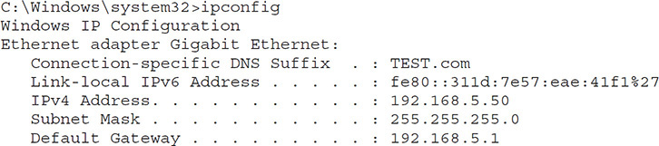
Zoning Issues

Zones are a wonderful way to implement security on a SAN, but they do increase complexity, requiring the storage manager to troubleshoot and manage zones. Chapter 8 describes storage zoning, so we will only briefly review the topic here. Please look back to that chapter if you need additional information. Zoning is a way of defining which devices can access storage resources. Port zoning assigns storage resources to ports on switches. Devices that are connected to those ports can view the storage resources. WWN zoning assigns resources to the unique name assigned to a Fibre Channel HBA. With WWN zoning, a device can be moved to a different port and still access the same resources, but if the HBA is changed, the zoning configuration will need to be updated.

Zoning Misconfiguration

Drives that have been assigned will not show up if zoning has been misconfigured. Hosts on a zoned SAN are provided access to drives, represented on a SAN using their logical unit number (LUN), by mapping that LUN to the host’s WWN. The first step to diagnose this is to check the WWN of the HBA that is in the device. Next, look at the zoning configuration to see which LUNs are mapped to the WWN. Add or remove LUNs from the zone if the correct LUNs do not appear. If the WWN of the HBA is not in the zone, add it.

You may need to issue a rescan after the zoning configuration has been fixed so that the host will pick up the new LUNs. You can issue this command in Microsoft Windows within the Server Manager console with the following procedure:

1.   Open Server Manager by clicking Start; then right-click Computer and select Manage.

2.   Expand the storage container and select Disk Management.

3.   Right-click Disk Management and select Rescan Disks.

4.   (Optional) You may also need to right-click Logical Volumes and place them online once they reappear in Disk Management.

Zoning Errors

Zoning errors can provide valuable insight when troubleshooting a problem. Look for zoning errors in storage array, switch, and HBA error logs because these will provide the most technical information.

Interoperability Issues

There are many components in a storage network that have to operate together. Sometimes the configuration of different devices can come into conflict, reducing performance or losing the connection entirely. One situation that can happen is when a device is connected to a port that is offline. Verify that the port status is set to online on the switch.

Another is duplex mismatch. Check for duplex mismatch by verifying that the duplex setting and speed are set to the same values on the NIC and switch. Duplex mismatch occurs when a switch or NIC is configured for full duplex, while its partner switch or NIC is configured for half duplex. Full-duplex communication allows for data to be sent and received at the same time, while half-duplex communication sends data and then receives data but not both at the same time. Connections can drop, and communication is typically very slow when duplex mismatches occur.

Host Troubleshooting

The following section includes troubleshooting tips for diagnosing host issues. The tips include hardware or software incompatibility, outdated firmware or drivers, incorrect NIC configuration, a bad NIC, storage tiers, improperly connected NIC, incorrect firewall settings, and incorrect cluster or multipath settings.

Hardware or Software Incompatibility

Modern operating systems support a wide range of hardware, but not all hardware is supported by all operating systems. Most operating systems maintain a hardware compatibility list that can be queried to determine whether the device is supported. Another way is to go to the web site for the vendor that produced the hardware component to see whether it has support. Support is usually offered through a piece of software known as a driver that allows the operating system to communicate with the hardware. Search for drivers for the operating system in use.

Sometimes drivers can have compatibility errors. If using Microsoft Windows, check Device Manager for errors. If conflicts exist or the network adapter is being detected as an “other device,” try using the update driver function to have Windows scan for updated drivers automatically. If this does not work, check the vendor’s web site and download the latest driver for your operating system and install it. If this does not work, try uninstalling the driver software and then restart the computer to have Windows redetect and install the device.

Outdated Firmware or Drivers

Modern Linux, Mac, and Windows operating systems will attempt to update drivers automatically with software, but some drivers may not be registered with the operating system vendor and must be updated manually. Check the vendor’s web site and download the latest driver for your operating system and install it.

Incorrect NIC Configuration

Incorrect NIC configuration can limit or inhibit network connectivity. The first step in diagnosing an incorrect NIC configuration is to determine what the current configuration is. The ipconfig (Windows) or ifconfig (Linux) command will display the current configuration of your network cards. Figure 12-18 shows the output of the ifconfig command. From a command prompt, examine the results and then compare them to the documented configuration for the device. If documentation does not exist, determine the default gateway, Domain Name System (DNS) server, subnet mask, and an available IP address. Open the NIC configuration and configure these values; then issue a ping to verify connectivity with the default gateway and other network resources.

---

Figure 12-18 ifconfig

Bad Connector

Begin the troubleshooting process for a bad connector by isolating and eliminating options until you are left with the culprit. In the case of a bad connector, you would eliminate options such as the NIC cable or port by trying different cables, ports, and NICs. If the problem remains, you can most likely eliminate the component you swapped out. Try the connector with a different component that you know is good. If that system is unreachable, try replacing the connector on the device you are having trouble with. If spare components are available, you can try using them in the unreachable system. However, you must first make sure that the component from storage is good before performing this test. Otherwise, you may swap a bad component for another bad component.

Bad Cable

Cable failure is more common than you would think. Both optical and twisted-pair cables are sensitive in their own ways. Optical cables are expensive and sensitive pieces of equipment. If a fiber-optic cable is bent too far, the light inside the cable will be reflected and dispersed, resulting in a loss of signal until the bend is corrected. The fiber-optic core can also be damaged if bent too far and will need to be replaced.

Twisted-pair cabling must not be stretched or the twists will elongate and make it more susceptible to crosstalk (XT). Higher categories have more twists per inch and are more sensitive to stretching than lower-category cables. This is why you can tug on a phone cable quite a bit before losing connectivity, whereas a CAT6 cable might begin to lose data after a few good pulls. Also, don’t run Ethernet cables near power lines or light fixtures because these generate electromagnetic interference (EMI) that can disrupt communications. If cables must be located near power or lights, consider using shielded tubes or tape to provide extra protection against EMI. The bend radius for twisted-pair cabling must be at least four times the outer diameter of the cable to avoid kinking.

You may also run into problems if a cable is longer than its maximum transmission length. The maximum length of optical fiber depends on the data rate, with higher data rates reducing the maximum transmission length since higher data rates suffer greater from attenuation.

The process for troubleshooting a bad cable is similar to that of troubleshooting a bad connector. Swap the cable out for one that you know is good. This may be one from another system or a spare component in storage.

Bad Port

As you can probably guess by now, you can identify a bad port by connecting the system’s cable and connector to a different port. The difference here is that two ports are required to make a connection, so you will have to test both to see whether one or the other is the failed component. If the connection is an ISL, you will need to configure another ISL on a new port on one switch and then move the cable to that port. If the connection still fails, move the cable back to the initial port, remove the configuration you just added, and add a configuration for an ISL on a different port on the second switch in the ISL connection.

If the connection is between a switch and an end device such as a host, array, or tape drive, try connecting to another port on the host, array, or tape drive to see whether the connection works. In some cases, you will not have another port to connect to on the device because all ports may be in use. In this case, your troubleshooting options will depend on how the device is configured. If all the ports are configured as one link, you can swap the cables on the device and use the device management software to view the link status. If the good port goes offline and the one that previously was offline goes online, you have identified the culprit. Ensure that you follow your organizational change management and notification procedures before making changes to production hardware, even when troubleshooting an issue.

You can use the fcping command to issue an FC Extended Link Service (ELS) request to a port or pair of ports by using their WWN. Ports that receive an ELS request will respond, letting the user know that it is active and able to communicate.

Running the fcping command from an FC switch to WWN 21:01:00:E0:8B:A5:26:6A would produce the following output:

The first line after the command confirms that you are pinging WWN 21:01:00:E0:8B:A5:26:6A, which has an FC-ID of fd1091. Each ELS reply is then given, along with the time it took to receive a reply. The last line of the output shows the statistics beginning with the shortest (min), average (avg), and longest (max) ELS reply in the set. The output of this command shows that all five out of five pings were sent and ELS replies were received for each of the five, with the shortest response taking 902 microseconds, the average 1070, and the longest 1222.

Bad NIC

If you are unable to establish a connection and replacing the cable does not work, it could be a problem with the NIC. To replace the card, use the following steps:

1.   Shut down the device and unplug the power cable.

2.   Unplug the cable or cables attached to the failed NIC.

3.   Attach an antistatic wrist strap to your wrist and secure the grounding click on the wrist strap to a ground.

4.   Open the case and remove the screws around the NIC.

5.   Pull upward firmly on the card and place it in an antistatic bag.

6.   Insert the replacement card into the slot from which you removed the bad card.

7.   Screw in the card and assemble the case again.

8.   Plug the cables into the new NIC.

9.   Attach the power cable and power up the device.

10.   Configure the NIC with the IP address the previous NIC had.

NIC Improperly Connected

The main cause of improperly connected NICs is that they are not fully seated. To verify that the NIC is seated, use the following steps:

1.   Shut down the device and unplug the power cable.

2.   Unplug the cable or cables attached to the NIC.

3.   Attach an antistatic wrist strap to your wrist and secure the grounding click on the wrist strap to a ground.

4.   Open the case and push down on the NIC to ensure that it is fully seated. Look at the connection between the card and the device motherboard and ensure that it is flat against the interface port.

5.   Tighten the screw down on the NIC card so that it cannot wiggle in the case.

6.   Plug the cables into the NIC again.

7.   Attach the power cable and power up the device.

Incorrect Firewall Settings

Firewall software is used to block communications over specific logical ports such as port 443 for Secure Sockets Layer (SSL), port 22 for Secure Shell (SSH), port 23 for Telnet, port 389 for Lightweight Directory Access Protocol (LDAP), or 161 for Simple Network Message Protocol (SNMP). Connections may be blocked to and from the device if a firewall rule has not been configured for the connection. If you suspect the firewall may be blocking the connection, temporarily turn the firewall off and see whether the connection resumes. If the connection works, run the following command to see which port the connection is utilizing:

netstat –a

The netstat command will list many connections, as shown in Figure 12-19, so you will need to know the IP address of the computer connecting to it so that you can identify the line that contains the connection in netstat. Next, turn the firewall back on and create a rule in the firewall for the connection specifying the port identified in netstat.

---

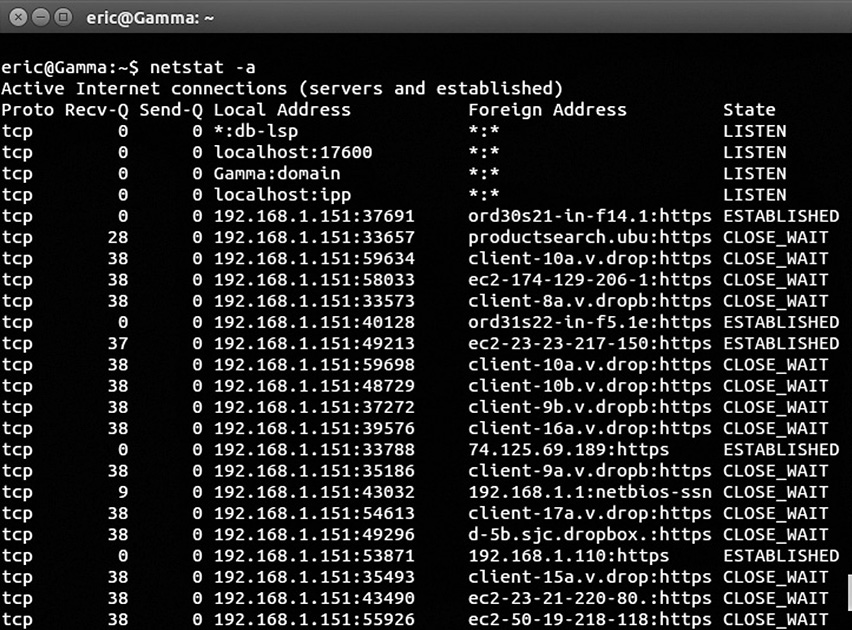
Figure 12-19 netstat -a command

Incorrect Cluster or Multipath Settings

Cluster settings allow multiple computers to connect to the same resources, but if incorrectly configured, multiple computers could try to modify data at the same time, resulting in conflicts. Clusters usually have a software component that is built into the operating system. Ensure that the clustering component is enabled and that all the nodes appear in the cluster.

You might also find that only one node can access the LUNs. If this is the case, ensure that the storage device LUN mapping is set for cluster and that the WWNs for each node in the cluster are in the LUN mapping.

Multipathing allows multiple NIC or HBA ports to be used for load balancing and failover. This is accomplished through built-in operating system multipath I/O (MPIO) drivers or via vendor software such as Hitachi Dynamic Link Manager (HDML) or EMC PowerPath. Open the software and verify that all NIC or HBA ports are configured in the multipath and that load balancing and failover are enabled. Also, check for errors in the software and research errors on the vendor’s web site if errors are found.

Backup Troubleshooting

Reliable backups are crucial in maintaining adequate system availability and preserving organizational documents and other intellectual property. Backup systems need to be regularly monitored for backup failures, errors, and warnings. Storage or backup operators often create alerts for these events so that they can correct issues as quickly as possible. In some cases, backup alerting may be integrated with other IT service processes such as an issue tracking system, also known as a trouble ticket system or request management system. Such systems have a workflow defined to create a task based on a system event. The task is then assigned to a person or placed in a queue. That person will then need to resolve the error. Some of the most common backup problems are described here. They include space limitations, open files, blocking by virus scanners, and incorrect permissions.

Space Limitations

It is important to properly size backup drives to avoid space errors and to ensure that the required files are archived successfully. Proper planning requires understanding the current size of backups and growth rates, because backups need to be able to handle current demand and short-term or long-term backup growth. Most backup suites will perform compression on the backup files as they are stored, and many will deduplicate the data. Both methods can dramatically reduce the amount of space required to store data, but they can also make it difficult to understand how much space will actually be consumed by initial and successive backup jobs. Some backup vendors offer estimating tools to help with this process. You can also perform your own computations.

Let’s say you have 4TB of data to back up, with a 5 percent (200GB) change in data for every incremental backup. Now if you do an incremental backup every day, you require 1,400GB (that is, 200GB × 7). Having a full backup once a week will require the entire 4,000GB of space needed weekly. Thus, you would need 5,400GB (or 5.4TB) of free space for the backups. Over the course of a month, you might have four weekly backups and the incremental in between, which is overwritten each week. That would require 4,000GB each week and one week of incremental backups at 1,400GB. Together that is 17,400GB. As you can see, space requirements increase quickly with multiple backup sets.

If there is a 2:1 compression ratio for the data, you would need 8,700GB (17,400GB / 2) of storage space per month for a compressed backup. If the deduplication ratio is 4:1, you would need 5,350GB (17,400GB / 4). If you both compress and deduplicate the data, assuming the ratios stay the same, it would be half the size due to the 2:1 compression ratio, so you would need 2,625GB.

Running Out of Space on the Destination

If you are running out of space on the destination drive, add more capacity, decrease the backup interval, or change the backup method to utilize fewer full backups. It is also common to find old backup files from jobs that have been changed or removed that are still resident on the backup server. If these files are no longer needed, remove them to clean up space.

Running Out of Space on the Target

Backup software will sometimes create temporary files on the target machine when it is backing up files. However, the backup job may fail if insufficient space is available on the target. Microsoft Volume Shadow Copy Service (VSS), for example, requires around 1GB of free space on each volume being backed up. The Microsoft VSS backup error shown here clearly states the problem:

You can troubleshoot out-of-space errors by performing the following steps:

1.   If there are backups older than a certain date, archive them on a separate disk, pending deletion if the organization determines they are not needed.

2.   Run Windows disk cleanup to get rid of old files.

3.   Make sure to empty the Recycle Bin so that the space will be reclaimed by the system.

4.   Remove temporary files.

5.   Empty web browser cache.

6.   Delete unused files in the downloads folder or folders that may have been downloaded by users or applications.

7.   Remove or deduplicate redundant files on the computer.

Open Files

Backup systems must make archival copies of files, but sometimes those files are in use by users or applications. For example, a backup of a file server may be scheduled for 1:00 A.M. but some users might still have documents open on their workstations when they go home for the night, so those documents are currently locked for editing. Virus scans could also leave files open and result in an open file error. In addition, application files are often in use by their associated applications and will require interaction between the application and the backup software in order to back up those files while the application is in use.

For example, database applications may load database files into memory and have exclusive control over those files the entire time the database service is running. It is not practical to shut down the database servers to perform a backup because this would result in the unavailability of the application, so the backup software needs to be able to interact with the database application. Rather than just backing up files, application-specific agents can back up databases or portions of data sets within a file. An e-mail backup could be performed on select mailboxes or just on public folders using the backup agents, whereas a simple file backup would not offer this granularity. Similarly, hypervisors (servers that host virtual machines) have agents that allow for virtual machines or files within virtual machines to be backed up.

Backup systems have various methods to archive files that are open, but those systems must be enabled for the resource in order for them to function. Here are some examples of open file errors:

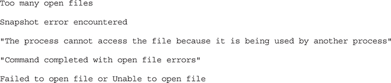
You can troubleshoot open file errors with the following steps:

1.   Install application-specific backup agents. For example, if you’re backing up a database server running Microsoft SQL Server, install the backup agent for Microsoft SQL Server. If you’re backing up an e-mail server, install the e-mail agent. The agents are provided by the backup software vendor, and a separate license is typically required for each agent. Configure the backup job to back up elements of that system rather than the files themselves. For database servers, choose databases or even tables within the database. For e-mail servers, choose the mailboxes, calendars, or folders you want to back up. For hypervisors, choose the virtual machines you want.

2.   Many open-file backup systems for Windows rely on the Microsoft Volume Shadow Copy Service. Ensure that VSS is running on the target machine.

3.   Give the backup agent a user account with sufficient privileges to read the files, or access the application and ensure the account is not denied permission. In some cases, this may require administrative credentials (for example, when backing up critical services such as Microsoft Active Directory or certificate services).

4.   Set users to automatically log off late at night for maintenance. Notify the users that this will happen in case they need to run a program overnight.

Virus Scanning

Virus scanners look for malicious or suspicious activity on a machine and block that activity when they find it. Suspicious activity is determined by virus signatures or patterns of behavior. Backup software can sometimes appear suspicious to antivirus scanners because backup software attempts to read many files and change their archive bit. Backup agents may be terminated by the target’s antivirus software if it believes the backup agent is acting suspiciously.

Backup jobs that are being blocked by virus scanners often run extremely slow and produce a large number of errors, typically one or more for each file that could not be accessed due to blocking from the virus scanner. If you determine that backup failures are the result of antivirus software on the host, use the following procedure to exclude or whitelist the backup agent in your antivirus software. It is a best practice to deploy exclusions and whitelists using a central administration utility so that changes do not have to be made on machines individually. It is also a best practice to test exclusions on several machines before deploying the changes to all machines. Follow this procedure to exclude the backup service from antivirus scans:

1.   Identify the filename and path of the backup agent process.

2.   Open the antivirus utility or central administration utility and navigate to the location where applications can be marked safe. Antivirus vendors may use different names for this section. Some names include application exclusions, whitelisted applications, and safe applications.

3.   Browse to the path where the backup agent process resides and select the backup agent executable to exclude agent activity from virus scans.

Permissions

Backup software needs to have permission to access the files in a backup set on the target machine. When a backup is made, the program needs to have the ability to read the files and directories that are part of the backup set. Here are some examples of permission errors:

The first error you might run into is a lack of permission for the file or folder that is selected on the target server. Correct this error by granting read access for the target directory to the account the backup agent is running under. You can also receive permission errors if the account the backup agent is using is locked out or disabled. Unlock it if it is locked, or enable it if it is disabled. Enabling or unlocking a local account is performed in computer management on the local machine if running a Windows server. Enabling or unlocking a domain account is performed on a domain controller using the Active Directory Users and Computers snap-in in a Windows environment.

Permission errors can occur if the account is denied access. Verify that the target folder does not have a deny permission set for the account that the backup agent uses. Deny permissions always take precedent over allow permissions, so the agent account could be granted access but still be unable to access the files. Remove the deny if it is in place. Sometimes a deny permission is inherited from a parent directory. Disable inheritance on the directory and then remove the deny. This will remove the deny on the folder and subfolders but preserve the deny for higher-level folders. Similar errors can occur if the account is denied the special permission to log on as a batch job. Make sure that the account is not part of the “deny logon as a batch job” policy in the Windows domain controller security policy or in the local policy of the server. Log on to a Windows domain controller and use the Group Policy Management Console to change this for a domain policy, or use “modify the policy on the local machine” if the computer is not part of a domain.

You might receive permission errors if the password for the backup agent account has expired. It usually best to set a very complex password on the backup account and to change the password manually rather than automatically expiring the password or setting it to a change interval, because if the password is not changed within that interval, the backup agent account will not authenticate. Storage administrators will need to ensure that they change the password on each service that uses the account in order to avoid authentication errors. If a password is not updated on each service, some targets may receive permission errors. Verify that the password used by the service account is correct. Retype the password into the service settings and then restart the service. Another administrator may have changed the password but did not update the service settings for each service that uses the account.

Some errors that appear to be permission errors are actually connectivity errors. First verify that you can ping the target. You can ping the target by name, and this will verify that the backup server can correctly resolve the DNS name to an IP address, and it will also confirm whether the machine is responding. If the machine does not respond, check and make sure that it is connected to the network and that it is running. You might also receive a permission error that is actually a connectivity problem if a local server firewall or hardware firewall in between the target and the backup server is blocking the connection. Attempt to telnet to the target machine from the backup server using the port the backup agent uses. If this connection fails, add a firewall rule to allow that port or service through. The following command verifies connectivity between the backup server and a target with the IP address 192.168.10.220, assuming the agent uses port number 6103:

Telnet 192.168.10.220 6103

Chapter Summary

The goal of this chapter was to provide you with a solid foundation in the practices and principles associated with maintaining business continuity through network optimization. The metrics used to measure network performance were presented, and we discussed how their interaction impacts the day-to-day operation of an enterprise. The number of operations or instructions a storage device is able to handle was identified as an important factor at layer 1 of the OSI model—the physical layer.

Timing and scheduling were discussed as means of maintaining a balance between network functionality and monitoring. Defragmentation, or defragging as it is more popularly referred to, is a process by which misaligned files and wasted space on a storage medium are optimized. The sheer capacity of modern-day storage devices makes this a time-consuming and complicated process that could potentially impact peak-time traffic by stalling critical system cycles and resources.

The similarities and differences between standard SATA and other hard drives were contrasted and compared to SSD technology. Each type of disk benefits from different forms of optimization and robustness. The design, architecture, and shelf life of various storage media must be taken into consideration because each will present its own unique opportunities and challenges for the network administrator. The latter part of the chapter went into a more technical discussion of the various types of errors and offers practical steps for identifying, isolating, and ultimately resolving them.

The maintenance of documentation or creation of a knowledge base cannot be overemphasized. This is perhaps the most potent tool in a network administrator’s arsenal. Many administrators focus on sophisticated tools or procedures, failing to reap the benefits that could be derived from documenting the ways in which problems were resolved. This data not only provides a means for rapid MTTR, but also may aid in identifying and tracking patterns that, when integrated into the overall business continuity planning, help maintain a high level of performance while leveraging network investment.

Reliable backups are crucial in maintaining adequate system availability and preserving data integrity. Backup systems need to be regularly monitored for backup failures, errors, and warnings so that they can be resolved in a timely manner. Storage administrators should be familiar with common issues and resolution steps. Some common backup issues discussed here include running out of space on the target or the destination, open files, virus scanning, and permissions.

Software References

Various tools were mentioned in this chapter. For your convenience, a link is provided for each tool here so that you can download or learn more about them. Some tools can be purchased directly, while others require contacting the vendor.

•   Brocade Data Center Fabric Manager
www.brocade.com/downloads/documents/data_sheets/product_data_sheets/DCFM_DS_00.pdf

•   Cacti
www.cacti.net

•   Capsa
www.colasoft.com/capsa/

•   Dell EqualLogic SAN Headquarters
www.dell.com/downloads/global/products/pvaul/en/equallogic-san-headquarters.pdf

•   EMC ControlCenter
www.emc.com/data-center-management/controlcenter.htm

•   EMC Powerpath
www.emc.com/storage/powerpath/powerpath.htm

•   Hitachi Dynamic Link Manager
www.hds.com/products/storage-software/hitachi-dynamic-link-manager-advanced-software.html

•   Hitachi Tuning Manager
www.hds.com/products/storage-software/hitachi-tuning-manager.html

•   HP Storage Essentials
www8.hp.com/us/en/software-solutions/storage-essentials-resource-management/

•   IBM Tivoli Storage Productivity Center
www-03.ibm.com/software/products/en/tivostorprodcent/

•   Manage Engine OpStor
www.manageengine.com/products/opstor/

•   Microsoft Volume Shadow Copy Service (VSS)
https://msdn.microsoft.com/en-us/library/windows/desktop/aa384649(v=vs.85).aspx

•   NetApp SAN screen
www.netapp.com/us/products/management-software/sanscreen/

•   PRTG network monitor
www.paessler.com/prtg/

•   Solarwinds Storage Resource Monitor
www.solarwinds.com/storage-manager.aspx

•   Solarwinds SAN monitor
www.solarwinds.com/products/freetools/san_monitor/

•   Splunk
www.splunk.com

•   Wireshark
https://www.wireshark.org

•   ZenOss
www.zenoss.com

Chapter Review Questions

1.   What is IOPS primarily used for?

A.   To determine which connection should be throttled

B.   To determine the performance of a drive or system

C.   To determine the amount of reserved or protected space needed to operate

D.   The reorganization of a database

2.   An operation in which data is reorganized so that it can be read sequentially to reduce latency and wear and tear on the disks is called what?

A.   Disk damage reduction (DDR)

B.   Defragmentation

C.   Sequential reorganization

D.   Sequential data systemizing

3.   Which of the following best defines a cache read miss?

A.   When the cache crashes

B.   When data from the cache fails to save to the disk

C.   When the data requested does not exist in the cache

D.   When a request for data that exists in the cache fails to initialize

4.   Consider a RAID 5 consisting of four drives. If the bit string in the first stripe is 100, 101, 110, then what value would be written to the fourth drive?

A.   111

B.   101

C.   000

D.   010

5.   In an embedded switch, what causes the increase in reliability and overall performance?

A.   The allocation of a certain task to a separate board

B.   Network connectivity

C.   All functions are performed at the chip level

D.   The use of gold embedded in the circuit board to increase conductivity

6.   What is the CPU load a measure of?

A.   The amount of work necessary from the CPU to run a single program

B.   The amount of work the CPU is doing as the computer functions

C.   The average load that a CPU can handle under regular conditions

D.   The amount of power necessary to run the CPU

7.   After discovering that a host could not connect to the network, Barnabus determined that there was an issue with the cable. What should Barnubus’ next step be?

A.   Replacing the cable with one that he knows is good

B.   Testing the cable with a cable tester to determine whether it is faulty

C.   Ensuring that the cable is properly connected to the NIC or HBA port and the switch

D.   Checking for issues with the switch or the NIC

8.   Tom is a backup administrator for ABC Tools. He configures a daily full backup of a file server, a NAS share, and a database server that all must remain available 24/7. The backup runs at 2:00 A.M. The next morning Tom checks the backup and finds that the backup failed with the following error on each of the database files: “The process cannot access the file because it is being used by another process.” What should Tom do to resolve the error and ensure that the files are backed up?

A.   Modify the backup job to exclude the database files.

B.   Configure a pre-job execution script that stops the database services and a post-job execution script to start the database services.

C.   Install the backup agent for the database software and reconfigure the backup job to back up the databases using the agent.

D.   Connect to the database server as administrator and grant Tom full control of the root directory.

Chapter Review Answers

1.   B is correct. IOPS is defined as the most basic metric used in measuring storage performance.
A, C, and D are incorrect. A is incorrect because throttling determinations would be based on resource contention, not IOPS. C is incorrect because the amount of reserved or protected space would be determined by the applications running on a volume, not IOPS. D is incorrect because reorganization of a database would be based on variables such as query execution time, index lookup time, and other DBMS statistics.

2.   B is correct. Defragmentation reorganizes the data so that it can be read sequentially to reduce latency and wear and tear on disks due to head and platter activity.
A, C, and D are incorrect. A is incorrect because disk damage reduction is not an industry term. DDR in technology refers to a type of RAM. C is incorrect as well because this is not an industry term. It describes what defragmentation does, but the actual term is defragmentation. D is incorrect because it is not an industry term.

3.   C is correct. A read miss is when data is requested of an array but the data does not reside in cache. In such cases, the data must be read from disk and then stored in cache before it is sent to the user or application.
A, B, and D are incorrect. When cache crashes, the cache would be inaccessible. In redundant cache situations, such as those with redundant controllers, read and write requests would be serviced by the other controller, but this would not result in a read miss. B is also incorrect because saving to disk is a process associated with writing data, not reading data. D is incorrect because cache failures, much like cache crashes, trigger a series of events wholly unrelated to cache read misses.

4.   A is correct. The XOR of the first and second drives is 100, and 101 is 001. This combined with the third is 001 and 110, which is 111. Remember, the XOR is 0 when the bits are the same and 1 when the bits are different.
B, C, and D are incorrect. If you came up with 101, 000, or 010, please check your math again. The XOR of the remaining values 100, 101, and 110 equals 111.

5.   C is correct. In an embedded switch, all functions are performed at the chip level, resulting in increased reliability and overall performance.
A, B, and D are incorrect. A is incorrect because allocating a task to a certain separate board could have a variety of effects depending on the task allocated, the ability of the board to perform that task, and the interconnection between the board and the rest of the switch. B is incorrect because network connectivity is essential to switch performance, but it does not necessarily increase performance. D is incorrect because connectors are built to industry standards and a change to one connector would have no impact unless a change was made to the cable that connects to it and the architecture of the cable.

6.   B is correct. The CPU load is essentially the total of all things that the CPU is currently supporting. For example, if a man is carrying a pallet of bricks, the current load he is supporting is the amount of weight he is carrying in that moment.
A, C, and D are incorrect. A is incorrect because the CPU load consists of much more than just one application’s requirements. C is incorrect because average load is different from load. D is incorrect because load is not determined by power. The CPU must be provided the power required in its specifications, no more or less.

7.   C is correct. Before making any changes, Barnabus should ensure that everything is attached correctly.
A, B, and D are incorrect. A is incorrect because replacing the cable takes more time than checking the connection. It is best to try the easiest thing first to save time in troubleshooting. B is incorrect because testing the cable with a cable tester will require disconnecting it and testing steps that take longer to perform than checking the connection. D is also incorrect because Barnabus determined the problem was with the cable, not the switch or NIC.

8.   C is correct. Tom should install the backup agent for the database software on the database server. This will allow the backup software to talk to the database application to back up the databases while they are running, and the backup software will not need to interface with the locked files that are currently preventing the job from completing. Tom then should reconfigure the backup job to use the agent.
A, B, and D are incorrect. A is incorrect because excluding the database files would not back up the database files. B is incorrect because stopping the database services with a script would make the databases and the applications dependent upon them unavailable to users. D is incorrect because enterprise applications should run under a service account, not an individual user or administrator’s account. Also, the files are clearly locked by the database application in this question, and changing the permissions would not correct the locking issue.