
CHAPTER 15
Signal Processing
Over the years, signal processing has become an increasingly important part of audio and music production. It’s the function of a signal processor to change, augment or otherwise modify an audio signal in either the analog or digital domain. This chapter offers some insight into the basics of effects processing and how they can be integrated into a recording or mixdown in ways that sculpt sound using forms that are subtle, lush, extreme or just plain whimsical and wacky.
Of course, the processing power of an effects system can be harnessed in either the hardware or software plug-in domain. Regardless of how you choose to work with sound, the important rule to remember is that there are no rules; however, there are a few general guidelines that can help you get the sound that you want. When using effects, the most important asset you can have is experience and your own sense of artistry. The best way to learn the art of processing, shaping and augmenting sound is through experience—and gaining experience takes time, a willingness to learn and lots of patience.
THE WONDERFUL WORLD OF ANALOG, DIGITAL OR WHATEVER
Signal processing devices and their applied practices come in all sizes, shapes and flavors. These tools and techniques might be analog, digital or even acoustic in nature. The very fact that early analog processors have made a serious comeback (in the form of reissued hardware and software plug-in emulations, as seen in Figure 15.1) points to the importance of embracing past tools and techniques, while combining them with the technological advances of the day to make the best possible production.
The Whatever
Although these aren’t the first thoughts that come to mind, the use of acoustics and ambient mic techniques are often the first line of defense when dealing with the processing of an audio signal. For example, as we saw in Chapter 4, changing a mic or its position might be the better option for changing the character of a pickup over using EQ. Placing a pair of mics out into a room or mixing a guitar amp with a second, distant pickup might fill the ambience of an instrument in a way that a device just might not be able to duplicate. In short, never underestimate the power of your acoustic environment and your ingenuity as an effects tool.
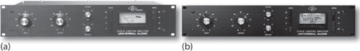
FIGURE 15.1
1176LN limiter: (a) hardware version; (b) powered software plug-in. (Courtesy of Universal Audio, www.uaudio.com. © 2017 Universal Audio, Inc. All rights reserved. Used with permission)
Analog
For those wishing to work in the world of analog (Figure 15.2), an enormous variety of devices can be put to use in a production. Although these generally relate to devices that alter a source’s relative volume levels (e.g., equalization and dynamics), there are also a number of analog devices that can be used to alter effects that are time based. For example, an analog tape machine can be patched so as to make an analog delay or regenerative echo device. Although they’re not commonly used, spring and plate reverb units that can add their own distinctive sound can still be found on the used and sometimes new market.

FIGURE 15.2
Analog hardware in the studio. (Courtesy of Wisseloord Studios, www.wisseloord.nl, acoustics/photo by Jochen Veith, www.jv-acoustics.de)
ANALOG RECALL
Of course, we simply can’t overlook the reason why many seek out analog hardware devices, especially tube hardware—their sound! Many audio professionals are on a continual quest for that warm, smooth sound that’s delivered by tube mics, preamps, amps and even older analog tape machines. It’s part of what makes it all fun.
The downside of all those warm & fuzzy tools rest with its inability to be saved and instantly recalled with a session (particularly a DAW session). If that analog sound is to be part of the recording, then you can use your favorite tube preamp to “print” just the right sound to a track. If the entire session is to be mixed in real-time on an analog console, plugging your favorite analog toys into the channels will also work just fine. If, however, you’re going to be using a DAW with an analog console (or even in the box, under special circumstances) then, you’ll need to do additional documentation in order to manually “recall” the session during the next setup. Of course, you could write the settings into the track notepads, however, another excellent way to save your analog settings is to take a picture of the device’s settings and save it within the song’s session documentation directory.
A number of forward-thinking companies have actually begun to design analog gear that can be digitally controlled, directly from within the DAW’s session. The settings on these devices can then be remotely controlled from the DAW in real-time and then instantly recalled from within the session.
Digital
The world of digital audio, on the other hand, has definitely set signal processing on fire by offering an almost unlimited range of effects that are available to the musician, producer and engineer. One of the biggest advantages to working in the digital signal processing (DSP) domain is the fact that software can be used to configure a processor in order to achieve an ever-growing range of effects (such as reverb, echo, delay, equalization, dynamics, pitch shifting, gain changing and signal re-synthesis).
The task of processing a signal in the digital domain is accomplished by combining logic or programming circuits in a building-block fashion. These logic blocks follow basic binary computational rules that operate according to a special program algorithm. When combined, they can be used to alter the numeric values of sampled audio in a highly predictable way. After a program has been configured (from either internal ROM, RAM or system software), complete control over a program’s setup parameters can be altered and inserted into a chain as an effected digital audio stream. Since the process is fully digital, these settings can be saved and precisely duplicated at any time upon recall (often using MIDI program change messages to recall a programmed setting). Even more amazing is how the overall quality and functionality have steadily increased while at the same time becoming more cost effective. It has truly brought an overwhelming amount of production power to the audio production table.
PLUG-INS
In addition to both analog and digital hardware devices, an ever-growing list of signal processors are available for the Mac and PC platforms in the form of software plug-ins. These software applications offer virtually every processing function that’s imaginable (often at a fraction of the price of their hardware counterparts and with little or no reduction in quality, capabilities or automation features). These programs are, of course, designed to be “plugged” into an editor or DAW production environment in order to perform a particular real-time or non-real-time processing function.
Currently, several plug-in standards exist, each of which function as a platform that serves as a bridge to connect the plug-in, through the computer’s operating system (OS), to the digital audio production software. This means that any plug-in (regardless of its manufacturer) will work with an OS and DAW that’s compatible with that platform standard, regardless of its form, function and/or manufacturer. As of this writing, the most popular standards are VST (PC/Mac), AudioSuite (Mac), Audio Units (Mac), MAS (MOTU for PC/Mac), as well as TDM and RTAS (Digidesign for PC/Mac).
By and large, effects plug-ins operate in a native processing environment (Figure 15.3a). This means that the computer’s main CPU processor carries the processing load for both the DAW and plug-in DSP functions. With the everincreasing speed and power of modern-day CPUs, this has become less and less of a problem; however, hardware cards and external systems can be added to your system to “accelerate” the DSP processing power of your computer (Figure 15.3b) by adding additional hardware CPUs that are directly dedicated to handling the signal processing plug-in functions.
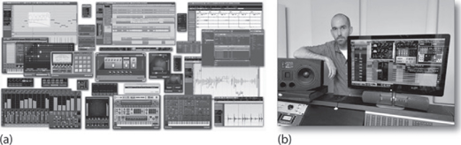
FIGURE 15.3
Signal processing plug-ins. (a) Collage of the various screens within the Cubase media production DAW.(Courtesy of Steinberg Media Technologies GmbH, www.steinberg.net) (b) Producer/engineer Billy Bush mixing Garbage’s “Not Your Kind of People” with Universal Audio’s Apollo and UAD2 accelerated plug-ins. (Photo courtesy of Universal Audio/David Goggin, www.uaudio.com)
Plug-In Control and Automation
A fun and powerful aspect of working with various signal processing plug-ins on a DAW platform is the ability to control and automate many or all of the various effects parameters with relative ease and recall. These controls can be manipulated on-screen (via hands-on or track parameter controls) or from an external hardware controller (Figure 15.4), allowing the parameters to be physically controlled in real time.

FIGURE 15.4
External EFX hardware controllers. (a) Novation’s Nocturn automatically maps its controls to various parameters on the target plug-in. (Courtesy of Novation Digital Music Systems, Ltd., www.novationmusic.com) (b) Native Instruments Komplete Kontrol system maps instruments and plug-ins to its hardware controls. (Courtesy of Native Instruments GmbH, www.native-instruments.com)
SIGNAL PATHS IN EFFECTS PROCESSING
Before diving into the process of effecting and/or altering sound, we should first take a quick look at an important signal path concept—the fact that a signal processing device can be inserted into an analog, digital or DAW chain in several ways. The most common of these are:
■ Insert routing
■ Send routing
Insert Routing
Insert routing is often used to alter the sonic or effects characteristics of a single track or channel signal. It occurs whenever a processor is directly inserted into a signal path in a serial (pass thru) fashion. Using this approach, the audio source enters into the input path, passes through the inserted signal processor and then continues on to carry out the record, monitor and/or mix function.
This method of inserting a device is generally used for the processing of a single instrument, voice or grouped set of signals that are present on a particular hardware or virtual input strip. Often, but not always, the device tends to be an amplitude-based processing function (such as an equalizer, compressor or limiter). In keeping with the “no-rules” concept, however, time- and pitch-changing devices can also be used to tweak an instrument or voice as an insert. Here are but a few examples of how an insert can be used:
■ A device can be plugged into an input strip’s insert (direct send/return) point. This approach is used to insert an outboard device directly into the input signal path of an analog, digital or DAW strip (Figure 15.5a).
■ A processor (such as a stereo compressor, limiter, EQ, etc.) could be inserted into a mixer’s main output bus to affect an overall mix.
■ A processor (such as a stereo compressor, limiter, EQ, etc.) could be inserted into a grouping to affect a sub-mix.
■ An effects stomp box could be inserted between a mic preamp and console input to create a grungy distortion effect.
■ A DAW plug-in could be inserted into a strip to process only the signal on that channel (Figure 15.5b).
An insert is used to “insert” an effect or effects chain into a single track or group. It tends (but not always), to be amplitude-based in nature, meaning the processor is often used to effect amplitude levels (i.e., compressor, limiter, gate, etc.)

FIGURE 15.5
Inserting an effect into a channel strip. (a) Analog insert. (b) DAW insert.
EXTERNAL CONTROL OVER AN INSERT EFFECT’S SIGNAL PATH
Certain insert effects processors allow for an external audio source to act as a control for affecting a signal as it passes from the input to the output of a device (Figure 15.6). Devices that offer an external “key” or “sidechain” input can be quite useful, allowing a signal source to be used as a control for varying another audio path. For example:
■ A gate (an infinite expander that can control the passing of audio through a gain device) might take its control input from an external “key” signal that will determine when a signal will or will not pass in order to reduce leakage, tighten up an instrument decay or to create an effect.
■ A vocal track could be inserted into a vocoder’s control input, so as to synthetically add a robot-like effect to a track.
■ A voice track could be used for vocal ducking at a radio station, as a control to fade out the music or crowd noise when a narrator is speaking.
■ An external keyed input can be used to make a mix “pump” or “breathe” in a dance production.

FIGURE 15.6
Diagram of a key side-chain input to a noise gate. (a) The signal is passed whenever a signal is present at the key input. (b) No signal is passed when no signal is present at the key input.
It’s important to note that there is no set standard for providing a side-chain key in software. Some software packages provide native side-chain capability, others support side-chaining via “multiple input” plug-ins and complex signal routing and many don’t support side-chaining at all.
Send Routing
Effects “sends” are often used to augment a signal (generally being used to add reverb, delay or other time-based effects). This type differs from an insert, in that instead of inserting a signal-changing device directly into the signal path, a portion of the signal (which is essentially a combined mix of the desired channels) is then “sent” to one or more effects devices. Once effected, the signal can then be proportionately mixed back into the monitor or main out signal path, so as to add an effects blend of the selected tracks to the overall output mix.
A send is used to “send” a mix of multiple channel signals to a single effect or effects chain, after which, it is routed to the monitor or main mix bus. It tends (but not always) to be time-based in nature, meaning the processor effects time functions (i.e., reverb, echo, etc.)
As an example, Figure 15.7 shows how sends from any number of channel inputs can be mixed together and then be sent to an effects device. The effected output signal is then sent back into either the effects return section or to a set of spare mixer inputs or directly to the main mixing bus outputs.

FIGURE 15.7
An “aux” sends path flows in a horizontal fashion to a send bus. The combined sum can then be effected (or sent to another destination) and the returned back to the monitor or main output bus. (a) Analog aux send. (b) Digital aux send.
Viva La Difference
There are a few insights that can help you to understand the difference between insert and send effects routing. Let’s start by reviewing the basic ways that their signal paths function:
■ First, from Figure 15.5, we can see that the signal flow of an effects insert is basically “vertical,” moving from the channel input through an inserted device and then back into the input strip’s signal chain (for mixing, recording or whatever).
■ From Figure 15.7 we can see that an effects send basically functions in a “horizontal” direction, allowing portions of the various input signals to be mixed together and sent to an effects device, whic can then be routed back into the mixer signal chain for further effects and mix blending.
■ Finally, it’s important to grasp the idea that when a device is “inserted” into a signal chain, it’s usually a single, dedicated hardware/plug-in device (or sometimes chain of devices) that is used to perform a specific function. If a large number of track/channels are used in a session or mix, inserting numerous DSP effects into multiple strips could take up too much processing power (or are simply unnecessary and hard to manage). Setting up an effects send can save a great deal of DSP processing overhead by creating a single effects send “mix” that can then be routed to a single effects device (or device chain)—it works like this: “why use a whole bunch of EFX devices to do the same job on every channel, when sending a signal mix to a single EFX device/chain will do.”
On a final note, each effects routing technique has its own set of strengths and weaknesses—it’s important to play with each, so as to know the difference and when to make best use of each of them.
SIDE CHAIN PROCESSING
Another effects processing tool that can be used to add “character” to your mix is the idea of side chain processing. Essentially, side chain processing (also known as parallel processing) is a fancy word for setting up a special effects send and return that can add a degree of spice to your overall mix. It could quite easily be:
■ A processing chain that adds varying degrees of compression, tape saturation and/or distortion to add a bit of “grunge” to the mix (Figure 15.8).
■ A send mix that is routed to loud guitar amp in the studio (or amp simulation plug-in) that is being picked up by several close and distant room mics to add character to the mix.
■ A room simulation plug-in to add space to an otherwise lifeless mix.

FIGURE 15.8
An example of how side chain processing can add a bit of character to a mix.
The options and possible effects combinations are endless. By naming the send “glue,” “dirt” “grit” or anything you want, a degree of character that is uniquely yours can be added to the mix. I’d like to add a bit of caution here, however: Adding grit to your mix can be all well and good (especially if it’s a rock track that just begs for some extra dirt). However, it’s also possible to overdo it by adding too much distortion into the mix. Too much of a good thing is just that—too much.
There is one more control that you should be aware of. A number of hardware and plug-in devices have an internal “wet/dry mix” control that serves as an internal side-chain mix control for varying the amount of “dry” (original) signal to be mixed with the “wet” (effected) signal (usually varied in percentage). This setting can have an effect on your settings (when used in either an insert or send setting) and a careful awareness is advised.
EFFECTS PROCESSING
From this point on, this chapter will be taking an in-depth look at many of the signal processing devices, applications and techniques that have traditionally been the cornerstone of music and sound production, including systems and techniques that exert an ever-increasing degree of control over:
■ The spectral content of a sound: In the form of equalization and bandpass filtering
■ Amplitude level processing: In the form of dynamic range processing
■ Time-based effects: Augmentation or re-creation of room ambience, delay, time/pitch alterations and tons of other special effects that can range from being sublimely subtle to “in yo’ face.”
Hardware and Plug-In Effects in Action
The following sections offer some insight into the basics of effects processing and how they can be integrated into a recording or mixdown. It’s a forgone conclusion that the power of these effects can be harnessed in hardware or software plug-in form. An important rule to remember is that there are no rules; however, there are a few general guidelines that can help you get the sound that you want. When using effects, the most important asset you can have is experience and your own sense of artistry. The best way to learn the art of processing, shaping and augmenting sound is through experience; gaining that takes time and patience.
EQUALIZATION
An audio equalizer (Figure 15.9) is a circuit, device or plug-in that lets us exert control over the harmonic or timbral content of a recorded sound. EQ may need to be applied to a single recorded channel, to a group of channels or to an entire program.
Equalization refers to the alteration in frequency response of an amplifier so that the relative levels of certain frequencies are more or less pronounced than others. EQ is specified as either plus or minus a certain number of decibels at a certain frequency. For example, you might want to boost a signal by “+4 dB at 5 kHz.” Although only one frequency was specified in this example, in reality a range of frequencies above, below and centered around the specified frequency will actually be affected. The amount of boost or cut at frequencies other than the one named is determined by whether the curve is peaking or shelving, by the bandwidth of the curve (a factor that’s affected by the Q settings and determines how many frequencies will be affected around a chosen centerline), and by the amount of boost or cut at the named frequency. For example, a +4 dB boost at 1000 Hz might easily add a degree of boost or cut at 800 and 1200 Hz (Figure 15.10).
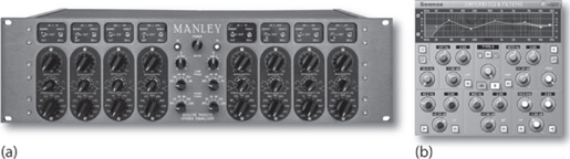
FIGURE 15.9
The audio equalizer. (a) Manley Massive Passive Analog Stereo Equalizer. (Courtesy of Manley Laboratories, Inc., www.manleylabs.com) (b) Sonnox Oxford EQ. (Courtesy of Universal Audio, www.uaudio.com. ©) 2017 Universal Audio, Inc. All rights reserved. Used with permission)

FIGURE 15.10
Various boost/cut EQ curves centered around 1 kHz: (a) center frequency, 1-kHz bandwidth 1 octave, ±15 dB boost/cut; (b) center frequency, 1 kHz bandwidth 3 octaves, ±15 dB boost/cut.
Older equalizers and newer “retro” systems often base their design around filters that use passive components (i.e., inductors, capacitors and resistors) and employ amplifiers only to make up for internal losses in level, called insertion loss. Most equalization circuits today, however, are of the active filter type that change their characteristics by altering the feedback loop of an operational amp. This is by far the most common analog EQ type and is generally favored over its passive counterpart due to its low cost, size and weight, as well as its wide gain range and line-driving capabilities.
Peaking Filters
The most common EQ curve is created by a peaking filter. As its name implies, a peak-shaped bell curve can either be boosted or cut around a selected center frequency. Figure 15.11a shows the curves for a peak equalizer that’s set to boost or cut at 1000 Hz. The quality, factor (Q) of a peaking equalizer refers to the width of its bell-shaped curve. A curve with a high Q will have a narrow bandwidth with few frequencies outside the selected bandwidth being affected, whereas a curve having a low Q is very broadband and can affect many frequencies (or even octaves) around the center frequency. Bandwidth is a measure of the range of frequencies that lie between the upper and lower –3-dB (half-power) points on the curve (Figure 15.11b). The Q of a filter is an inverse measure of the bandwidth (such that higher Q values mean that fewer frequencies will be affected, and vice versa). To calculate Q, simply divide the center frequency by the bandwidth. For example, a filter centered at 1 kHz that’s a third of an octave wide will have its –3 dB frequency points located at 891 and 1123 Hz, yielding a bandwidth of 232 Hz (1123—891). This EQ curve’s Q, therefore, will be 1 kHz divided by 232 Hz or 4.31.

FIGURE 15.11
Peaking equalization curves. (a) Various Q widths. (b) The number of hertz between the two points that are 3 dB down from the center frequency determines the bandwidth of a peaking filter.
Shelving Filters
Another type of equalizer is the shelving filter. Shelving refers to a rise or drop in frequency response at a selected frequency, which tapers off to a preset level and continues at that level to the end of the audio spectrum. Shelving can be inserted at either the high or low end of the audio range and is the curve type that’s commonly found on home stereo bass and treble controls (Figure 15.12).

FIGURE 15.12
High/low, boost/cut curves of a shelving equalizer.
High-Pass and Low-Pass Filters
Equalizer types also include high-pass and low-pass filters. As their names imply, this EQ type allows certain frequency bandwidths to be passed at full level while other sections of the audible spectrum are attenuated. Frequencies that are attenuated by less than 3 dB are said to be inside the passband; those attenuated by more than 3 dB are located outside, in the stopband. The frequency at which the signal is attenuated by exactly 3 dB is called the turnover or cutoff frequency and is used to name the filter frequency.
Ideally, attenuation would become infinite immediately outside the passband; however, in practice this isn’t always attainable. Commonly, attenuation is carried out at rates of 6, 12 and 18 dB per octave. This rate is called the slope of the filter. Figure 15.13a, for example, shows a 700-Hz high-pass filter response curve with a slope of 6 dB per octave, and Figure 15.13b shows a 700-Hz low-pass filter response curve having a slope of 12 dB per octave. High- and low-pass filters differ from shelving EQ in that their attenuation doesn’t level off outside the passband. Instead, the cutoff attenuation continues to increase. A high-pass filter in combination with a low-pass filter can be used to create a bandpass filter, with the passband being controlled by their respective turnover frequencies and the Q by the filter’s slope (Figure 15.14).

FIGURE 15.13
A 700-Hz filter: (a) high-pass filter with a slope of 6 dB per octave; (b) low-pass filter with a slope of 12 dB per octave.

FIGURE 15.14
A bandpass filter is created by combining a high- and low-pass filter with different cutoff frequencies.
Equalizer Types
The four most commonly used equalizer types that can incorporate one or more of the previously described filter types are the:
■ Selectable frequency equalizer
■ Parametric equalizer
■ Graphic equalizer
■ Notch filter
The selectable frequency equalizer (Figure 15.15), as its name implies, has a set number of frequencies from which to choose. These equalizers usually allow a boost or cut to be performed at a number of selected frequencies with a predetermined Q. They are most often found on older console designs, certain low-cost production consoles and outboard gear.

FIGURE 15.15
The Warm Audio EQP-WA selectable frequency tube equalizer. (Courtesy of Warm Audio LLC, www.warmaudio.com)
The parametric equalizer (Figure 15.16a) lets you adjust most or all of its frequency parameters in a continuously variable fashion. Although the basic design layout will change from model to model, each band will often have an adjustment for continuously varying the center frequency. The amount of boost or cut is also continuously variable. Control over the center frequency and Q can be either selectable or continuously variable, although certain manufacturers might not have provisions for a variable Q.
Generally, each set of frequency bands will overlap into the next band section, so as to provide smooth transitions between frequency bands or allow for multiple curves to be placed in nearby frequency ranges. Because of its flexibility and performance, the parametric equalizer has become the standard design for most input strips, digital equalizers and workstations.
A graphic equalizer (Figure 15.16b) provides boost and cut level control over a series of center frequencies that are equally spaced (ideally according to music intervals). An “octave band” graphic equalizer might, for example, have 12 equalization controls spaced at the octave intervals of 20, 40, 80, 160, 320 and 640 Hz and 1.25, 2.5, 5, 10 and 20 kHz, while 1/3-octave equalizers could have up to 36 center frequency controls. The various EQ band controls generally use vertical sliders that are arranged side by side so that the physical positions of these controls could provide a “graphic” readout of the overall frequency response curve at a glance. This type is often used in applications that can help fine-tune a system to compensate for the acoustics in various types of rooms, auditoriums and studio control rooms.
Notch filters are often used to zero in on and remove 60- or 50-Hz hum or other undesirable discrete-frequency noises. They use a very narrow bandwidth to fine-tune and attenuate a particular frequency in such a way as to have little effect on the rest of the audio program. Notch filters are used more in film location sound and broadcast than in studio recording, because severe narrowband problems aren’t often encountered in a well-designed studio—hopefully.

FIGURE 15.16
Equalizer types: (a) the EQF-100 full range, parametric vacuum tube equalizer. (Courtesy of Summit Audio, Inc., www.summitaudio.com);(b) Rane GE 130 single-channel, 30-band, 1/3-octave graphic equalizer. (Courtesy of Rane Corporation, www.rane.com)
Applying Equalization
When you get right down to it, EQ is all about compensating for deficiencies in a sound pickup or about reducing extraneous sounds that make their way into a pickup signal. To start our discussion on how to apply EQ, let’s again revisit the all-important “Good Rule” from Chapter 4.
The “Good Rule”
Good musician + good instrument + good performance + good acoustics + good mic + good placement = good sound.
Whenever possible, EQ should not be used as a Band-Aid. By this, I mean that it’s often a good idea to correct for a problem on the spot rather than to rely on the hope that you can “fix it in the mix” at a later time using EQ and other methods.
When in doubt, it’s often better to deal with a problem as it occurs. This isn’t always possible, however—therefore, EQ is best used in situations where:
■ There’s no time or money left to redo the track
■ The existing take was simply magical and shouldn’t be re-recorded
■ The track was already recorded during a previous session and is in need of being fixed.
EQ in Action!
Although most equalization is done by ear, it’s helpful to have a sense of which frequencies affect an instrument in order to achieve a particular effect. On the whole, the audio spectrum can be divided into four frequency bands: low (20 to 200 Hz), low-mid (200 to 1000 Hz), high-mid (1000 to 5000 Hz) and high (5000 to 20,000 Hz). When the frequencies in the 20- to 200-Hz (low) range are modified, the fundamental and the lower harmonic range of most bass information will be affected. These sounds often are felt as well as heard, so boosting in this range can add a greater sense of power or punch to music. Lowering this range will weaken or thin out the lower frequency range.
The fundamental notes of most instruments lie within the 200- to 1000-Hz (low-mid) range. Changes in this range often result in dramatic variations in the signal’s overall energy and add to the overall impact of a program. Because of the ear’s sensitivity in this range, a minor change can result in an effect that’s very audible. The frequencies around 200 Hz can add a greater feeling of warmth to the bass without loss of definition. Frequencies in the 500- to 1000-Hz range could make an instrument sound hornlike, while too much boost in this range can cause listening fatigue.
Higher-pitched instruments are most often affected in the 1000 to 5000 Hz (high-mid) range. Boosting these frequencies often results in an added sense of clarity, definition and brightness. Too much boost in the 1000 to 2000 Hz range can have a “tinny” effect on the overall sound, while the upper mid-frequency range (2000 to 4000 Hz) affects the intelligibility of speech. Boosting in this range can make music seem closer to the listener, but too much of a boost can also cause listening fatigue.
The 5000–20,000 Hz (high-frequency) region is composed almost entirely of instrument harmonics. For example, boosting frequencies in this range will often add sparkle and brilliance to a string or woodwind instrument. Boosting too much might produce sibilance on vocals and make the upper range of certain percussion instruments sound harsh and brittle. Boosting at around 5000 Hz has the effect of making music sound louder. A 6 dB boost at 5000 Hz, for example, can sometimes make the overall program level sound as though it’s been doubled in level; conversely, attenuation can make music seem more distant. Table 15.1 provides an analysis of how frequencies and EQ settings can interact with various instruments. (For more information, refer to the Microphone Placement Techniques section in Chapter 4.)
Table 15.1 Instrumental Frequency Ranges of Interest
| Instrument | Frequencies of Interest |
| Kick drum | Bottom depth at 60–80 Hz, slap attack at 2.5 kHz |
| Snare drum | Fatness at 240 Hz, crispness at 5 kHz |
| Hi-hat/cymbals | Clank or gong sound at 200 Hz, shimmer at 7.5 kHz to 12 kHz |
| Rack toms | Fullness at 240 Hz, attack at 5 kHz |
| Floor toms | Fullness at 80–120 Hz, attack at 5 kHz |
| Bass guitar | Bottom at 60–80 Hz, attack/pluck at 700–1000 Hz, string noise/pop at 2.5 kHz |
| Electric guitar | Fullness at 240 Hz, bite at 2.5 kHz |
| Acoustic guitar | Bottom at 80–120 Hz, body at 240 Hz, clarity at 2.5–5 kHz |
| Electric organ | Bottom at 80–120 Hz, body at 240 Hz, presence at 2.5 kHz |
| Acoustic piano | Bottom at 80–120 Hz, presence at 2.5–5 kHz, crisp attack at 10 kHz, honky-tonk sound (sharp Q) at 2.5 kHz |
| Horns | Fullness at 120–240 Hz, shrill at 5–7.5 kHz |
| Strings | Fullness at 240 Hz, scratchiness at 7.5–10 kHz |
| Conga/bongo | Resonance at 200–240 Hz, presence/slap at 5 kHz |
| Vocals | Fullness at 120 Hz, boominess at 200–240 Hz, presence at 5 kHz, sibilance at 7.5–10 kHz |
Note: These frequencies aren’t absolute for all instruments, but are meant as a subjective guide.
Try This: Equalization
1. Solo an input strip on a mixer, console or DAW. Experiment with the settings using the previous frequency ranges. Can you improve on the original recorded track or does it take away from the sound?
2. Using the input strip equalizers on a mixer, console or DAW, experiment with the EQ settings and relative instrument levels within an entire mix using the previous frequency ranges as a guide. Can you bring an instrument out without changing the fader gains? Can you alter the settings of two or more instruments to increase the mix’s overall clarity?
3. Plug an outboard or plug-in equalizer into the main output buses of a mixer, console or DAW, change the program’s EQ settings using the previous frequency range discussions as a guide. How does it change the mix?
One way to zero in on a particular frequency using an equalizer (especially a parametric one) is to accentuate or attenuate the EQ level and then vary the center frequency until the desired range is found. The level should then be scaled back until the desired effect is obtained. If boosting in one-instrument range causes you to want to do the same in other frequency ranges, it’s likely that you’re simply overdoing it. It’s easy to get caught up in the “bigger! Better! MORE!” syndrome of wanting an instrument to sound louder. If this continues to happen on a mix, it’s likely that one of the frequency ranges of an instrument or ensemble is too dominant and requires attenuation. On the subject of laying down a recorded track with EQ, there are a number of situations and differing opinions regarding them:
■ Some will “track” (record) the sound the mic/instrument/room sound directly to tape or disk, so that little or no EQ (or any other changes) will be needed in mixdown.
■ Some use EQ liberally to make up for placement and mic deficiencies, whereas others might use it sparingly, if at all. One example where EQ is used sparingly is when an engineer knows that someone else will be mixing a particular song or project. In this situation, the engineer who’s doing the mix might have a very different idea of how an instrument should sound. If large amounts of EQ were recorded to a track during the session, the mix engineer might have to work very hard to counteract the original EQ settings.
■ If everything was recorded flat, the producer and artists might havedifficulty passing judgment on a performance or hearing the proper balance during the overdub phase. Such a situation might call for equalization in the monitor mix, while leaving the recorded tracks alone.
■ In situations where several mics are to be combined onto a single track or channel, the mics can only be individually equalized (exchanged, altered or moved) during the recording phase. In situations where a project is to be engineered, mixed and possibly even mastered by the same person, the engineer might want to discuss in advance the type and amount of EQ that the producer and/or artist might want.
■ Above all, it’s wise that any “sound-shaping” should be determined and discussed with the producer and/or artist before the sounds are committed to a track.
In the end, there’s no getting around the fact that an equalizer is a powerful tool. When used properly, it can greatly enhance or restore the musical and sonic balance of a signal. Experimentation and experience are the keys to proper EQ usage, and no book can replace the trial-and-error process of “just doing it!”
Before moving on, it’s important to keep one age-old viewpoint in mind—that an equalizer shouldn’t be regarded as a cure-all for improper mic, playing or instrument technique; rather, it should be used as a tool for correcting problems that couldn’t be easily fixed on the spot through mic and/or performance adjustments. If an instrument is poorly recorded during an initial recording session, it’s often far more difficult and time consuming to “fix it in the mix” at a later time. Getting the best possible sound down onto tape or DAW will definitely improve your chances for attaining a sound and overall mix that you can be proud of in the future.
Sound-Shaping Effects Devices and Plug-Ins
Another class of effects devices that aren’t equalizers, but instead affect the overall tonal character of a track or mix come under the category of sound-shaping devices. These systems can either be hardware or plug-in in nature and are used to alter the tonal and/or overtone balance of a signal. For example, a device that’s been around for decades in the Aphex Aural Exiter. This device is able to add a sense of presence to a sound by generating additional overtones that are subdued or not present in the program signal. Other such devices are able to modify the shape of a sounds transient envelope (Figure 5.17a) or to filter the sound in unique ways (Figure 5.17b).

FIGURE 15.17
Sound-shaping plug-ins. (a) Oxford Envolution. (b) Moog multimode filter. (Courtesy of Universal Audio, www.uaudio.com. © 2017 Universal Audio, Inc. All rights reserved. Used with permission)

FIGURE 15.18
Analog tape emulation plug-in. (a) Oxide Tape Recorder for the Apollo and the UAD effects processing card. (Courtesy of Universal Audio, www.uaudio.com © 2017 Universal Audio, Inc. All rights reserved. Used with permission) (b) Slate Digital Virtual Tape Machine. (Courtesy of Slate Digital, www.slatedigital.com)
Another class of sound-shaper comes in the form of virtual tape machine plug-ins that closely model and emulate analog tape recorders—right down to their sonic character, tape noise, distortion, changes with virtual tape formulation and bias settings (Figure 15.18).
DYNAMIC RANGE
Like most things in life that get out of hand from time to time, the level of a signal can vary widely from one moment to the next. For example, if a vocalist gets caught up in the moment and lets out an impassioned scream following a soft whispery passage, you can almost guarantee that the mic and preamp will push the recording chain from its optimum recording level into severe distortion—OUCH! Conversely, if you set an instrument’s mic to properly accommodate the loudest level, its signal might be buried in the mix during the rest of the song. For these and other reasons, it becomes obvious that it’s sometimes necessary to exert some form of control over a signal’s dynamic range by using various techniques and dynamic controlling devices. In short, the dynamics of an audio program’s signal resides somewhere in a continuously varying realm between three level states:
■ Saturation
■ Average signal level
■ System/ambient noise
As you may remember from various chapters in this book that saturation occurs when an input signal is so large that an amp’s supply voltage isn’t large enough to produce the required output current or is so large that a digital converter reaches full scale (where the A/D output reads as all 1’s). In either case, the results generally don’t sound pretty and should be avoided in the channel’s audio chain. The average signal level is where the overall signal level of a mix often likes to reside. Logically, if an instrument’s level is too low, it can get buried in the mix—if it’s too high, it can unnecessarily stick out and throw the entire balance off. It is here that the art of creating an average mix level that’s high enough to stand out in any playlist, while still retaining enough dynamic “life,” truly becomes an applied balance of skill and magic.
DYNAMIC RANGE PROCESSORS
The overall dynamic range of music is potentially on the order of 120 to 140 dB, whereas the overall dynamic range of a compact disc is often 80 to 90 dB, and analog magnetic tape is on the order of 60 dB (excluding the use of noise-reduction systems, which can improve this figure by 15 to 30 dB). However, when working with 24-bit digital word lengths, a system, processor or channel’s overall dynamic range can actually approach or exceed the full range of hearing. Even with such a wide dynamic range, unless the recorded program is played back in a noise-free environment, either the quiet passages will get lost in the ambient noise of the listening area (35 to 45 dB SPL for the average home and much worse in a car) or the loud passages will simply be too loud to bear. Similarly, if a program of wide dynamic range were to be played through a medium with a limited dynamic range (such as the 20- to 30-dB range of an AM radio or the 40- to 50-dB range of FM), a great deal of information would get lost in the general background noise. To prevent such problems, the dynamics of a program can be restricted to a level that’s appropriate for the reproduction medium (theater, radio, home system, car, etc.) as shown in Figure 15.19. This gain reduction can be accomplished either by manually riding the fader’s gain or through the use of a dynamic range processor that can alter the range between the signal’s softest and loudest passages.
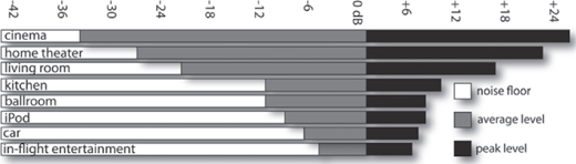
FIGURE 15.19
Dynamic ranges of various audio media, showing the noise floor (black), average level (white) and peak levels (gray). (Courtesy of Thomas Lund, tc electronic, www.tcelectronic.com)
The concept of automatically changing the gain of an audio signal (through the use of compression, limiting and/or expansion) is perhaps one of the most misunderstood aspects of audio recording. This can be partially attributed to the fact that a well-done job won’t be overly obvious to the listener. Changing the dynamics of a track or overall program will often affect the way in which it will be perceived (either consciously or unconsciously) by making it “seem” louder, thereby reducing its volume range to better suit a particular medium or by making it possible for a particular sound to ride at a better level above other tracks within a mix.
COMPRESSION
A compressor (Figure 15.20), in effect, can be thought of as an automatic fader. It is used to proportionately reduce the dynamics of a signal that rises above a user-definable level (known as the threshold) to a lesser volume range. This process is done so that:
■ The dynamics can be managed by the electronics and/or amplifiers in the signal chain without distorting the signal chain.
■ The range is appropriate to the overall dynamics of a playback or broadcast medium.
■ An instrument or vocal better matches the dynamics of other recorded tracks within a song or audio program.

FIGURE 15.20
Universal Audio 1176LN limiting amplifier. (Courtesy of Universal Audio, www.uaudio.com. © 2017 Universal Audio, Inc. All rights reserved. Used with permission)
Since the signals of a track, group or program will be automatically turned down (hence the terms compressed or squashed) during a loud passage, the overall level of the newly reduced signal can now be amplified upwards to better fit into a mix or to match the required dynamics of the medium. In other words, once the dynamics have been reduced downward, the overall level can be boosted such that the range between the loud and soft levels is less pronounced (Figure 15.21). We’ve not only restored the louder signals back to a prominent level but we have also turned up the softer signals that would otherwise be buried in the mix or ambient background noise.

FIGURE 15.21
A compressor reduces input levels that exceed a selected threshold by a specified amount. Once reduced, the overall signal can then be boosted in level, thereby allowing the softer signals to be raised above other program or background sounds.
The most common controls on a compressor (and most other dynamic range devices) include input gain, threshold, output gain, slope ratio, attack, release and meter display:
■ Input gain: This control is used to determine how much signal will be sent to the compressor’s input stage.
■ Threshold: This setting determines the level at which the compressor will begin to proportionately reduce the incoming signal. For example, if the threshold is set to –20 dB, all signals that fall below this level will be unaffected, while signals above this level will be proportionately attenuated, thereby reducing the overall dynamics. On some devices, varying the input gain will correspondingly control the threshold level. In this situation, raising the input level will lower the threshold point and thus reduce the overall dynamic range. Most quality compressors offer hard and soft knee threshold options. A soft knee widens or broadens the threshold range, making the onset of compression less obtrusive, while the hard knee setting causes the effect to kick in quickly above the threshold point.
■ Output gain: This control is used to determine how much signal will be sent to the device’s output. It’s used to boost the reduced dynamic signal into a range where it can best match the level of a medium or be better heard in a mix.
■ Slope ratio: This control determines the slope of the input-to-output gain ratio. In simpler terms, it determines the amount of input signal (in decibels) that’s needed to cause a 1 dB increase at the compressor’s output. For example, linear amplifier has an input-to-output ratio of 1:1 (one-to-one), meaning for every 1 dB increase at the input, there will be a corresponding 1 dB increase at the output (Figure 15.22a). When using a 2:1 compression ratio, below the threshold the signal will be linear (1:1), however, above this level an increase of 2 dB will result in an increase of only 1 dB at the output (Figure 15.22b). An increase of 4 dB above the threshold will result in an output gain of 1 dB, when a 4:1 ratio (slope) is selected. Get the idea?
■ Attack: This setting (which is calibrated in milliseconds; 1 msec = 1 thousandth of a second) determines how fast or how slowly the device will turn down signals that exceed the threshold. It is defined as the time it takes for the gain to decrease to a percentage (usually 63%) of its final gain value. In certain situations (as might occur with instruments that have a long sustain, such as the bass guitar), setting a compressor to instantly turn down a signal might be audible (possibly creating a sound that pumps the signal’s dynamics). In this situation, it would be best to use a slower attack setting. On the other hand, such a setting might not give the compressor time to react to sharp, transient sounds (such as a hi-hat). In this case, a fast attack time would probably work better. As you might expect, you’ll need to experiment to arrive at the fastest attack setting that won’t audibly color the signal’s sound.

FIGURE 15.22
The output ratios of a compressor. (a) A liner slope results in an increase of 1 dB at the output for every 1 dB increase at the input. (b) A compression slope follows an input/output gain reduction ratio above the threshold, proportionately reducing signals that fall above this point.
■ Release: Similar to the attack setting, release (which is calibrated in milli-seconds) is used to determine how slowly or quickly the device will restore a signal to its original dynamic level once it has fallen below the threshold point (defined as the time required for the gain to return to 63% of its original value). Too fast a setting will cause the compressor to change dynamics too quickly (creating an audible pumping sound), while too slow a setting might affect the dynamics during the transition from a loud to a softer passage. Again, it’s best to experiment with this setting to arrive at the slowest possible release that won’t color the signal’s sound.
■ Meter display: This control changes the compressor’s meter display to read the device’s output or gain reduction levels. In some designs, there’s no need for a display switch, as readouts are used to simultaneously display output and gain reduction levels.
As was previously stated, the use of compression (and most forms of dynamics processing) is often misunderstood, and compression can easily be abused. Generally, the idea behind these processing systems is to reduce the overall dynamic range of a track, music or sound program or to raise its overall perceived level without adversely affecting the sound of the track itself. It’s a well-known fact that over-compression can actually squeeze the life out of a performance by limiting the dynamics and reducing the transient peaks that can give life to a performance. For this reason, it’s important to be aware of the general nuances of the controls that have been discussed.
During a recording or mixdown session, compression can be used in order to balance the dynamics of a track to the overall mix or to keep the signals from overloading preamps, the recording medium and your ears. Compression should be used with care for any of the following reasons:
■ Minimize changes in volume that might occur whenever the dynamics of an instrument or vocal are too wide for the mix. As a tip, a good starting point might be a 0 dB threshold setting at a 4:1 ratio, with the attack and release controls set at their middle positions.
■ Smooth out momentary changes in source-to-mic distance.
■ Balance out the volume ranges of a single instrument. For example, the notes of an electric or upright bass often vary in volume from string to string. Compression can be used to “smooth out” the bass line by matching their relative volumes (often using a slow attack setting). In addition, some instruments (such as horns) are louder in certain registers because of the amount of effort that’s required to produce these notes. Compression is often useful for smoothing out these volume changes. As a tip, you might start with a ratio of 5:1 with a medium-threshold setting, medium attack and slower release time. Over-compression should be avoided to avoid pumping effects.
■ Reduce other frequency bands by inserting a filter into the compression chain that causes the circuit to compress frequencies in a specific band (multi-band compression). A common example of this is a deesser, which is used to detect high frequencies in a compressor’s circuit so as to suppress those “SSSS,” “CHHH” and “FFFF” sounds that can distort or stand out in a recording.
■ Reduce the dynamic range and/or boost the average volume of a mix so that it appears to be significantly louder (as occurs when a song’s volume sticks out in a playlist or a television commercial seems louder than your favorite show).
Although it may not always be the most important, this last application often gets a great deal of attention, because many producers strive to cut their recordings as “hot” as possible. That is, they want the recorded levels to be as far above the normal operating level as possible without blatantly distorting. In this competitive business, the underlying logic behind the concept is that louder recordings (when placed into a Top 40, podcast, phone or MP3 playlist) will stand out from the softer recordings and get noticed. In fact, reducing the dynamic range of a song or program’s dynamic range will actually make the overall levels appear to be louder. By using a slight (or not-so-slight) amount of compression and limiting to squeeze an extra 1 or 2 dB gain out of a song, the increased gain will also add to the perceived bass and highs because of our ears’ increased sensitivity at louder levels (remember the Fletcher-Munson curve discussed in Chapter 2?). To achieve these hot levels without distortion, multiband compressors and limiters often are used during the mastering process to remove peaks and to raise the average level of the program. You’ll find more on this subject in Chapter 20 (Mastering).
Compressing a mono mix is done in much the same way as one might compress a single instrument—although greater care should be taken. Adjusting the threshold, attack, release and ratio controls are more critical in order to prevent “pumping” sounds or loss of transients (resulting is a lifeless mix). Compressing a stereo mix gives rise to an additional problem: If two independent compressors are used, a peak in one channel will only reduce the gain on that channel and will cause sounds that are centered in a stereo image to shift (or jump) toward the channel that’s not being compressed (since it will actually be louder). To avoid this center shifting, most compressors (of the same make and model) can be linked as a stereo pair. This procedure of ganging the two channels together interconnects the signal-level sensing circuits in such a way that a gain reduction in one channel will cause an equal reduction in the other.
Before moving on, let’s take a look at a few examples of the use of compression in various applications. Keep in mind, these are only beginning suggestions— nothing can substitute for experimenting and finding the settings that work best for you and the situation:
■ Acoustic guitar: A moderate degree of compression (3 to 8 dB) with a medium compression ratio can help to pull an acoustic forward in a mix. A slower attack time will allow the string’s percussive attack to pass through.
■ Bass guitar: The electric bass is often a foundation instrument in pop and rock music. Due to variations in note levels from one note to another on an electric bass guitar (or upright acoustic, for that matter), a compressor can be used to even out the notes and add a bit of presence and/or punch to the instrument. Since the instrument often (but not always) has a slower attack, it’s often a good idea to start with a medium attack (4:1, for example) and threshold setting, along with a slower release time setting. Harder compression of up to 10:1 with gain reductions ranging from 5 to 10 dB can also give a good result.
■ Brass: The use of a faster attack (1 to 5 ms) with ratios that range from 6:1 to 15:1 and moderate to heavy gain reduction can help keep the brass in line.
■ Electric guitar: In general, an electric guitar won’t need much compression, because the sound is often evened out by the amp, the instrument’s natural sustain character and processing pedals. If desired, a heavier compression ratio, with 10 or more decibels of compression can add to the instrument’s “bite” in a mix. A faster attack time with a longer release is often a good place to start.
■ Kick drum and snare: These driving instruments often benefit from added compression. For the kick, a 4:1 ratio with an attack setting of 10 ms or slower can help emphasize the initial attack while adding depth and presence. The snare attack settings might be faster, so as to catch the initial transients. Threshold settings should be set for a minimum amount of reduction during a quiet passage, with larger amounts of gain reduction happening during louder sections.
■ Synths: These instruments generally don’t vary widely in dynamic range, and thus won’t require much (or any) compression. If needed, a 4:1 ratio with moderate settings can help keep synth levels in check.
■ Vocals: Singers (especially inexperienced ones) will often place the mic close to their mouths. This can cause wide volume swings that change with small moves in distance. The singer might also shout out a line just after delivering a much quieter passage. These and other situations lead to the careful need for a compressor, so as to smooth out variations in level. A good starting point would be a threshold setting of 0 dB, with a ratio of 4:1 with attack and release settings set at their midpoints. Gain reductions that fall between 3 and 6 dB will often sit well in a mix (although some rock vocalists will want greater compression) be careful of over-compression and its adverse pumping artifacts. Given digital’s wide dynamic range, you might consider adding compression later in the mixdown phase, rather than during the actual session.
■ Final mix compression: It’s often a common practice to compress an entire mix during mixdown. If the track is to be professionally mastered, you should consult with the mastering engineer before the deed is done (or you might provide him or her with both a compressed and uncompressed version). When applying bus compression, it is usually a good idea to start with medium attack and release settings, with a light compression ratio (say, 4:1). With these or your preferred settings, reduce the threshold detection until a light amount of compression is seen on the meter display. Levels of between 3 and 6 dB will provide a decent amount of compression without audible pumping or artifacts (given that a well-designed unit or plug-in is used).
Try This: Compression
1. Go to the Tutorial section of www.modrec.com and download the tutorial sound files that relate to compression (which include instrument/music segments in various dynamic states).
2. Listen to the tracks. If you have access to an editor or DAW, import the files and look at the waveform amplitudes for each example. If you’d like to DIY, then:
3. Record or obtain an uncompressed bass guitar track and monitor it through a compressor or compression plug-in. Increase the threshold level until the compressor begins to kick in. Can you hear a difference? Can you see a difference on the console or mixer meters?
4. Set the levels and threshold to a level you like and then set the attack time to a slow setting. Now, select a faster setting and continue until it sounds natural. Try setting the release to its fastest setting. Does it sound better or worse? Now select a slower setting. Does it sound more natural?
5. Repeat the above routine and settings using a snare drum track. Were your findings any different?
Multiband compression
Multiband compression (Figure 15.23) works by breaking up the audible spectrum into various frequency bandwidths through the use of multiple bandpass filters. This allows each of the bands to be isolated and processed in ways that strictly minimize the problems or maximize the benefits in a particular band. Although this process is commonly done in the final mastering stage, multiband techniques can also be used on an instrument or grouping. For example:

FIGURE 15.23
Multiband compressors. (a) Universal Audio’s UAD Precision Multiband plug-in. (Courtesy of Universal Audio, www.uaudio.com. © 2017 Universal Audio, Inc. All rights reserved. Used with permission) (b) Steinberg multiband compressor. (Courtesy of Steinberg Media Technologies GmbH, a division of Yamaha Corporation, www.steinberg.net)
■ The dynamic upper range of a slap bass could be lightly compressed, while heavier amounts of compression could be applied to the instrument’s lower register.
■ An instrument’s high end can be brightened simply by adding a small amount of compression. This can act as a treble boost while reducing any sharp attacks that might jump out in a mix.
LIMITING
If the compression ratio is made large enough, a compressor will actually become a limiter. A limiter (Figure 15.24) is used to keep signal peaks from exceeding a specified level in order to prevent the overloading of amplifier signals, recorded signals onto tape or disc, broadcast transmission signals, and so on. Most limiters have ratios of 10:1 (above the threshold, for every 10 dB increase at the input there will be a gain of 1 dB at the output) or 20:1 (Figure 15.25), although some have ratios that can range up to 100:1. Since a large increase above the threshold at the input will result in a very small increase at its output, the likelihood of overloading any equipment that follows the limiter will be greatly reduced. Limiters have three common functions:
■ To prevent signal levels from increasing beyond a specified level: Certain types of audio equipment (often those used in broadcast transmission) are often designed to operate at or near their peak output levels. Significantly increasing these levels beyond 100% would severely distort the signal and possibly damage the equipment. In these cases, a limiter can be used to prevent signals from significantly increasing beyond a specified output level.
■ To prevent short-term peaks from reducing a program’s average signal level: Should even a single high-level peak exist at levels above the program’s rms average, the overall level can be significantly reduced. This is especially true whenever a digital audio file is normalized at any percentage value, because the peak level will become the normalized maximum value and not the average level. Should only a few peaks exist in the file, they can easily be zoomed in on and manually reduced in level. If multiple peaks exist, then a limiter should be considered.

FIGURE 15.24
Limiter plug-ins. (a) Waves L1 Ultramaximizer limiting/quantization plug-in. (Courtesy of Waves Ltd., www.waves.com) (b) Universal Audio’s UAD Precision Limiter plug-in. (Courtesy of Universal Audio, www.uaudio.com. © 2017 Universal Audio, Inc. All rights reserved. Used with permission)

FIGURE 15.25
The output ratios of a limiter. (a) A liner slope results in an increase of 1 dB at the output for every 1 dB increase at the input. (b) A limiter slope follows a very high input/output gain reduction ratio (10:1, 20:1 or more) above the threshold, proportionately “limiting” signal level, so that they do not increase above a set point.
■ To prevent high-level, high-frequency peaks from distorting analog tape: When recording to certain media (such as cassette and videotape), high-energy, transient signals actually don’t significantly add to the program’s level however, if allowed to pass, these transients can easily result in distortion or tape saturation.
Unlike the compression process, extremely short attack and release times are often used to quickly limit fast transients and to prevent the signal from being audibly pumped. Limiting a signal during the recording and/or mastering phase should only be used to remove occasional high-level peaks, as excessive use would trigger the process on successive peaks and would be noticeable. If the program contains too many peaks, it’s probably a good idea to reduce the level to a point where only occasional extreme peaks can be detected.
EXPANSION
Expansion is the process by which the dynamic range of a signal is proportionately increased. Depending on the system’s design, an expander (Figure 15.26) can operate either by decreasing the gain of a signal (as its level falls below the threshold) or by increasing the gain (as the level rises above it). Most expanders are of the first type, in that as the signal level falls below the expansion threshold the gain is proportionately decreased (according to the slope ratio), thereby increasing the signal’s overall dynamic range (Figure 15.27). These devices can also be used as noise reducers. You can do this by adjusting the device so that the noise is downwardly expanded during quiet passages, while louder program levels are unaffected or only moderately reduced. As with any dynamics device, the attack and release settings should be carefully set to best match the program material. For example, choosing a fast release time for an instrument that has a long sustain can lead to audible pumping effects. Conversely, slow release times on a fast-paced, transient instrument could cause the dynamics to return to its linear state more slowly than would be natural. As always, the best road toward understanding this and other dynamics processes is through experimentation.
Try This: Limiting
1. Go to the Tutorial section of www.modrec.com, click on limiting and download the sound files (which include instrument/music segments in various states of limiting).
2. Listen to the tracks. If you have access to an editor or DAW, import the files and look at the waveform amplitudes for each example. If you’d like to DIY, then:
3. Feed an isolated track or entire mix through a limiter or limiting plug-in.
4. With the limiter switched out, turn the signal up until the meter begins to peg (you might want to turn the monitors down a bit).
5. Now reduce the level and turn it up again—this time with the limiter switched in. Is there a point where the level stops increasing, even though you’ve increased the input signal? What does the gain reduction meter show? Decrease and increase the threshold level and experiment with the signal’s dynamics. What did you find out?
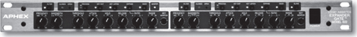
FIGURE 15.26
The Aphex Model 622 Logic-Assisted Expander/Gate. (Courtesy of Aphex Systems, Inc., www.aphex.com

FIGURE 15.27
Commonly, the output of an expander is linear above the threshold and follows a low input/output gain expansion ratio below this point.
THE NOISE GATE
One other type of expansion device is the noise gate (Figure 15.28). This device allows a signal above a selected threshold to pass through to the output at unity gain (1:1) and without dynamic processing; however, once the input signal falls below this threshold level, the gate acts as an infinite expander and effectively mutes the signal by fully attenuating it. In this way, the desired signal is allowed to pass while background sounds, instrument buzzes, leakage or other unwanted noises that occurs between pauses in the music are muted. Here are a few examples of where a noise gate might be used:
■ To reduce leakage between instruments. Often, parts of a drum kit fall into this category; for example, a gate can be used on a high-tom track in order to reduce excessive leakage from the snare.
■ To eliminate tape or system noise from an instrument or vocal track during silent passages.
FIGURE 15.28
Noise gates are commonly included within many dynamic plug-in processors. (a) Noise Gate Plug-in. (Courtesy of Avid Technology, Inc., www.avid.com) (b) Noise Gate Plug-in. (Courtesy of Steinberg Media Technologies GmbH, a division of Yamaha Corporation, www.steinberg.net) (c) Noise Gate found on Duality console. (Courtesy of Solid State Logic, www.solid-state-logic.com)
The general rules of attack and release apply to gating as well. Fortunately, these settings are a bit more obvious during the gating process than with any other dynamic tool. Improperly set attack and release times will often be immediately obvious when you’re listening to the instrument or vocal track (either on its own or within a mix) because the sound will cut in and out at inappropriate times.
Commonly, a key input (as previously shown in Figure 15.6) is included as a side-chain path for triggering a noise gate. A key input is an external control that allows an external analog signal source (such as a miked instrument or signal generator) to trigger the gate’s audio output path. For example, a mic or recorded track of a kick drum could be used to key a low-frequency oscillator. Whenever the kick sounds, the oscillator will be passed through the gate. By combining the two, you can have a deep kick sound that’ll make the room shake, rattle and roll.
Time-Based Effects
Another important effects category that can be used to alter or augment a signal revolves around delays and regeneration of sound over time. These time-based effects often add a perceived depth to a signal or change the way we perceive the dimensional space of a recorded sound. Although a wide range of time-based effects exist, they are all based on the use of delay (and/or regenerated delay) to achieve such results as:
■ Time-delay or regenerated echoes, chorus and flanging
■ Reverb
DELAY
One of the most common effects used in audio production today alters the parameter of time by introducing various forms of delay into the signal path. Creating a delay circuit is a relatively simple task to accomplish digitally. Although dedicated delay devices (often referred to as digital delay lines, or DDLs) are readily available on the market, most multifunction signal processors and time-related plug-ins are capable of creating this straightforward effect (Figure 15.29). In its basic form, digital delay is accomplished by storing sampled audio directly into RAM. After a defined length of time (usually measured in milliseconds), the sampled audio can be read out from memory for further processing or direct output (Figure 15.30a). Using this basic concept, a wide range of effects can be created simply by assembling circuits and program algorithms into blocks that can introduce delays or regenerated echo loops. Of course, these circuits will vary in complexity as new processing blocks are introduced.
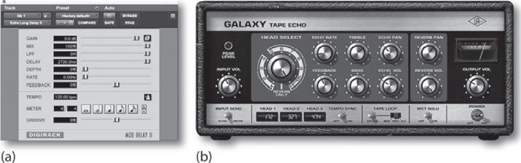
FIGURE 15.29
Delay plug-ins. (a) Pro Tools Mod Delay II. (Courtesy of Avid Technology, Inc., www.avid.com) (b) Galaxy Tape Echo Plug-in. (Courtesy of Universal Audio, www.uaudio.com. © 2017 Universal Audio, Inc. All rights reserved. Used with permission)
Delay in Action: Less than 15 ms
Probably the best place to start looking at the delay process is at the sample level. By introducing delays downward into the microsecond (one millionth of a second) range, control over a signal’s phase characteristics can be introduced to the point where selective equalization actually begins to occur. In reality, controlling very short-term delays is actually how EQ is carried out in both the analog and digital domains!
Whenever delays that fall below the 15-ms range are slowly varied over time and then are mixed with the original undelayed signal, an effect known as combing is created. Combing is the result of changes that occur when equalized peaks and dips appear in the signal’s frequency response. By either manually or automatically varying the time of one or more of these short-term delays, a constantly shifting series of effects known as flanging can be created. Depending on the application, this effect (which makes a unique “swishing” sound that’s often heard on guitars or vocals) can range from being relatively subtle to having moderate to wild shifts in time and pitch. It’s interesting to note the differences between the effects of phasing and flanging. Phasing uses all-pass filters to create uneven peaks and notches, whereas flanging uses delay lines to create even peaks and notches although, the results are somewhat similar.
Delay in Action: 15 to 35 ms
By combining two identical (and often slightly delayed) signals that are slightly detuned in pitch from one another, an effect known as chorusing can be created. Chorusing is an effects tool that’s often used by guitarists, vocalists and other musicians to add depth, richness and harmonic structure to their sound. Increasing delay times into the 15- to 35-ms range will create signals that are spaced too closely together to be perceived by the listener as being discrete delays. Instead, these closely spaced delays create a doubling effect when mixed with an instrument or group of instruments (Figure 15.30b). In this instance, the delays actually fool the brain into thinking that more instruments are playing than actually are—subjectively increasing the sound’s density and richness. This effect can be used on background vocals, horns, string sections and other grouped instruments to make the ensemble sound as though it has doubled (or even tripled) its actual size. This effect also can be used on foreground tracks, such as vocals or instrument solos, to create a larger, richer and fuller sound. Some “chorus” delay devices introduce slight changes in delay and pitch shifting, allowing for detunings that can create an interesting, humanized sound.

FIGURE 15.30
Digital delay. (a) A ddl stores sampled audio into RAM, where it can be read out at a later time. (b) In certain instances, ddl (doubling or double delay) can fool the brain into thinking that more instruments are playing than actually are.
Should time or budget be an issue, it’s also possible to create this doubling effect by actually recording a second pass to a new set of tracks. Using this method, a 10-piece string section could be made to sound like a much larger ensemble. In addition, this process automatically gives vocals, strings, keyboards and other legato instruments a more natural effect than the one you get by using an electronic effects device. This having been said, these devices can actually go a long way toward duplicating the effect. Some delay devices even introduce slight changes in delay times in order to create a more natural, humanized sound. As always, the method you choose will be determined by your style, your budget and the needs of your particular project.
Delay in Action: More than 35 ms
When the delay time is increased beyond the 35- to 40-ms point, the listener will begin to perceive the sound as being a discrete echo. When mixed with the original signal, this effect can add depth and richness to an instrument or range of instruments that can really add interest to an instrument within a mix.
Adding delays to an instrument that are tied to the tempo of a song can go even further toward adding a degree of depth and complexity to a mix. Most delay-based plug-ins make it easy to insert tempo-based delays into a track. For hardware delay devices, it’s usually necessary to calculate the tempo math that’s required to match the session. Here’s the simple math for making these calculations:
60,000/tempo = time (in ms)
For example, if a song’s tempo is 100 bpm (beats per minute), then the amount of delay needed to match the tempo at the beat level would be:
60,000/100 = 600 ms
Using divisions of this figure (300, 150, 75, etc.) would insert delays at 1/2, 1/4, 1/8 measure intervals.
Caution should be exercised when adding delay to an entire musical program, because the program could easily begin to sound muddy and unintelligible. By feeding the delayed signal back into the circuit, a repeated series of echo … echo … echoes can be made to simulate the delays of yesteryear—you’ll definitely notice that Elvis is still in the house.
REVERB
In professional audio production, natural acoustic reverberation is an extremely important tool for the enhancement of music and sound production. A properly designed acoustical environment can add a sense of space and natural depth to a recorded sound that’ll often affect the performance as well as its overall sonic character. In situations where there is little, no or substandard natural ambience, a high-quality reverb device or plug-in (Figure 15.31) can be extremely helpful in filling the production out and giving it a sense of dimensional space and perceived warmth. In fact, reverb consists of closely spaced and random multiple echoes that are reflected from one boundary to another within a determined space (Figure 15.32). This effect helps give us perceptible cues as to the size, density and nature of a space (even though it might have been artificially generated). These cues can be broken down into three subcomponents:
Try This: Delay
1. Go to the Tutorial section of www.modrec.com and download the delay tutorial sound files (which include segments with varying degrees of delay).
2. Listen to the tracks. If you’d like to DIY, then:
3. Insert a digital delay unit or plug-in into a program channel and balance the dry track’s output-mix, so that the input signal is set equally with the delayed output signal. (Note: If there is no mix control, route the delay unit’s output to another input strip and combine delayed/undelayed signals at the console.)
4. Listen to the track with the mix set to listen equally to the dry and effected signal.
5. Vary the settings over the 1- to 10-ms range. Can you hear any rough EQ effects?
6. Manually vary the settings over the 10- to 35-ms range. Can you simulate a rough phasing effect?
7. Increase the settings above 35 ms. Can you hear the discrete delays?
8. If the unit has a phaser setting, turn it on. How does it sound different?
9. Now change the delay settings a little faster to create a wacky flange effect. If the unit has a flange setting, turn it on. Try playing with the time-based settings that affect its sweep rate. Fun, huh?
■ Direct signal
■ Early reflections
■ Reverberation
The direct signal is heard when the original sound wave travels directly from the source to the listener. Early reflections is the term given to those first few reflections that bounce back to the listener from large, primary boundaries in a given space. Generally, these reflections are the ones that give us subconscious cues as to the perception of size and space. The last set of reflections makes up the signal’s reverberation characteristic. These sounds are comprised of zillions of random reflections that travel from boundary to boundary within the confines of a room. These reflections are so closely spaced in time that the brain can’t discern them as individual reflections, so they’re perceived as a single, densely decaying signal.
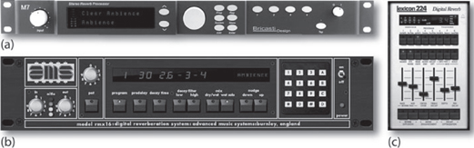
FIGURE 15.31
Digital reverb effects processors. (a) Bricasti M7 Stereo Reverb Processor. (Courtesy of Bricasti Design Ltd, www.bracasti.com) (b and c) AMS rmx16 and EMT 140 reverb plug-ins for the Apollo and the UAD effects processing card. (Courtesy of Universal Audio, www.uaudio.com © 2017 Universal Audio, Inc. All rights reserved. Used with permission)

FIGURE 15.32
Signal level versus reverb time.
Reverb Types
By varying program and setting parameters, a digital reverb device can be used to simulate a wide range of acoustic environments, reverb devices and special effects. A few popular categories include:
■ Hall: Simulates the acoustics of a concert hall. This is often a diffuse, lush setting with a longer RT60 decay time (the time that’s required for a sound to decay by 60 dB).
■ Chamber: Simulates the acoustics of an echo chamber. Like a live chamber, these settings often simulate the brighter reflectivity of tile or cement surfaces.
■ Room: As you might expect, these settings simulate the acoustics of a midto large-sized room. It’s often best suited to intimate solo instruments or a chamber atmosphere.
■ Live (stage): Simulates a live performance stage. These settings can vary widely but often simulate long early-delay reflections.
■ Spring: Simulates the low-fidelity “boingyness” of yesteryear’s spring reverb devices.
■ Plate: Simulates the often-bright diffuse character of yesteryear’s metallic plate reverb devices. These settings are often used on vocals and percussion instruments.
■ Reverse: These backward-sounding effects are created by reversing the decay trail’s envelope so that the decay increases in level over time and is quickly cut off at the tail end, yielding a sudden break effect. This can also be realistically created in a DAW by reversing a track or segment, applying reverb, and then reversing it again to yield a true backward reverb trail.
■ Gate: Cuts off the decay trail of a reverb signal. These settings are often used for emphasis on drums and percussion instruments.
Try This: Reverb Types
1. Open up a DAW session that contains various instruments (such as a snare, guitar and vocal).
2. Insert (or send) a reverb plug-in into each track.
3. Listen to each track, while changing the plug-in presets between “hall,” “plate,” “small room,” etc. How do they sound different? Do they sound different for each instrument?
PSYCHOACOUSTIC ENHANCEMENT
A number of signal processors rely on psychoacoustic cues in order to fool the brain into perceiving a particular effect. The earliest and most common of these devices are those that enhance the overall presence of a signal or entire recording by synthesizing upper-range frequency harmonics and inserting them into a mix in order to brighten the perceived sound. Although the additional harmonics won’t significantly affect the program’s overall volume, the effect is a marked increase in its perceived presence. Other psychoacoustic devices that make use of complex harmonic, phase, delay and equalization parameters have become standard production tools in the field of mastering in order to shape the final sound into one that’s interesting, with a sonic character all their own.
In addition to synthesizing harmonics in order to change or enhance a recording or track, other digital psychoacoustic processors deal exclusively with the subject of spatialization (the placement of an audio signal within a three-dimensional acoustic field), even though the recording is being played back over stereo speakers. By varying the parameters of a stereo or multiple input source, this processing function creates phase and amplitude paths that can fool the brain into perceiving that the stereo image is actually emanating from a sound field that’s wider than the physical speaker positions. In practice, care should be taken when using these devices, because the effect is often carried off with degrees of success that vary from system to system. In addition, the use of phase relationships to expand the stereo sound field can actually cause obvious cancellation problems when the program is listened to in mono.
PITCH SHIFTING
Ever had a perfectly good vocal take that was spoiled by just one or two flat notes? Or had a project come in the door with a guitar track that was out of tune? Or needed to change the key on a 30-second radio spot? It’s times like these that pitch shifting can save your day! Pitch shifting can be used to vary the pitch of a signal or sound file (either upward or downward) in order to transpose the relative pitch of an audio program without affecting its duration. This process can take place in either real time or non-real time. Pitch shifting works by writing sampled audio data to a temporary memory, where it’s resampled to either a higher or a lower sample rate (according to the desired final pitch). Once this is done, the processor either adds interpolated samples to (lowers the pitch) or subtracts them from (raises the pitch) the resampled data to return it back to the original output rate, while keeping the altered pitch intact. Figure 15.33 gives two basic examples of how this is often carried out.

FIGURE 15.33
Two pitch-shift examples with an initial 1-kHz digital signal and a sample rate of 44.1 kHz: (a) The signal can be halved in pitch (to 500 Hz) by internally downsampling to a new rate of 22.05 k. To return the output rate to 44.1 (while retaining the 500-Hz pitch), new sample points must be added into each dropped position. (b) The signal can be doubled in pitch (to 2 kHz) by internally upsampling to a new rate of 88.2 k. To return the output rate to 44.1 (while retaining the 2-kHz pitch), every other sample point must be dropped.
A degree of caution should be used when changing the pitch of a program or audio segment. Whenever uneven or minute interval changes are made, the interpolation of samples doesn’t always fall perfectly into place. This can lead to digital artifacts that adds amounts of harmonic distortion that can range from slightly noticeable to unacceptable. If the track is in the background, there shouldn’t be a problem; however, care should be taken with upfront instruments and vocals. It’s important to keep in mind that large pitch changes might be more noticeable. As always, your ears are the best judge.
Time and Pitch Changes
By combining variable sample rates and pitch shifting techniques, it’s possible to create three different variations:
■ Time change: A program’s length can be altered, without affecting its pitch, by raising or lowering its playback sample rate.
■ Pitch change: A program’s length can remain the same while pitch is shifted either up or down.
■ Both: Both a program’s pitch and length can be altered by means of simple resampling techniques.
These functions have become an important part of the signal processing and music production arsenals that are used by the audio-for-video, film and broadcast industries. They help give producers control over the running time of film video and audio soundtracks while maintaining the original, natural pitch of voice, music and effects. For example, using a DAW, we could add 5 seconds onto the end of an existing 25-second public service radio spot simply by time shifting the 25-second spot to 30 seconds (while keeping the pitch intact).
In addition to the basic time/pitch techniques that are commonly used in music production (most often by electronic musicians), this technology has allowed for the huge explosion in loop-based music composition and production. These popular programs and music plug-ins involve the use of recorded sound files that are encoded with headers that include information on their native tempo and length (in both samples and beats). When you set the loop program to a master tempo (or a specific tempo at that point in the score), a loop segment, once imported, can go about the process of recalculating its pitch and tempo to match the current session tempo and—voilà! The file’s in sync with the song! Further info on loop-based production tools can be found in Chapter 8 (Groove Tools and Techniques).
It’s important to realize that the algorithms that control how time and pitch are to be calculate differ between programs (as well as having various algorithm options within the same program). It would be wise to read up on how your favorite programs deal with these shifting techniques (or better yet, listen to various percussion and pad-based loops) and then familiarize yourself with how the different algorithms sound. The quality of your sound files will thank you.
Automatic Pitch Correction
One other pitch correction category makes use of auto-tuning software or plug-ins that are able to automatically detect off-tune or slight pitch-bend segments of a track and then correct these inaccuracies (according to user parameters). These systems (Figure 15.34) are commonly used in modern music production in situations that range from:
■ Simple track pitch corrections to fix the overall tuning of a track.
■ Automated and manual micro-tuning to correct bad or out-of-tune notes in a vocal or instrument performance.
■ Using parameters that fix tuning steps that can create an absolutely “perfect” performance.

FIGURE 15.34
Automatic pitch correction software. (a) Melodyne Editor auto pitch correction system. (Courtesy of Celemony Software GmbH, www.celemony.com). (b) Auto-Tune pitch correction system. (Courtesy of Antares Audio Technologies, www.antarestech.com)
■ Creating an extreme tuning effect that exaggerates the various tuning steps in pitch to give a non-human, robotic-like effect to a vocal or instrumental performance
Often, these pitch editors allow us to change the pitch in a straightforward, graphical environment, according to musical and/or user-defined parameters. Single notes or entire chords can be built up, altered or changed, making it possible to correct a wide range of material. It’s even possible to alter individual notes within a polyphonic recording. For example, you could fix a single wrong note in a piano recording or change the notes within a guitar backing track— all after the recording has been made. In short, automatic pitch correction has become practically an art in itself, and several have made a career out of it. Of course, there is too much to fully cover the nuances and intricacies of pitch correction here, fortunately, there are hundreds (maybe thousands) of video tutorials on the subject. Dive into them, then dive into the software—experiment and have fun!
Of course, the use of automatic tuning to fix a track isn’t without its critics. In 1998 Cher released one of the first popular songs with Auto-Tune Believe, and since then, pitch correction has become a mainstream tool for pop, country, hip hop, you-name-it. As a tool, pitch correction can be carefully used to make a vocal or track sound more in tune, to many, it’s use (some would say, overuse) takes away from the artistry and humanity of a performance. As with most tools of the effects trade, it’s wise to take the time to become familiar with the details, depth and consequences of pitch correction and then talk with the musicians and producer about their intentions.
MULTIPLE-EFFECTS DEVICES
Since most digital signal processors are by nature multifunctional chameleons, it follows that most hardware and certain plug-in processors can be easily programmed to perform various functions. For this reason, many digital systems have been designed to perform as multiple-effects devices (Figure 15.35). Multiple effects, in this case, can have several basic meanings:

FIGURE 15.35
Multi-effects processing devices. (a) Controller for tc electronic System 6000 digital effects processor. (Courtesy of tc electronic, www.tcelectronic.com) (b) Lexicon 224 reverb plug-in for the Apollo and the UAD effects processing card. (Courtesy of Universal Audio, www.uaudio.com © 2017 Universal Audio, Inc. All rights reserved. Used with permission)
■ A single device might offer a wide range of processing functions but allow only one effect to be called up at a time.
■ A single device might offer a range of processing functions that can be “stacked” to perform a number of simultaneous effects.
■ An effects device might have multiple ins and outs, each of which can perform several processing functions (effectively giving you multiple processors that can be used in a multichannel mixdown environment).
DYNAMIC EFFECTS AUTOMATION AND EDITING
One of the joys of working with effects is the ability to manipulate and vary effects parameters in real time over the duration of a song or audio program. By altering parameters, changing settings and mixing effects levels—the subtle variations in expression can add a great deal of interest to a project.
The ability to dynamically automate effects settings can be accomplished in any number of ways, including:
■ Via MIDI control and parameter change messages
■ Via external hardware controller
■ Via DAW automation or other form of automation control
In closing, an almost unlimited degree of effects control is available to us through most high-level (and many entry-level) digital audio workstations. Through the use of any of the readily available hardware controllers or on-screen automation controls, it’s possible to manipulate and automate effects within a DAW session with an amazing degree of sophistication and ease.
Go ahead, get hold of these fun and effective tools and experiment your heart out!
Try This: DAW Effects Automation
The vast majority of plug-in effects can be directly and dynamically automated within the computer’s DAW program. It’s my greatest hope that you’ll:
■ Take a look at your favorite DAW manual and start reading!
■ Open up a tutorial session or better yet, make your own.
■ Call up some effects on various tracks.
■ Call up some automation control parameters and start grabbing controls.
■ Learn how to edit these automation functions, so as to be able to finesse your effects in new and interesting ways.