Chapter Five

Extrapolation Algorithms

5.1 INTRODUCTION

The standard PageRank algorithm uses the Power Method to compute successive iterates that converge to the principal eigenvector of the Markov matrix A representing the Web link graph. Since it was shown in the previous chapter that the Power Method converges quickly, one approach to accelerating PageRank would be to directly modify the Power Method to exploit our knowledge about the matrix A.

In this chapter, we present several algorithms that accelerate the convergence of PageRank by using successive iterates of the Power Method to estimate the nonprincipal eigenvectors of A, and periodically subtracting these estimates from the current iterate x^(k) of the Power method. We call this class of algorithms extrapolation algorithms. We present three extrapolation algorithms in this chapter: Aitken Extrapolation and Quadratic Extrapolation exploit our knowledge that the first eigenvalue λ₁(A) = 1, and Power Extrapolation exploits our knowledge from the previous chapter that λ2(A) = c.

Empirically, we show that Quadratic Extrapolation and Power Extrapolation speed up PageRank computation by 25–300% on a Web graph of 80 million nodes, with minimal overhead. This contribution is useful to the PageRank community and the numerical linear algebra community in general, as these are fast methods for determining the dominant eigenvector of a Markov matrix that is too large for standard fast methods to be practical.

5.2 AITKEN EXTRAPOLATION

5.2.1 Formulation

We begin by introducing Aitken Extrapolation, which we develop as follows. We assume that the iterate can be expressed as a linear combination of the first two eigenvectors. This assumption allows us to solve for the principal eigenvector in closed form using the successive iterates .

Of course, can only be approximated as a linear combination of the first two eigenvectors, so the that we compute is only an estimate of the true However, it can be seen from Section 2.3.1 that this approximation becomes increasingly accurate as k becomes larger.

We begin our formulation of Aitken Extrapolation by assuming that can be expressed as a linear combination of the first two eigenvectors

Since the first eigenvalue λ₁ of a Markov matrix is 1, we can write the next two iterates as

Now, let us define

where x_i represents the ith component of the vector . Doing simple algebra using (5.2) and (5.3) gives

Now, let us define f_i as the quotient g_i/h_i:

Therefore,

Hence, from (5.1), we have a closed-form solution for :

However, since this solution is based on the assumption that can be written as a linear combination of and , (5.11) gives only an approximation to . Algorithms 3 and 4 show how to use Aitken Extrapolation in conjunction with the Power Method to get consistently better estimates of .

Aitken Extrapolation is equivalent to applying the well-known Aitken Δ² method for accelerating linearly convergent sequences [4] to each component of the iterate . What is novel here is this derivation of Aitken acceleration, and the proof that Aitken acceleration computes the principal eigenvector of a Markov matrix in one step under the assumption that the power-iteration estimate can be expressed as a linear combination of the first two eigenvectors.

As a sidenote, let us briefly develop a related method. Rather than using (5.4), let us define gi alternatively as

We define h as in (5.5), and f_i now becomes

Algorithm 3: Aitken Extrapolation

Algorithm 4: Power Method with Aitken Extrapolation

By (5.2),

Again, this is an approximation to , since it is based on the assumption that can be expressed as a linear combination of and . What is interesting here is that this is equivalent to performing a second-order epsilon acceleration algorithm [73] on each component of the iterate . For this reason, we call this algorithm Epsilon Extrapolation. In experiments, Epsilon Extrapolation has performed similarly to Aitken Extrapolation, so we will focus on Aitken Extrapolation in the next sections.

5.2.2 Operation Count

In order for an extrapolation method such as Aitken Extrapolation or Epsilon Extrapolation to be useful, the overhead should be minimal. By overhead, we mean any costs in addition to the cost of applying Algorithm 1 to generate iterates. It is clear from inspection that the operation count of the loop in Algorithm 3 is O(n), where n is the number of pages on the Web. The operation count of one extrapolation step is less than the operation count of a single iteration of the Power Method, and since Aitken Extrapolation may be applied only periodically, we say that Aitken Extrapolation has minimal overhead. In our implementation, the additional cost of each application of Aitken Extrapolation was negligible—about 1% of the cost of a single iteration of the Power Method (i.e., 1% of the cost of Algorithm 1).

Figure 5.1 Comparison of convergence rate for unaccelerated Power Method and Aitken Extrapolation on the STANFORD.EDU dataset, for c = 0.99. Extrapolation was applied at the 10th iteration.

5.2.3 Experimental Results

In Figure 5.1, we show the convergence of the Power Method with Aitken Extrapolation applied once at the 10th iteration, compared to the convergence of the unaccelerated Power Method for the STANFORD.EDU dataset. The x-axis denotes the number of. times a multiplication A occurred, that is, the number of times Algorithm 1 was needed. Note that there is a spike at the acceleration step, but speedup occurs nevertheless. This spike is caused by the poor approximation for . The speedup likely occurs because, while the extrapolation step introduces some error in the components in the direction of each eigenvector, it is likely to actually reduce the error in the component in the direction of the second eigenvector, which is slow to go away by the standard Power Method.

Multiple applications of Aitken Extrapolation are generally not more useful than only one. This is because, by the time the residual settles down from the first application, a second extrapolation approximation does not give a very different estimate from the current iterate itself.

For c = 0.99, Aitken Extrapolation takes 38% less time to reach an iterate with a residual of 0.01. However, after this initial speedup, the convergence rate for Aitken slows down, so that to reach an iterate with a residual of 0.002, the time savings drops to 13%. For lower values of c, Aitken provides much less benefit. Since there is a spike in the residual graph, if Aitken Extrapolation is applied too often, the power iterations will not converge. In experiments, Epsilon Extrapolation performed similarly to Aitken Extrapolation.

5.2.4 Discussion

The methods presented thus far are very different from standard fast eigensolvers, which generally rely strongly on matrix factorizations or matrix inversions. Standard fast eigensolvers do not work well for the PageRank problem, since the Web hyperlink matrix is so large and sparse. For problems where the matrix is small enough for an efficient inversion, standard eigensolvers such as inverse iteration are likely to be faster than these methods. The Aitken and Epsilon Extrapolation methods take advantage of the fact that the first eigenvalue of the Markov hyperlink matrix is 1 to find an approximation to the principal eigenvector.

In the next section, we present Quadratic Extrapolation, which assumes the iterate can be expressed as a linear combination of the first three eigenvectors, and solves for in closed form under this assumption. As we shall soon discuss, the Quadratic Extrapolation step is simply a linear combination of successive iterates, and thus does not produce spikes in the residual.

5.3 QUADRATIC EXTRAPOLATION

5.3.1 Formulation

We develop the Quadratic Extrapolation algorithm as follows. We assume that the Markov matrix A has only 3 eigenvectors, and that the iterate can be expressed as a linear combination of these 3 eigenvectors. These assumptions allow us to solve for the principal eigenvector in closed form using the successive iterates

Of course, A has more than 3 eigenvectors, and can only be approximated as a linear combination of the first 3 eigenvectors. Therefore, the that we compute in this algorithm is only an estimate for the true . We show empirically that this estimate is a better estimate to than the iterate , and that our estimate becomes closer to the true value of as k becomes larger. In Section 5.3.3 we show that by periodically applying Quadratic Extrapolation to the successive iterates computed in PageRank, for values of c close to 1, we can speed up the convergence of PageRank by a factor of over 3.

We begin our formulation with the assumption stated at the beginning of this section

We then define the successive iterates

Since we assume A has 3 eigenvectors, the characteristic polynomial p_A(λ) is given by

A is a Markov matrix, so we know that the first eigenvalue λ₁ = 1. The eigenvalues of A are also the zeros of the characteristic polynomial p_A(λ). Therefore,

The Cayley-Hamilton theorem states that any matrix A satisfies its own characteristic polynomial p_A(A) = 0 [30]. Therefore, by the Cayley-Hamilton theorem, for any vector z in

Letting , we have

From (5.13)–(5.15),

From (5.17),

We may rewrite this as

Let us make the following definitions:

We can now write (5.22) in matrix notation:

We now wish to solve for . Since we are not interested in the trivial solution , we constrain the leading term of the characteristic polynomial :

We may do this because constraining a single coefficient of the polynomial does not affect the zeros.¹ (5.26) is therefore written

This is an overdetermined system, so we solve the corresponding least-squares problem,

where Y⁺ is the pseudoinverse of the matrix . Now, (5.17), (5.27), and (5.29) completely determine the coefficients of the characteristic polynomial p_A(λ) (5.16).

Algorithm 5: Quadratic Extrapolation

We may now divide p_A(λ) by λ − 1 to get the polynomial q_A(λ), whose roots are λ₂ and λ₃, the second two eigenvalues of A

Simple polynomial division gives the following values for β₀,β₁, and β₂:

Again, by the Cayley-Hamilton theorem, if z is any vector in

where is the eigenvector of A corresponding to eigenvalue 1 (the principal eigenvector). Letting , we have

From (5.13)–(5.15), we get a closed form solution for :

However, since this solution is based on the assumption that A has only 3 eigenvectors, (5.36) gives only an approximation to .

Algorithms 5 and 6 show how to use Quadratic Extrapolation in conjunction with the Power Method to get consistently better estimates of .

Algorithm 6: Power Method with Quadratic Extrapolation

1. Compute the reduced QR factorization Y = QR using 2 steps of Gram-Schmidt.

2. Compute the vector – Q^Ty^(k).

3. Solve the upper triangular system:

Algorithm 7: Using Gram-Schmidt to solve for γ₁ and γ₂

5.3.2 Operation Count

The overhead in performing the extrapolation shown in Algorithm 5 comes primarily from the least-squares computation of γ₁ and γ₂:

It is clear that the other steps in this algorithm are either O(1) or O(n) operations.

Since Y is an n × 2 matrix, we can do the least-squares solution cheaply in just 2 iterations of the Gram-Schmidt algorithm [68]. Therefore, γ₁ and γ₂ can be computed in O(n) operations. While a presentation of Gram-Schmidt is outside the scope of this book, we show in Algorithm 7 how to apply Gram-Schmidt to solve for [γ₁γ₂]^T in O(n) operations. Since the extrapolation step is on the order of a single iteration of the Power Method, and since Quadratic Extrapolation is applied only periodically during the Power Method, we say that Quadratic Extrapolation has low overhead. In our experimental setup, the overhead of a single application of Quadratic Extrapolation is half the cost of a standard power iteration (i.e., half the cost of Algorithm 1). This number includes the cost of storing on disk the intermediate data required by Quadratic Extrapolation (such as the previous iterates), since they may not fit in main memory.

5.3.3 Experimental Results

Of the algorithms we have discussed for accelerating the convergence of PageRank, Quadratic Extrapolation performs the best empirically. In particular, Quadratic Extrapolation considerably improves convergence relative to the Power Method when the damping factor c is close to 1. We measured the performance of Quadratic Extrapolation under various scenarios on the LARGEWEB dataset. Figure 5.2 shows the rates of convergence when c = 0.90; after factoring in overhead, Quadratic Extrapolation reduces the time needed to reach a residual of 0.001 by 23%.² Figure 5.3 shows the rates of convergence when c = 0.95; in this case, Quadratic Extrapolation speeds up convergence more significantly, saving 31% in the time needed to reach a residual of 0.001. Finally, in the case where c = 0.99, the speedup is more dramatic. Figure 5.4 shows the rates of convergence of the Power Method and Quadratic Extrapolation for c = 0.99. Because the Power Method is so slow to converge in this case, we plot the curves until a residual of 0.01 is reached. The use of extrapolation saves 69% in time needed to reach a residual of 0.01; that is, the unaccelerated Power Method took more than three times as long as the Quadratic Extrapolation method to reach the desired residual. The wallclock times for these scenarios are summarized in Figure 5.5.

Figure 5.2 Comparison of convergence rates for Power Method and Quadratic Extrapolation on LARGEWEB for c = 0.90. Quadratic Extrapolation was applied the first 5 times that 3 successive power iterates were available.

Figure 5.6 shows the convergence for the Power Method, Aitken Extrapolation, and Quadratic Extrapolation on the STANFORD.EDU dataset; each method was carried out to 200 iterations. To reach a residual of 0.01, Quadratic Extrapolation saved 59% in time over the Power Method, compared to a 38% savings for Aitken Extrapolation.

An important observation about Quadratic Extrapolation is that it does not necessarily need to be applied very often to achieve maximum benefit. By contracting the error in the current iterate along the direction of the second and third eigenvectors, Quadratic Extrapolation actually enhances the convergence of future applications of the standard Power Method. The Power Method, as discussed previously, is very effective in annihilating error components of the iterate in directions along eigenvectors with small eigenvalues. By subtracting approximations to the second and third eigenvectors, Quadratic Extrapolation leaves error components primarily along the smaller eigenvectors, which the Power Method is better equipped to eliminate.

Figure 5.3 Comparison of convergence rates for Power Method and Quadratic Extrapolation on LARGEWEB for c = 0.95. Quadratic Extrapolation was applied 5 times.

Figure 5.4 Comparison of convergence rates for Power Method and Quadratic Extrapolation on LARGEWEB when c = 0.99. Quadratic Extrapolation was applied all 11 times possible.

Figure 5.5 Comparison of wallclock times taken by Power Method and Quadratic Extrapolation on LARGEWEB for c = {0.90, 0.95, 0.99}. For c = {0.90, 0.95}, the residual tolerance e was set to 0.001, and for c = 0.99, it was set to 0.01.

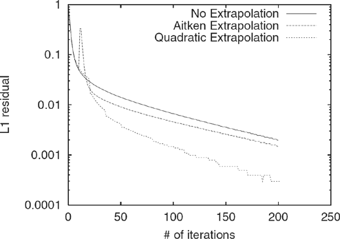
Figure 5.6 Comparison of convergence rates for Power Method, Aitken Extrapolation, and Quadratic Extrapolation on the STANFORD.EDU dataset for c = 0.99. Aitken Extrapolation was applied at the 10th iteration, Quadratic Extrapolation was applied every 15th iteration. Quadratic Extrapolation performs the best by a considerable degree. Aitken suffers from a large spike in the residual when first applied.

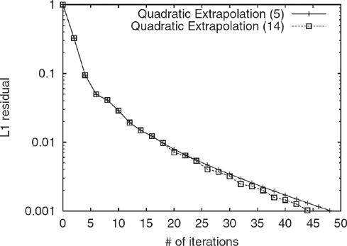
Figure 5.7 Comparison of convergence rates for Quadratic Extrapolation on LARGEWEB for c = 0.95, under two scenarios: Extrapolation was applied the first 5 possible times in one case, and all 14 possible times in the other. Applying it only 5 times achieves nearly the same benefit in this case.

For instance, in Figure 5.7, we plot the convergence when Quadratic Extrapolation is applied 5 times compared with when it is applied as often as possible (in this case, 14 times), to achieve a residual of 0.001. Note that the additional applications of Quadratic Extrapolation do not lead to much further improvement. In fact, once we factor in the 0.5 iteration-cost of each application of Quadratic Extrapolation, the case where it was applied 5 times ends up being faster.

5.3.4 Discussion

Like Aitken and Epsilon Extrapolation, Quadratic Extrapolation makes the assumption that an iterate can be expressed as a linear combination of a subset of the eigenvectors of A in order to find an approximation to the principal eigenvector of A. In Aitken and Epsilon Extrapolation, we assume that can be written as a linear combination of the first two eigenvectors, and in Quadratic Extrapolation, we assume that can be written as a linear combination of the first three eigenvectors. Since the assumption made in Quadratic Extrapolation is closer to reality, the resulting approximations are closer to the true value of the principal eigenvector of A.

While Aitken and Epsilon Extrapolation are logical extensions of existing acceleration algorithms, Quadratic Extrapolation is completely novel. Furthermore, all these algorithms are general purpose. That is, they can be used to compute the principal eigenvector of any large, sparse Markov matrix, not just the Web graph. They should be useful in any situation where the size and sparsity of the matrix is such that a QR factorization is prohibitively expensive.

Both Aitken and Quadratic Extrapolation assume that none of the nonprincipal eigenvalues of the hyperlink matrix are known. However, in the previous chapter, we showed that the modulus of the second eigenvalue of A is given by the damping factor c. Note that the Web graph can have many eigenvalues with modulus c (e.g., one of c, –c, ci, and –ci). In the next sections, we will discuss Power Extrapolation, which exploits known eigenvalues of A to accelerate PageRank.

5.4 POWER EXTRAPOLATION

5.4.1 Simple Power Extrapolation

5.4.1.1 Formulation

As in the previous sections, the simplest extrapolation rule assumes that the iterate can be expressed as a linear combination of the eigenvectors and , where m₂ has eigenvalue c:

Now consider the current iterate ^(k); because the Power Method generates iterates by successive multiplication by A, we can write ^(k) as

Plugging in λ₂ = c, we see that

This allows us to solve for in closed form:

5.4.1.2 Results and Discussion

Figure 5.8 shows the convergence of this simple power extrapolation algorithm (which we shall call Simple Extrapolation) and the standard Power Method, where there was one application of Simple Extrapolation at iteration 3 of the Power Method. Simple Extrapolation is not effective, as the assumption that c is the only eigenvalue of modulus c is inaccurate. In fact, by doubling the error in the eigenspace corresponding to eigenvalue –c, this extrapolation technique slows down the convergence of the Power Method.

5.4.2 A² Extrapolation

5.4.2.1 Formulation

The next extrapolation rule assumes that the iterate ^(k–2) can be expressed as a linear combination of the eigenvectors u₁, u₂, and u₃, where u₂ has eigenvalue c and u₃ has eigenvalue –c:

Figure 5.8 Comparison of convergence rates for Power Method and Simple Extrapolation on LARGEWEB for c = 0.85.

Now consider the current iterate ; because the Power Method generates iterates by successive multiplication by A, we can write as

Plugging in λ₂ = c and λ₃ = –c, we see that

This allows us to solve for in closed form:

A² Extrapolation eliminates error along the eigenspaces corresponding to eigenvalues of c and –c.

5.4.2.2 Results and Discussion

Figure 5.9 shows the convergence of A² extrapolated PageRank and the standard Power Method where A² Extrapolation was applied once at iteration 4. Empirically, A² extrapolation speeds up the convergence of the Power Method by 18%. The initial effect of the application increases the residual, but by correctly subtracting much of the largest non-principal eigenvectors, the convergence upon further iterations of the Power Method is sped up.

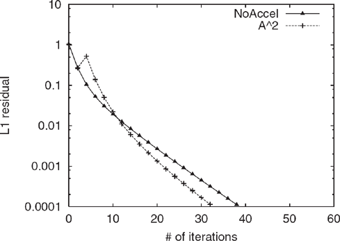
Figure 5.9 Comparison of convergence rates for Power Method and A² Extrapolation on LARGEWEB for c =0.85.

5.4.3A^d Extrapolation

5.4.3.1 Formulation

The previous extrapolation rule made use of the fact that (–c)² = c². We can generalize that derivation to the case where the eigenvalues of modulus c are given by cd_i, where {d_i} are the dth roots of unity. From Theorem 2.1 of [35] and Theorem 1 given in the Appendix, it follows that these eigenvalues arise from leaf nodes in the strongly connected component (SCC) graph of the Web that are cycles of length d. Because we know empirically that the Web has such leaf nodes in the SCC graph, it is likely that eliminating error along the dimensions of eigenvectors corresponding to these eigenvalues will speed up PageRank.

We make the assumption that can be expressed as a linear combination of the eigenvectors {u₁,…, u_d+1}, where the eigenvalues of {u₂, …, u_d+1} are the dth roots of unity, scaled by c:

Then consider the current iterate ^(k); because the Power Method generates iterates by successive multiplication by A, we can write ^(k) as

But since λ_i is cd_i, where d_i is a dth root of unity

Algorithm 8: Power Extrapolation

Algorithm 9: Power Method with Power Extrapolation

This allows us to solve for in closed form:

For instance, for d = 4, the assumption made is that the nonprincipal eigenvalues of modulus c are given by c, –c, ci, and –ci (i.e., the 4th roots of unity). A graph in which the leaf nodes in the SCC graph contain only cycles of length l, where l is any divisor of d = 4 has exactly this property.

Algorithms 8 and 9 show how to use A^d Extrapolation in conjunction with the Power Method. Note that Power Extrapolation with d = 1 is just Simple Extrapolation.

The overhead in performing the extrapolation shown in Algorithm 8 comes from computing the linear combination , an O(n) computation.

In our experimental setup, the overhead of a single application of Power Extrapolation is 1% of the cost of a standard power iteration. Furthermore, Power Extrapolation needs to be applied only once to achieve the full benefit.

5.4.3.2 Results and Discussion

In our experiments, A^d Extrapolation performs the best for d = 6. Figure 5.10 plots the convergence of A^d Extrapolation for d ∈ {1, 2, 4, 6, 8}, as well as of the standard Power Method, for c = 0.85 and c = 0.90.

The wallclock speedups, compared with the standard Power Method, for these 5 values of d for c = 0.85 are given in Table 5.1.

For comparison, Figure 5.11 compares the convergence of the Quadratic Extrapolated PageRank with A⁶ Extrapolated PageRank. Note that the speedup in convergence is similar; however, A⁶ Extrapolation is much simpler to implement, and has negligible overhead, so that its wallclock-speedup is higher. In particular, each application of Quadratic Extrapolation requires about half of the cost of a standard iteration, and must be applied several times to achieve maximum benefit.

Figure 5.10 Convergence rates for A^d Extrapolation, for d ∈ {1, 2, 4, 6, 8}, compared with standard Power Method.

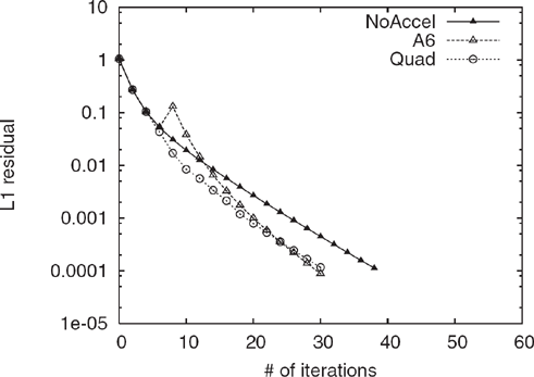
Figure 5.11 Comparison of convergence rates for Power Method, A⁶ Extrapolation, and Quadratic Extrapolation on LARGEWEB for c = 0.85.

Table 5.1 Wallclock speedups for A^d Extrapolation, for d ∈ 1, 2, 4, 6, 8, and Quadratic Extrapolation

Figure 5.12 Comparison of the L₁ residual versus KDist and K_min for PageRank iterates. Note that the two curves nearly perfectly overlap, suggesting that in the case of PageRank, the easily calculated L₁ residual is a good measure for the convergence of query-result rankings.

5.5 MEASURES OF CONVERGENCE

In this section, we present empirical results demonstrating the suitability of the L₁ residual, even in the context of measuring convergence of induced document rankings. In measuring the convergence of the PageRank vector, prior work has usually relied on δ_k = ||Ax^(k) − x^(k)||_p, the L_p norm of the residual vector, for p = 1 or p = 2, as an indicator of convergence [7, 56]. Given the intended application, we might expect that a better measure of convergence is the distance, using an appropriate measure of distance, between the rank orders for query results induced by Ax^(k) and x^(k). We use two measures of distance for rank orders, both based on the the Kendall’s rank correlation measure [47]: the KDist measure, defined below, and the K_min measure, introduced by Fagin et al. in [27]. To determine whether the residual is a “good” measure of convergence, we compared it to the KDist and K_min of rankings generated by Ax^(k) and x^(k).

We show empirically that in the case of PageRank computations, the L₁ residual δ_k is closely correlated with the KDist and K_min distances between query results generated using the values in Ax^(k) and x^(k).

We define the distance measure, KDist as follows. Consider two partially ordered lists of URLs, τ₁ and τ₂, each of length k. Let U be the union of the URLs in τ₁ and τ₂. If ρ₁ is U − τ₁, then let τ′₁ be the extension of τ₁, where τ′₁ contains ρ₁ appearing after all the URLs in τ₁³. We extend τ₂ analogously to yield τ′₂. KDist is then defined as

In other words, KDist (τ₁, τ₂) is the probability that τ′₁ and τ′₂ disagree⁴ on the relative ordering of a randomly selected pair of distinct nodes (u, v) ∈ U × U.

To measure the convergence of PageRank iterations in terms of induced rank orders, we measured the KDist distance between the induced rankings for the top 100 results, averaged across 27 test queries, using successive power iterates for the LARGEWEB dataset, with the damping factor c set to 0.9.⁵ The average residuals using the KDist, K_min, and L1 measures are plotted in Figure 5.12.⁶ Surprisingly, the L₁ residual is almost perfectly correlated with KDist, and is closely correlated with K_min.⁷ A rigorous explanation for the close match between the L₁ residual and the Kendall’s τ-based residuals is an interesting avenue of future investigation.