10 Modeling Variance

This chapter addresses models that incorporate more than one kind of variability, variously called mixed, multilevel, multistratum, or hierarchical models. It starts by considering data with (1) changing amounts of variability or (2) correlation among data points. These kinds of data can be modeled adequately with the tools introduced in previous chapters. The last part of the chapter considers data with two or more qualitatively different sources of variability. These kinds of data are much more challenging to model, but they can be fitted with analytical or numerical integration techniques or via MCMC. This chapter is more conceptual and less technical than previous chapters.

10.1 Introduction

Throughout this book we have partitioned ecological models into deterministic (Chapter 3) and stochastic (Chapter 4) submodels. For example, we might use a deterministic logistic function to describe changes in mean population density with increasing rainfall and a Gamma stochastic distribution to describe the natural variation in population density at a particular level of rainfall. We have focused most of our attention on constructing the deterministic model and testing for differences in parameters among groups or as a function of covariates. For the stochastic model, we have stuck to fitting single parameters such as the variance (for normally distributed data) or the overdispersion parameter (for negative binomially distributed data) to describe the variability around the deterministic expectation. We have assumed that the variance parameter is constant within groups, and that we can use a single distribution to describe the variability.

This chapter will explore more sophisticated stochastic models for ecological data. Section 10.2 is a warmup, presenting models where the variance may differ among groups or change as a function of a covariate. These models are easy to fit with our existing tools. Section 10.3 briefly reviews models for correlation among observations, useful for incorporating spatial and temporal structure.

Sections 10.4 and 10.5 tackle models that incorporate more than one type of variability, referred to as mixed, multilevel, multistratum, or hierarchical models.

Section 10.4 discusses how to use canned procedures in R to fit multilevel models— or to cheat and avoid fitting multilevel models at all—while Section 10.5 briefly describes strategies for tackling more general multilevel models.

The most common multilevel models are block models, which divide observations into discrete groups according to their spatial or temporal locations, genetic identity, or other characteristics. The model assigns each block a different random mean, typically drawn from a normal or log-normal distribution. Individual responses within blocks vary around the block mean, most frequently according to a normal distribution but sometimes according to a Poisson or binomial sampling distribution. In survival analysis, block models are called shared frailty models (Therneau et al., 2003).

Individual-level models allow for variation at the individual rather than the group level. When individuals are measured more than once, the resulting repeated-measures models can be analyzed in the same way as block models. They may also allow for temporal correlation among measurements, and more sophisticated versions can quantify random variation among individuals in the parameters of nonlinear models (Vigliola et al., 2007).

When individuals are measured only once, we lose most of our power to discriminate among-individual and within-individual variation. We can still make progress, however, if we assume that the observed variation in individual responses is a combination of among-individual variation in a mean response and a random sampling process (either in the ecological process itself, or in our measurement of it) that leads to variation around the mean. The combination of among-individual and sampling variation results in a marginal distribution (the distribution of observations, including both levels of variability) that is overdispersed, or more variable than expected from the sampling process alone.

Finally, when individuals or populations are measured over time we have to distinguish between measurement and process error, because these two sorts of variability act differently on ecological dynamics. Process error feeds back to affect the ecological system in the next time step, while measurement error doesn't. We defer analysis of such dynamical models to Chapter 11.

Building models that combine several deterministic processes is straightforward. For example, if we know the functions for mean plant biomass as a function of light availability (say B(L) = aL/(b + L)) and for mean fecundity as a function of biomass (say F(B) = cB^d), we can easily combine them mathematically in order to use the combined function in a maximum likelihood estimate (F(L) = c(aL/(b + L))^d).^* Incorporating multiple levels of variability in a model is harder because we usually have to compute an integral in order to average over all the different ways that different sources might combine to produce a particular observation. For example, suppose that the probability that a plant establishes in an environment with light availability L is P_L(L) dL (where P_L is the probability density) and the probability that it will grow to biomass B at light level L is P_BL(B|L) dB. Then the marginal probability density P_B(B) that a randomly chosen plant will have biomass B is the combination of all the different probabilities of achieving biomass B at different light levels: ∫P_BL(B|L)P_L(L) dL.

Computing these integrals analytically is often impossible, but for some models the answer is known (Section 10.5.1). Otherwise, we can either use numerical brute force to compute them (Section 10.5.2) or use Markov chain Monte Carlo to compute a stochastic approximation to the integral (Section 10.5.3). These methods are challenging enough that, in contrast to the models of previous chapters, you will often be better off finding an existing procedure that matches the characteristics of your data rather than coding the model from scratch.

10.2 Changing Variance within Blocks

Once we've thought of it, it's simple to incorporate within-block changes in variance into an ecological model. All we have to do is define a sensible model that describes how a variance parameter changes as a function of predictor variables. For example, Figure 10.1 shows data on glacier lilies (Erythronium glandiflorum) that display the typical triangular, or “factor-ceiling,” profile of many ecological data sets (Thomson et al., 1996). The triangular distribution is often caused by an environmental variable that sets an upper limit on an ecological response rather than determining its precise value. In this case, the density of adult flowers (or something associated with adult density) appears to set an upper limit on the density of seedlings, but the number of seedlings varies widely below the upper limit. I fitted the model

where S is the observed number of seedlings and f is the number of flowers. The mean μ is constant, but the overdispersion parameter k increases (and thus the variance decreases) as the number of flowers increases. The R negative log-likelihood function for this model is

Alternatively, the mle2 formula would be

This function resembles our previous examples, except that the variance parameter rather than the mean parameter changes with the predictor variable (f or flowers). Figure 10.1 shows the estimated mean (which is constant) and the estimated upper 90%, 95%, and 97.5% quantiles, which look like stair-steps because the negative binomial distribution is discrete. It also shows a nonparametric density estimate for the mean and quantiles as a function of the number of flowers, as a cross-check of the appropriateness of the parametric negative binomial model. The patterns agree qualitatively—both models predict a roughly constant mean and decreasing upper quantiles. Testing combinations of models that allow mean, variance, both, or neither to vary with the numbers of flowers suggests that the best model is the constant model, but the model fitted here (constant mean, varying k) is the second best, better than allowing the mean to decrease while holding k constant. Thomson et al. (1996) suggested a pattern where the ceiling actually increases initially at small numbers of flowers, but this pattern is hard to establish definitively.

Figure 10.1 Lily data from Thomson et al. (1996); jittered numbers of seedlings as a function of number of flowers. Black lines show fit of a negative binomial model with constant mean and increasing k/decreasing variance; gray lines are from a nonparametric density estimate.

The same general strategy applies for the variance parameter of other distributions such as the variance of a normal distribution or log-normal distribution, the shape parameter of the Gamma distribution, or the overdispersion parameter of the beta-binomial distribution. Just as with deterministic models for the mean value, the variance might differ among different groups or treatment levels (represented as factors in R), might change as a function of a continuous covariate as in the example above, or might depend on the interactions of factors and covariates (i.e., different dependence of variance on the covariate in different groups). Just the variance, or both the mean and the variance, could differ among groups. Use your imagination and your biological intuition to decide on a set of candidate models, and then use the LRT or AIC values to choose among them.

Variance parameters are best fit on the log scale (logσ², logk etc.) to make sure the variances are always positive. For fitting to continuous covariates, use nonnegative functions such as the exponential(σ² = ae^bx) or power (σ² = ax^b), for the same reason.

When using a normal distribution to model the variability is reasonable, you can use the built-in functions gls andgnls from the nlme package: gls fits linear and gnls fits nonlinear models. These models are called generalized (non)linear least squares models.^* The weights argument allows a variety of relationships (exponential, power, etc.) between covariates and the variance. For example, using the fir data, suppose we wanted to fit a power-law model for the mean number of cones as a function of DBH and include a power-law model for the variance as a function of DBH:

Fitting the model with gnls:

The syntax of weights argument is a bit tricky: Pinheiro and Bates (2000) is essential background reading.

10.3 Correlations: Time-Series and Spatial Data

Up to now we have assumed that the observations in a data set are all independent. When this is true, the likelihood of the entire data set is the product of the likelihoods of each observation, and the negative log-likelihood is the sum of the negative log-likelihoods of each observation. Every negative log-likelihood function we have written has contained code like -sum(ddistrib(…,log=TRUE)),either explicitly or implicitly, to capitalize on this fact. With a bit more effort, however, we can write and numerically optimize likelihood functions that allow for correlations among observations.

It's best to avoid correlation entirely by designing your observations or experiments appropriately. Correlation among data points is a headache to model, and it always reduces the total amount of information in the data: correlation means that data points are more similar to each other than expected by chance, so the total amount of information in the data is smaller than if the data were independent. However, if you are stuck with correlated data—for example, because your samples come from a spatial array or a time series—all is not lost. Moreover, sometimes the correlation in the data is biologically interesting: for example, the range of spatial correlation might indicate the spatial scale over which populations interact.

The standard approach to correlated data is to specify a likelihood of correlated data, usually using a multivariate normal distribution. The probability distribution of the multivariate normal distribution (dmvnorm in the emdbook package) is

where x is a vector of data values, μ is a vector of means, and V is the variance-covariance matrix (|V| is the determinant of V—see below—and ^T stands for transposition). The formula looks scary, but like most matrix equations you can understand it by making analogies to the scalar (i.e., nonmatrix) equivalent, in this case the univariate normal distribution

The term exp (–(x–μ)^TV^–1(x–μ)) is the most important part of the formula, equivalent to the exp (– (x–μ²/(2σ²)) term in the univariate normal distribution. (x–μ) is the deviation of the observations from their theoretical mean values. Multiplying by V^–1 is equivalent to dividing by the variance, and multiplying by (x–μ)^T is equivalent to squaring the deviations from the mean. The stuff in front of this term is the normalization constant. The |V| matches the σ² in the normalization constant of the univariate normal, and the √2π term is raised to the nth power to normalize the n-dimensional probability distribution.

If all the points are actually independent and have identical variances, then the variance-covariance matrix is a diagonal matrix with σ² on the diagonal:

Comparing (10.3.1) and (10.3.2) one term at a time shows that the multivariate normal reduces to a product of identical univariate normal probabilities in this case. For a diagonal matrix with σ² on the diagonal, the inverse is a diagonal matrix with 1/σ² on the diagonal, so the matrix multiplication(x –μ)^TV^–1(x–μ) works out to ∑_i(x_i –μ_i) ²/σ²—the sum of squared deviations. Exponentiating this sum gives a product. For a diagonal matrix, the determinant |V| is the product of the diagonal elements, so for the identical-variance case |V| = (σ²)ⁿ, which is proportional to the product of the normalizing constants for n independent normal distributions.

If the points are independent but each point has a different variance—like assigning different variances to different groups with one individual in each group—then

Carrying through the exercise of the previous paragraph will show that the multivariate normal reduces to a product of univariate normals, each with its own variance.

The exponent term is now half the weighted sum of squares Σ(x_i — μ_i)²/σ_i² with the deviation for each point weighted by its own variance; data points with larger variances have less influence on the total.

Most generally,

The off-diagonal elements σ_ij quantify the covariance between points i and j. We could also specify this information in terms of the correlation matrix C = {ρ_ij} ={ρ_ij/√σ_i²σ_j²}. The diagonal elements of the correlation matrix ρ_ii all equal 1, and the off-diagonal elements range between —1 (perfect anticorrelation) and 1 (perfect correlation). The variance-covariance matrix V must be symmetric (i.e., σ_ij = σ_ji). In this case there is no way to express the exponent as a sum of independent normals, but its meaning is the same as in the previous cases: it weights combinations of deviations by the appropriate variances and covariances.

To fit a correlated multivariate normal model, you would need to specify parameters for the variance-covariance matrix V. In principle you could specify n(n + 1)/2 different parameters for each of the distinct entries in the matrix (since the matrix is symmetric there are n(n + 1)/2 rather than n² distinct entries), but there are two reasons not to. First, such a general parameterization takes lots of parameters. Unless we have lots of data, we probably can't afford to use up so many parameters specifying the variance-covariance matrix. Second, in addition to being symmetric, variance-covariance matrices must also be positive definite, which means essentially that the relationships among points must be consistent.^* For example,

is not a valid correlation matrix, even though it is symmetric.^† It states that site 1 is strongly positively correlated with site 2 (ρ₁₂ = 0.9), and site 2 is strongly correlated with site 3 (σ₂₃ = 0.9), but site 1 is strongly negatively correlated with site 3 (σ₁₃ = —0.9), which is not possible.

For these two reasons, modelers usually select from established correlation models that (1) use a small number of parameters to construct a full variance-covariance (correlation) matrix and (2) ensure positive definiteness. For example,

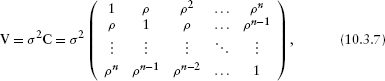
with |ρ | < 1, specifies a correlation matrix C corresponding to sites arranged in a line—or data taken in a temporal sequence—where correlation falls off with the number of steps between sites (sampling times): nearest neighbors (sites 1 and 2, 2 and 3, etc.) have correlation ρ, next-nearest neighbors have correlation ρ², and so forth.^* Other correlation models allow correlation ρ_ij to drop to zero at some threshold distance, or to be a more general function of the spatial distance between sites.

Three different areas of classical statistics use multivariate normal distributions to describe correlation among observations. Repeated-measures ANOVA is a form of analysis of variance that allows the errors to be nonindependent in some way, particularly by building in individual-level variation (see Section 10.4.1) but also by allowing for correlation between successive points in time. Time-series models (Chatfield, 1975; Diggle, 1990; Venables and Ripley, 2002) and spatial models (Ripley, 1981; Cressie, 1991; Kitanidis, 1997; Venables and Ripley, 2002; Haining, 2003) specify correlation structures that make sense in temporal and spatial contexts, respectively.

Generalized least-squares (g[n]ls) allows for correlation among observations, using the correlation argument. These functions include a variety of standard models for temporal and spatial autocorrelation; see ?corClasses (in the nlme package) and Pinheiro and Bates (2000) for more details. The lme and nlme functions, which fit repeated-measures models, also have a correlation argument. The ts package implements time-series models, which incorporate correlation, although the description and methods used are different from the more general models described here. The spatial package will fit trend lines and surfaces with spatial correlation between points.

To construct variance-covariance functions to use in your own custom-made likelihood functions, start with the matrix function (for general matrices) or diag (for diagonal matrices) and extend them. For example, diag(4) produces a 4 × 4 identity matrix (with 1 on the diagonal); diag(c(2,3,4)) produces a 3 × 3 diagonal matrix with variances of 2, 3, and 4 on the diagonal. The row and col functions, which return matrices encoding row and column numbers, are also useful. For example, d=abs(row(M)-col(M))produces a absolute-value distance matrix {|i–j|} with the same dimensions as M, and rho^d produces correlation matrix (10.3.7). The slightly tricky code ifelse(d==0,1,ifelse(d==1,rho,0)) produces a matrix with 1 on the diagonal, rho on the first off-diagonal, and 0 elsewhere, corresponding to correlation only among nearest-neighbor sites.

If your data are irregularly spaced or two-dimensional, you can start by computing a matrix of the distances between points, using d=as.matrix(dist(cbind (x,y))).^† Then you can easily use the distance matrix to compute exponential (proportional to e^–d), Gaussian (proportional to e^–d2), or other spatial correlation matrices. Consult Venables and Ripley (2002) or a spatial statistics reference for more details.

Once you have constructed a correlation matrix, multiply it by the variance to get a covariance matrix suitable for use with the dmvnorm density function, for example, negative log-likelihood

where z is a vector of data, mu is a mean vector, and V is one of the variance-covariance matrices defined above. You can use the mvrnorm command from the MASS package to generate random, correlated normal deviates. For example, mvrnorm(n=1,mu=rep(3,5),Sigma=V) produces a five-element vector with a mean of 3 for each element and variance-covariance matrix V. Asking mvrnorm for more than one random deviate (n > 1) will produce a five-column matrix where each row is a separate draw from the multivariate distribution.

Statisticians usually deal with correlated data that is nonnormal (e.g., Poisson or binomial) by combining a multivariate normal model for the underlying mean values with a nonnormal distribution based on these varying means. We usually exponentiate the MVN distribution to get a multivariate lognormal distribution so that the means are always positive. For example, to model correlated Poisson data we could assume that A, the vector of expected numbers of counts at each point, is the exponential of a multivariate normally distributed variable:

Here Y is a vector of counts at different locations; Λ (a random variable) is a vector of expected numbers of counts (intensities); μ is a vector of the logs of the average intensities; and V describes the variance and correlation of intensities. If we had already used one of the recipes above to construct a variance-covariance matrix V, and had a model for the mean vector mu, we could simulate the values as follows:

Unfortunately, even though we can easily simulate values from this distribution, writing down a likelihood for this model is difficult because there are two different levels of variation. The rest of the chapter discusses how to formulate and estimate the parameters for such multilevel models.

10.4 Multilevel Models: Special Cases

While correlation models assume that samples depend on each other as a function of spatial or temporal distance, with overlapping neighborhoods in space or time, traditional multilevel models usually break the population into discrete groups such as family, block, or site. Within groups, all samples are equally correlated with each other. If samples 1 and 2 are from one site and samples 3 and 4 are from another, each pair would be correlated and we would write down this variance-covariance matrix:

Equivalently, we could specify a random-effects model that gives each group its own random offset from the overall mean value. The correlation model (10.4.1) is formally identical to a random-effects model where the value of the jth individual in the ith group is

where ε_i ~ N(0, σ_b²) is the level of the random effect in the ithblock and ε_ij ~ N(0, σ_w²) is the difference of the jth individual in the ith block from the block mean. The among-group variance σ_b² and within-group variance ε_w² correspond to the correlation parameters (ρ,σ²):

Classical models usually describe variability in terms of random effects because constructing huge variance-covariance matrices is very inefficient.

10.4.1 Fitting (Normal) Mixed Models in R

Some special kinds of block models can be fitted with existing tools in R and in many other statistics packages. Models with two levels of normally distributed variation are called mixed-effect models (or just mixed models) because they contain a mixture of random (between-group) and fixed effects. Classical block ANOVA models such as split-plot and nested block models fall into this category (Quinn and Keogh, 2002; Gotelli and Ellison, 2004). If the variation in your model is normally distributed, your predictors are all categorical, and your design is balanced, you can use the aov function with an Error term to fit mixed models (Venables and Ripley, 2002). The nlme package, and the newer, more powerful (but poorly documented) lme4 package fit a far wider range of mixed models (Pinheiro and Bates, 2000; Gelman and Hill, 2006). These packages allow for unbalanced data sets as well as random effects on parameters (e.g., ANCOVA with randomly varying slopes among groups), and nonlinear mixed-effect models (e.g., an exponential, power-law, logistic, or other nonlinear curve with random variation in one or more of the parameters among groups).

10.4.2 Generalized Linear Mixed Models

Generalized linear mixed models, or GLMMs, are a cross between mixed models and generalized linear models (p. 308). GLMMs combine link functions and exponential-family variation with random effects. The random effects must be normally distributed on the scale of the linear predictor—meaning on the scale of the data as transformed by the link function. For example, for a Poisson model with a log link, the between-group variation would be log-normal. GLMMs are cutting edge, and the methods for solving them are evolving rapidly. The glmmPQL function in the MASS package can fit an approximation to GLMMs, but one that is sometimes inaccurate (Breslow and Clayton, 1993; Breslow, 2003; Jang and Lim, 2005). The glmmML and lme4 packages offer more robust GLMM fitting algorithms; so does J. Lindsey's repeated package, documented in his book (Lindsey, 1999) and available on his Web page (linked under “Related Projects” on the R project page). If you want to be thorough, it may also be worth cross-checking your results with PROC GLIMMIX or NLMIXED in SAS.

R has built-in capabilities for incorporating random effects into a few other kinds of models. Generalized additive mixed models (GAMMs) (gamm in the mgcv package) allow random effects and exponential-family variation with models where spline curves make up the deterministic part of the model. Frailty models (frailty in the survival package) incorporate Gamma, t, or normally distributed variation among groups in a survival analysis. Some other variations such as nonnormal repeated-measures models are described by Lindsey (1999a, 2001, 2004).

10.4.3 Avoiding Mixed Models

Even when canned packages are available, fitting mixed models can be difficult. The algorithms do not always converge, especially when the number of groups is small. If your design is linear, balanced, and has only nested random effects, then aov should always work, but otherwise you may be at a loss.

If you want to avoid fitting mixed models altogether, one option is to fit fixed-effect models instead, estimating a parameter for each group rather than a random variable for the among-group variation (Clark et al., 2005). You will probably lose some power this way, so the results are likely to be conservative.^* As a second option, Gotelli and Ellison (2004, p. 182) suggest that when you have a simple nested design (i.e., subsamples within blocks) you should often just collapse each group's data by computing its mean and do a single-level analysis. This will be disappointing if you were hoping to glean information about the within-group variance, but it is simple and in many cases will give the same p-value as the classical algorithm coded by aov. Finally, you can try to convince yourself (and your reviewers, readers, or supervisor) that between-group variation is unimportant by fitting the model ignoring blocks and then examining the variation of the residuals between blocks both graphically and statistically. To justify ignoring between-group variation in the model, you must show that the between-group variation in the residuals is both statistically and biologically irrelevant. Biologically relevant variation is an important warning sign even if it is not statistically significant.

10.5 General Multilevel Models

Now suppose that your data do not allow analysis by classical tools and that you are both brave and committed to finding out what a multilevel model can tell you.

10.5.1 Analytical Models for Marginal Distributions

In some cases, it may be possible to solve the integrals that arise in multilevel problems analytically. In this case you can fit the marginal distribution directly to your data. The marginal distribution describes the combination of multiple stochastic processes but doesn't attempt to provide information about the individual processes—analogous to knowing the row and column sums (the marginal totals) of a table without knowing the distribution of values within the table.

If you're comfortable with math, you can read an advanced treatment such as Bailey (1964) or Pielou (1977) to learn how to solve these problems. Otherwise, you should do some research to see if someone has already found the answer for your model. The most common of these distributions—the negative binomial arising from a Poisson sampling process with underlying Gamma-distributed variability, the beta-binomial arising from binomial sampling with underlying Beta-distributed variability, and the Student t distribution arising from normally distributed variation with Gamma-distributed variability in the inverse variance—were already discussed on p. 140. Zero-inflated distributions (p. 139) are another example of a multilevel process—the combination of a presence/absence process and a discrete sampling process—for which it is fairly easy to figure out the marginal distribution.

If your multilevel process involves summing several values—for example, if the measured value is the sum of a normally distributed block mean and a normally distributed individual variation—then the marginal distribution is called a convolution. If X and Y are random variables with probability densities P_X and P_Y, then the probability density of X + Y is

The intuition behind this equation is that we are adding up all the possible ways we could have gotten z. If X = x, then the value of Y must be z–x in order for X + Y to equal z, so we can calculate the total probability by integrating over all values of x. The convolutions of distributions with themselves—i.e., the distribution of sums of like variables—can sometimes be solved analytically. The sum of two normal variables N(μ₁, σ₁²) and N(μ₂, σ₂²) is also normal (N(μ₁ + μ₂,σ₁² + σ₂²)); the sum of two Poisson variables is also Poisson (Pois(λ₁) + Pois(λ₂) ~ Pois(λ₁ + λ₂)); and the sum of n exponential variables with the same mean is Gamma distributed with shape parameter n. These solutions are simple, but they also warn us that we may sometimes face an identifiability problem (p. 333) when we try to separate multiple levels of variability. If we know only that the sum of two normally distributed variables is N(μ,σ²), then we can't recover any more information about the means and variance of the individual variables—except that the variances are between 0 and σ². (In the case of classical block models we also know which group any individual belongs to, so we can partition variability within and among groups.)

10.5.2 Numerical Integration

If you can't find anyone who has computed the marginal distribution for your problem analytically, you may still be able to compute it numerically.

A common problem in forest ecology is estimating the distribution of growth rates g_i of individual trees in a stand from size measurements S_i in successive censuses: g_i = S_i,2–S_i,1. Foresters commonly assume that adult trees can't shrink, or at least not much, but it's typical to observe a small proportion of individuals in a data set whose measured size in the second census is smaller than their initial size. If we really think that measurement error is negligible, then we're forced to conclude that the trees actually shrank. It's standard practice to go through the data set and throw out negative growth values, along with any that are unrealistically big. Can we do better?

Although it is sensible to throw out really extreme values, which may represent transcription errors (being careful to keep the original data set intact and document the rules for discarding outliers), we may be able to extract information from the data set both about the “true” distribution of growth rates and about the distribution of errors. The key is that the distributions of growth and error are assumed to be different. The error distribution is symmetric and narrowly distributed (we hope) around zero, while the growth distribution is positive and right-skewed. Thus the negative tail of the distribution tells us about error—negative values must contain at least some error.

Specifically, let's assume a Gamma distribution of growth (we could equally well use a lognormal) and a normal distribution of error. The growth distribution has parameters a (shape) and s (scale), while the error distribution has just a variance σ²—we assume that errors are equally likely to be positive or negative, so the mean is zero. Then

For normally distributed errors, we can also express this as the sum of the true value and an error term:

According to the convolution formula, the likelihood of a particular observed value is

The log-likelihood for the whole data set is

TABLE 10.1
Results of convolution analysis of tree growth

Unfortunately we can't interchange the logarithm and the integral, which would make everything much simpler.

We can easily simulate some fake “data” from this system with plausible parameters in order to test our approach:

In the R supplement (Section 10.8), I defined a getdist function that implements (10.5.2)-(10.5.5). I then used mle2 and confint to find the maximum likelihood values and profile confidence limits (Table 10.1). It was slow, though: it took about 3 minutes (for a total of 137 function evaluations) to find the MLE using Nelder-Mead and 164 minutes to calculate the profile confidence intervals. The estimates are encouragingly close to the true values, and the confidence limits are reasonable. The quadratic confidence intervals, while too narrow for σ, are close enough to the profile confidence intervals that the extra 2.5 hours of computation may have been unnecessary. Figure 10.2 plots the observed histogram along with the estimated and true distributions of actual growth rates and the estimated and true distributions of measurement error. Excitingly, we can actually recover accurate information about the growth rates and the measurement process in this example.

Numerical integration works well here, although it's slow if we insist on calculating profile confidence limits. Hand-coded numerical integration in R will always be slower, and less stable, than the special-case algorithms built into packages like lme4 or glmmML. A commercial package called AD Model Builder uses sophisticated integration techniques to solve some very difficult multilevel modeling problems, but I have not evaluated it (Kitakado et al., 2006; Skaug and Fournier, 2006). Gelman and Hill (2006) primarily use R and BUGS to fit multilevel models, but they provide an appendix that describes how to fit some multilevel models in SAS, AD Model Builder, and other packages. Brute-force numerical integration can work reasonably well as long as you have enough data (both enough individual data points and enough groups) and as long as your problem has only one, or at most two, random variables to integrate. The estimation process is fairly straightforward, and numerical failures are usually obvious—although you should do all the usual checks for convergence.

10.5.3 MCMC for Mixed Models

Most of the time, brute-force numerical integration as illustrated above is just too hard. Once you have to integrate over more than one or two random variables, computing the integrals becomes extremely slow. MCMC is an alternative way of doing these high-dimensional integrals, and it gets you confidence limits “for free.” The disadvantages are that (1) it may be slower than sufficiently clever numerical integration approximations; (2) you have to deal with the Bayesian framework, including deciding on a set of reasonable priors (although Lele et al. (2007) recently suggested a simple method for using MCMC to do ML estimation for multilevel models); and (3) in badly determined cases where your model is poorly defined or where the data don't really contain enough information, BUGS may give you an answer that doesn't make sense instead of just crashing—which is really bad.

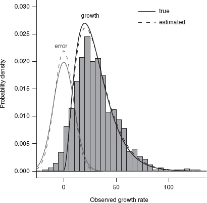
Figure 10.2 True and estimated distributions of growth rates and measurement error for simulated forest data. Histogram, observed data. Lines, true and estimated distributions of actual growth rate and measurement error.

The BUGS input file for the Gamma-normal model is extremely simple:

The first half of the model statement is a direct translation of the model (10.5.2): for each value in the data set, the observed value is assumed to be drawn from a normal distribution centered on the true value, which is in turn drawn from a Gamma distribution.

The second half of the model statement specifies vague Gamma-distributed priors. As mentioned in Chapter 7, BUGS uses slightly different parameterizations from R for the normal and Gamma distributions. It specifies the normal by the mean and the precision τ , which is the reciprocal of the variance, and the Gamma by the shape parameter (just as in R) and the rate parameter, which is the reciprocal of the scale parameter. The mean of the gamma distribution is shape/rate and the variance is shape/rate²; thus a standard weak Gamma prior uses equal shape and rate parameters (i.e., a mean of 1), with both the shape and the rate parameter small (i.e., a large variance). In this case I've chosen (0.01, 0.01) (but see Gelman (2006) for possible problems with this choice).

We'd like to run chains starting from overdispersed starting points, as recommended in Chapter 7, so that we can run a Gelman-Rubin diagnostic test to see if the chains have converged. However, it's still very important to start with sensible starting values (so that BUGS doesn't crash or take forever to burn in). A good strategy is to find a reasonable starting point and then change different parameters by up to an order of magnitude to get overdispersed starting points.

We can estimate a starting point for the Gamma parameters by fitting a Gamma distribution just to the nonzero observations:

We can estimate a starting value for the precision (τ) by selecting the negative observations, replicating them with the opposite sign, and calculating the reciprocal of the variance:

You're not required to specify starting values for all of the parameters—if you don't, BUGS will pick a random starting value from the prior distribution for that parameter. However, BUGS will often crash or converge slowly with random starting values, especially if you use very weak priors. We will start the chains for the true growth rates from 1 or from the observed growth rate for each individual, whichever is greater; this strategy avoids negative values for the true growth rate, which are impossible according to our model.

We specify a list of initial values for each chain; in this case I've decided to start one chain at the values of the crude estimates calculated above, and the other chains with perturbations of those estimates, with one or the other of the parameters halved or increased to 150%. I didn't bother to perturb the starting values for the rate, but you could in a more thorough analysis.

We need to specify the data for BUGS:

Finally, we specify for which parameters of the model we want BUGS to save information. Of course we want to track the parameters of our model. In addition, it will be interesting to see what BUGS estimates for the true values, uncorrupted by measurement error, of both the minimum observed value in the data set (which obviously contains a lot of measurement error, since its value is -15.7) and one of the values closest to the median.^*

Running the model:

BUGS took 264 minutes to run the models. The Gelman-Rubin statistics were all well below the rule-of-thumb cutoff of 1.2, suggesting that the chains had converged. Using as.mcmc to convert the BUGS result gnl.bugs to a coda object and running traceplot and densityplot confirmed graphically that the chains gave similar answers (Table 10.2), and that the posterior distributions are approximately normal: the Gelman-Rubin test makes this assumption, so it's good to check. While the estimated “true” value of the median point is close to its observed value of 28.2, the Bayesian model correctly adjusted the estimated true value for the minimum point from its observed value (– 15.7) to a small but definitely positive value. The estimates of the values of particular data points have wide distributions—it would be too good to be true if we could use MCMC to magically get rid of observation error.

TABLE 10.2
Results of WinBUGS run on Gamma-normal model

10.6 Challenges

Multilevel models are hard to implement. General linear models like linear regression represent one extreme, where you can put in any kind of data and know that you will get a rapid, technically correct (if not necessarily sensible) answer. Multilevel models represent the other extreme: the methods for fitting them are computationally demanding and must be carefully tuned to a particular type of problem to ensure an efficient and correct solution. As with analytical solutions, if you are not ready for a technical challenge, your best bet is to find a prebuilt solution for your class of models. Another issue we have to face as we incorporate more levels of variability is identifiability. Unidentifiable parameters are those that are impossible to estimate separately from our data. For example, if we tried to estimate a linear model with two different intercepts (Y = a₁ + a₂ + bX), instead of the more sensible Y = a + bX, any answer where a₁ + a₂ = a would fit equally well. We would have the same problem with the coefficients of two predictor variables that were perfectly correlated. Similarly, there is no way to identify catchability—the probability that you will observe an individual—from a single observational sample; you simply don't have the information to estimate how many animals or plants you failed to count. Most of these cases of “perfect” unidentifiability are easily detectable by common sense, although they can be obscured by complex models. Always remember that there is no free lunch: if a procedure for estimating parameters seems too good to be true, be suspicious.

Weak identifiability is more common than perfect unidentifiability. Weakly identifiable parameters are hard to estimate even with large, clean data sets—and practically impossible to estimate with moderate-size noisy data sets. Identifiability problems are not limited to multilevel models, but they are particularly common there. Weak identifiability is related to a lack of statistical power; it means that your model is structured in such a way that an enormous amount of data or very extreme kinds of data are needed in order to have the power to differentiate ecological processes.

The best outcome of analyzing an unidentifiable or weakly identifiable model is for your estimation procedure to crash: at least you will know something is wrong. The worst outcome is for your estimation procedure to give you a wrong answer, or one that depends in a sensitive way on the details of your numerical algorithm or your prior. Weak identifiability in MLE analysis leads either to numerical problems or to apparently well-defined, but misleadingly precise, answers; weak identifiability in MCMC analyses leads to poor convergence. In the worst case, chains may move through parameter space so slowly that it's hard to see that they are not converging. The best defenses against identifiability problems are (1) care and common sense in defining models (always remember the “no free lunch” principle); (2) examining model diagnostics—confidence intervals, convergence statistics; and the difference between prior and posterior distributions; and (3) running models with known inputs (i.e., simulations), with different amounts of data and different amounts of noise, to see when they are actually capable of getting the right answers.

Coming to grips with the difficulty of separating different types of variability, like coming to grips with limitations on statistical power (Chapter 5), can be sobering. Schnute (1994) says in a paper on state-space models (one kind of multilevel model) that

the outcome of the analysis often depends critically on the values of [many variance] parameters, and it is generally impossible to estimate all of them…Statistically, the likelihood surface [may be] “flat”, i.e. insensitive to large parameter changes. In cases like this, a large number of conflicting scenarios appear equally consistent with the known data, and the analyst has no objective means to choose among them.

This apparent limitation can be turned into an advantage…State-space model design forces essential questions to be asked about underlying processes, observed data, and sources of variability. When these questions are answered honestly, the model may point to scenarios consistent with the data but in conflict with the prevailing view. If so, the modeling effort can help to delineate the limits of current knowledge and to establish rational priorities for future data collection.

Put another way, acknowledging the many different types of uncertainty that actually exist in our models may make us realize that we know less than we thought we did about the possible dynamics of our study system, and may drive us to make more observations, or more useful kinds of observations.

10.7 Conclusion

Why then are multilevel models worth so much effort?

They are clearly the wave of the future in ecological statistics. Books like Gelman and Hill (2006) and Clark (2007), along with a rapidly growing collection of papers in ecology and statistical ecology, demonstrate these models' potential for understanding ecological processes. We know that ecological systems are variable at every level, and multilevel models give us a framework for estimating this variability at multiple levels rather than lumping it into a single error term. Our statistical models should match our conceptual models as closely as possible. If we are interested in the differences among individuals or sites or genotypes, we would often be satisfied with knowing the amount of variability among groups rather than trying to estimate a value for every individual.

Furthermore, estimating the variability in this way may be more parsimonious than estimating fixed effects for every individual or group. While fixed effects require an additional parameter for every additional group in the model, estimating variability takes only a single parameter (the variance) no matter how many groups there are (Kenward and Roger, 1997).^*

Although multilevel models are hard to implement and computationally challenging, things are getting better. Computers are faster every year, and infrastructure like grid computing is making it easier to access computing power beyond your desktop (Wang et al., 2005). Tools for Bayesian and maximum likelihood estimation are constantly improving, both in the power and breadth of algorithms available and in the convenience, interoperability, and robustness of software (Kerman and Gelman, 2006; Skaug and Fournier, 2006).

Multilevel models are data-hungry. If you are a typical ecological experimenter with a small, noisy data set, you may not be able to apply multilevel models to your data set (Clark et al., 2005), although Bayesian methods can help if you are willing to specify informative priors. On the other hand, if you have a large, but very noisy, data set, then multilevel models may be the perfect tool. Because of data collection tools such as data loggers, remote sensing, radiotelemetry, and climate proxies, and data synthesis tools such as Web databases, meta-analysis, and citizen science initiatives, more and more ecologists are finding themselves with data sets that are appropriate for multilevel modeling. Knowing how to use multilevel models, and knowing what dangers to avoid, will help you ask many more interesting questions about your data.

10.8 R Supplement

10.8.1 Numerical Integration

Here's a function that calculates the likelihood for a given value of the error (ε) and the parameters and the observed value (the integrand in (10.5.4)):

Check that it gives a reasonable value (at least not an NA) for the first data point:

Integrate numerically, using integrate:

Define a function to calculate this integral:

To calculate the integral for more than one data point at a time, we have to use sapply: if we give tmpf2 a vector for x, R will do the wrong thing.

Define the negative log-likelihood function:

Try this function for one set of reasonable parameters:

Now run mle2 and confint to estimate the parameters and confidence intervals:

---

^*Although we may not be able to estimate all the parameters separately. In this case, we can estimate c^adbut cannot estimate c and a^d separately; see p. 333.

^* Not to be confused with general linear models or generalized linear models!

^*Technically, positive definiteness means that the matrix must have all positive eigenvalues.

^†Its eigenvalues are 1.9 (repeated twice) and -0.8.

^*This correlation matrix is sometimes referred to as AR(1), meaning “autoregressive order 1,” meaning that each point is correlated directly with its first neighbor. The higher powers of ρ with distance arise because of a chain of correlation: next-nearest neighbors are correlated through their mutual neighbor, and so on.

^† dist(cbind(x,y)) computes the distances between x and y but returns the answer as a dist object. It is more useful in this case to use as.matrix to convert it to a matrix.

^*The distinction between fixed effects and random effects is murky in any case; see Crawley (2002,p. 670) for some rules of thumb, and Gelman (2005, p. 20) for more than you ever wanted to know about the level of debate even among statisticians about the meaning of these terms.

^*Because the data set has an even number of points, the median value is halfway between the two values closest to the middle.

^*Statisticians are still deeply divided about the correct way to count the number of effective parameters associated with a random-effect term. The answer certainly lies between 1(the variance) and n–1 (the number of parameters required to estimate the differences of each group from the first), and the possible difference can be huge for models containing interaction terms. For a fixed-effect model, an interaction between two factors with m and n factor levels has (m–1)(n–1) degrees of freedom, while the randomeffect model might require as few as 1. Some researchers have suggested rules for calculating or estimating the number, but the question is still open (Kenward and Roger, 1997; Spiegelhalter et al., 2002; Burnham and Anderson, 2004, p. 315; Lee et al., 2006).