
9 Standard Statistics Revisited
This chapter rapidly reviews much of classical statistics, discussing the underlying likelihood models for procedures such as ANOVA, linear regression, and generalized linear models. It also gives brief pointers to the built-in procedures in R that implement these standard techniques. This summary connects maximum likelihood approaches with more familiar classical techniques. If you're already familiar with classical techniques, it may help you understand maximum likelihood better. It also provides a starting point for using efficient, “canned” approaches when they are appropriate for your data. It does not, and cannot, provide full coverage of all these topics. For more details, see Dalgaard (2003), Crawley (2005, 2007), or Venables and Ripley (2002).
9.1 Introduction
So far this book has covered maximum likelihood and Bayesian estimation in some detail. In the course of the discussion I have sometimes mentioned that maximum likelihood analyses give answers equivalent to those provided by familiar, “old-fashioned” statistical procedures. For example, the statistical model Y ~ Normal(a + bx, σ2)—specifying that Y is a normally distributed random variable whose mean depends linearly on x—underlies ordinary least-squares linear regression. This chapter will briefly review special cases where our general recipe for finding MLEs for statistical models reduces to standard procedures that are built into R and other statistics packages.
In the best case, your data will match a classical technique like linear regression exactly, and the answers provided by classical statistical models will agree with the results from your likelihood model. Other models you build may be formally equivalent to a classical model that is parameterized in a different way. Most often, the customized model you build will not be exactly equivalent to any existing classical model, but a similar classical model may be close enough that you wouldn't mind changing your model slightly in order to gain the convenience of using a standard procedure.
For example, in Chapter 6 we used the model
![]()
to represent cone production by fir trees as a function of diameter at breast height. If we approximated the discrete distribution of cones by a continuous log-normal distribution instead,
![]()
we could log-transform both sides and fit the linear regression model
![]()
Figure 9.1a shows all three models for the DBH-fecundity relationship— power-law with a negative binomial distribution (power/NB), power-law with a log-normal distribution (power/LN), and linear with a normal distribution—fitted to the fir data; all are plausible. Figure 9.1b shows various models for the distribution of cone production, fitted to the individuals with DBH between 6 and 8 cm: a nonpara-metric density estimate, the negative binomial, lognormal, and normal. The negative binomial is closest to the nonparametric density estimate of the distribution, while the lognormal is more peaked and the normal distribution has an unrealistic negative tail.
Although the power-law/negative binomial is the most realistic model and has a plausible mechanistic interpretation (the data are discrete, positive, and overdis-persed; we can imagine individual trees producing cones at an approximately constant rate with variation in fecundity among trees), the difference between the fit of negative binomial and lognormal distributions is small enough that the convenience of linear regression may be worthwhile. When the results of different models are similar on both biological and statistical grounds, you choose among them by balancing convenience, mechanistic arguments, and convention.
Why might you want to use standard, special-case procedures rather than the general MLE approach?
• Computational speed and stability: The special-case procedures use special-case optimization algorithms that are faster (sometimes much faster) and less likely to encounter numerical problems. Many of these procedures relieve you of the responsibility of choosing starting parameters.
• Stable definitions: The definitions of standard models have often been chosen to simplify parameter estimation. For example, to model a relatively sudden change between two states you could choose between a logistic equation and a threshold model. Both might be equally sensible in terms of the biology, but the logistic equation is easier to fit because it involves smoother changes as parameters change. Similarly, generalized linear models such as logistic or Poisson regression fit parameters on scales (logit-or log-transformed, respectively) that allow unconstrained optimization.
• Convention: If you use a standard method, you can just say (e.g.) “we used linear regression” in your Methods section and no one will think twice. If you use a nonstandard method, you need to explain the method carefully and overcome readers' distrust of “fancy” statistics—even if your model is actually simpler and more appropriate than any standard model. Similarly, it may minimize confusion to use the same models, and the same parameterizations, as previous studies of your system.
• Varying models and comparing hypotheses: The machinery built into R and other packages makes it easy to compare a variety of models. For example, when analyzing a factorial growth experiment that manipulates nitrogen (N) and phosphorus (P), you can easily switch between models incorporating the effects of nitrogen only (growth~N), phosphorus only (growth~P), additive effects of N and P (growth~N+P), and the main effects plus interactions between nitrogen and phosphorus (growth~N73P). You can carry out all of these comparisons by hand with your own models, and mle2's formula interface is helpful, but R's built-in functions make the process easy for classical models.

Figure 9.1 Comparing different functional forms for fir fecundity data: power-law with a lognormal (LN) distribution, power-law with a negative binomial (NB) distribution, and linear with a normal distribution. (The linear model appears as a curved line because the data are plotted on a log-log scale.)
This chapter discusses how a variety of different kinds of models fit together, and how they all represent special cases of a general likelihood framework. Figure 9.2 shows how many of these areas are connected. The chapter also gives brief descriptions of how to use them in R; if you want more details on any of these approaches, you'll need to check an introductory (Dalgaard, 2003; Crawley, 2005; Verzani, 2005), intermediate (Crawley, 2002), or advanced (Chambers and Hastie 1992; Venables and Ripley, 2002) reference.
9.2 General Linear Models
General linear models include linear regression, one-way and multiway analysis of variance (ANOVA), and analysis of covariance (ANCOVA); R uses the function lm for all of these procedures. SAS implements this with PROC GLM.* While regression, ANOVA, and ANCOVA are often handled differently, and they are usually taught differently in introductory statistics classes, they are all variants of the same basic model. The assumptions of the general linear model are that all observed values are independent and normally distributed with a constant variance (homoscedastic), and that any continuous predictor variables (covariates) are measured without error. (Remember that the assumption of normality applies to the variation around the expected value—the residuals—not to the whole data set.)

Figure 9.2 All (or most) of statistics. The labels in parentheses (non-normal errors and nonlinearity) imply restricted cases: (non-normal errors) means exponential family (e.g., binomial or Poisson) distributions, while (nonlinearity) means nonlinearities with an invertible linearizing transformation. Models to the right of the gray dashed line involve multiple levels or types of variability; see Chapter 10.
The “linear” part of “general linear model” means that the models are linear functions of the parameters, not necessarily of the independent variables. For example, quadratic regression
![]()
is still linear in the parameters (a, b, c), and thus is a form of multiple linear regression. Another way to think about this is to say that x2 is just another explanatory variable—if you called it w instead, it would be clear that this model is an example of multivariate linear regression. On the other hand, Y ~ Normal(axb, σ2) is nonlinear: it is linear with respect to a (the second derivative of axb with respect to a is zero) but nonlinear with respect to ![]()
9.2.1 Simple Linear Regression
Simple, or ordinary, linear regression predicts y as a function of a single continuous covariate x. The model is
![]()
The equivalent R code is
![]()
The intercept term a is implicit in the R model. If you want to force the intercept to be equal to zero, fitting the model y ~ Normal(bx,σ2), use lm(y~x-1).
Typing lm.reg by itself prints only the formula and the estimates of the coefficients; summary(lm.reg) also gives summary statistics (range and quartiles) of the residuals, standard errors and p-values for the coefficients, and R2 and F statistics for the full model; coef(lm.reg) gives the coefficients alone, and coef(summary (lm.reg)) pulls out the table of estimates, standard errors, t statistics, and p-values. confint(lm.reg) calculates confidence intervals. The function plot(lm.reg) displays various graphical diagnostics that show how well the assumptions of the model fit and whether particular points have a strong effect on the results; see ?plot.lm for details. anova(lm.reg) prints an ANOVA table for the model.* If you need to extract numeric values of, e.g., R2 values or F statistics for further analysis, wade through the output of str(summary(lm.reg)) to find the pieces you need (e.g., summary (lm.reg)$r.squared).
To do linear regression by brute force with mle2, you could write this negative log-likelihood function:

When using mle2 you must explicitly fit a standard deviation term σ, which is implicit in the lm approach.
9.2.2 Multiple Linear Regression
It's easy to extend the simple linear regression model to multiple continuous predictor variables (covariates). If the extra covariates are powers of the original variable (x2,x3,…), the model is called polynomial regression (quadratic if just the x2 term is added):
![]()
Or you can use completely separate variables (x1,x2,…):
![]()
As with simple regression, the intercept a and the coefficients of the different covariates (b1, b2) are implicit in the R formula:
![]()
(surround xˆ2 and other powers of x with I(), meaning “as is”) or
![]()
You can add interactions among covariates, testing whether the slope with respect to one covariate changes linearly as a function of another covariate—e.g., Y ~ Normal(a+b1x1 + b2x2 +b12x1x2, σ2); in R, lm.intreg = lm(y~x1*x2).
Use the anova function with test=“Chisq” to perform Likelihood Ratio tests on a nested series of multivariate linear regression models (e.g., anova(lm1,lm2, lm3,test=“Chisq”)). If you wonder why anova is a test for regression models, remember that regression and analyses of variance are just different subsets of the general linear model.
While multivariate regression is conceptually simple, models with many terms (e.g., models with many covariates or with multiway interactions) can be difficult to interpret. Blind fitting of models with many covariates can get you in trouble (Whittingham et al., 2006). If you absolutely must go on this kind of fishing expedition, you can use step, or stepAIC in the MASS package, to do stepwise modeling, or regsubsets in the leaps package to search for the best model.
9.2.3 One-WayAnalysis of Variance (ANOVA)
If the predictor variables are discrete (factors) rather than continuous (covariate), the general linear model becomes an analysis of variance. The basic model is
![]()
in R it is
![]()
where f is a factor. If your original data set has names for the factor levels (e.g., {N,S,E,W} or {high,low}), then R will automatically transform the treatment variable into a factor when it reads in the data. However, if the factor levels look like numbers to R (e.g., you have site designations 101, 227, and 359, or experiments numbered 1 to 5), R will interpret them as continuous rather than discrete predictors and will fit a linear regression rather than doing an ANOVA—not what you want. Use v=factor(v) to turn a numeric variable v into a factor, and then fit the linear model.
Executing anova(lm.1way) produces a basic ANOVA table; summary(lm.1way) gives a different view of the model, testing the significance of each parameter against the null hypothesis that it equals 0.
When fitting regression models, the parameters of the model are easy to interpret—they're just the intercept and the slopes with respect to the covariates. When you have factors in the model, however—as in ANOVA—the parameterization becomes trickier. By default, R parameterizes the model in terms of the differences between the first group and subsequent groups (treatment contrasts) rather than in terms of the mean of each group, although you can tell it to fit the means of each group by putting a -1 in the formula (e.g., lm.1way = lm(y~f-1)).
9.2.4 Multiway ANOVA
Multiway ANOVA models Y as a function of two or more different categorical variables (factors). For example, the full model for two-way ANOVA with interactions is
![]()
where i is the level of the first treatment/group, and j is the level of the second. The R code using lm is
![]()
(f1 and f2 are factors). As before, summary(lm.2way) gives more information, testing whether the parameters differ significantly from zero; confint(lm.2way) computes confidence intervals; anova(lm.2way) generates a standard ANOVA table; plot(lm.2way) shows diagnostic plots. If you want to fit just the main effects without the interactions, use lm(Y~f1+f2); use f1:f2 to specify an interaction between f1 andf2.
A negative log-likelihood function for mle2 could look like this:

(interaction(f1,f2) defines a factor representing the interaction of f1 and f2 with levels in the order (1.1, 2.1, 1.2, 2.2)). Using the formula interface:
![]()
For a multiway model, R's parameters are again defined in terms of contrasts. If you construct a two-way ANOVA with factors f1 (with levels A and B) and f2 (with levels I and II), the first (“intercept”) parameter will be the mean of individuals in level A of the first factor and level I of the second (m11); the second parameter is the difference between A,II and A,I (m12-m11); the third is the difference between B,I and A,I (m21-m11); and the fourth, the interaction term, is the difference between the mean of B,II and its expectation if the effects of the two factors were additive (m22-(m11+(m12-m11) + (m21-m11)) = m22-m12-m21+m11).
9.2.5 Analysis of Covariance (ANCOVA)
Analysis of covariance defines a statistical model that allows for different intercepts and slopes with respect to a covariate x in different groups:
![]()
In R:
![]()

Figure 9.3 General linear model fit to fir fecundity data (analysis of covariance): lm(log(TOTCONES+1)~log(DBH)+WAVE_NON,data=firdata). (Lines are practically indistinguishable between groups.)
where f is a factor and x is a covariate (the formula Y~f+x would specify parallel slopes, Y~f would specify zero slopes but different intercepts, Y~x would specify a single line). Figure 9.3 shows the fit of the model lm(log(TOTCONES+1)~ log(DBH)+WAVE_NON) to the fir data. As suggested by the figure, there is a strong effect of DBH but no significant effect of population (wave vs. nonwave).
As with other models, use summary, confint, plot, and anova to analyze the model. The parameters are now the intercept of the first factor level; the slope with respect to x for the first factor level; the differences in the intercepts for each factor level other than the first; and the differences in the slopes for each factor level other than the first.
A negative log-likelihood function for ANCOVA:

9.2.6 More Complex General Linear Models
You can add factors (grouping variables) and interactions between factors in different ways to make multiway ANOVA, covariates (continuous independent variables) to make multiple linear regression, and combinations to make different kinds of analysis of covariance. R will automatically interpret formulas based on whether variables are factors or numeric variables.
9.3 Nonlinearity: Nonlinear Least Squares
Nonlinear least-squares models relax the requirement of linearity but keep the requirements of independence and normal errors. Two common examples are the power-law model with normal errors
![]()
and the Ricker model with normal errors
![]()
Before computers were ubiquitous, the only practical way to solve these problems was to linearize them by finding a transformation of the parameters (e.g., log-transforming x and y to do power-law regression). A lot of ingenuity went into developing transformation methods to linearize common functions. However, transforming variables changes the distribution of the error as well as the shape of the dependence of y on x. Ideally we'd like to find a transformation that simultaneously produces a linear relationship and makes the errors normally distributed with constant variance, but these goals are often incompatible. If the errors are normal with constant variance, they won't be after you transform the data to linearize f(x).
The modern way to solve these problems without distorting the error structure, or to solve other models that cannot be linearized by transforming them, is to minimize the sums of squares (equivalent to minimizing the negative log-likelihood) computationally, using quasi-Newton methods similar to those built into optim. Restricting the variance model to normally distributed errors with constant variance allows the use of specific numeric methods that are more powerful and stable than the generalized algorithms that optim uses.
In R, use the nls command, specifying a nonlinear formula and the starting values (as a list); e.g., for the power model
![]()
As usual, summary(n1) shows values of parameters and standard errors; anova (n1,…) does likelihood ratio tests for nested sequences of nonlinear fits; and confint(n1) computes profile confidence limits which are more accurate than the confidence limits suggested by summary(n1). (Unfortunately, plot(n1) does nothing.) Figure 9.4 shows the fit of a nonlinear least-squares model (nls(TOTCONES~ a*DBHˆb)) to the fir fecundity data set, along with the log-log fit (equivalent to a power-law fit with lognormal errors) calculated above. The power-lognormal model is better from a biological point of view, since the normal distribution allows negative values, but both models are reasonable.
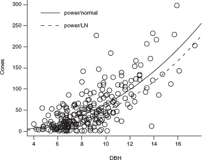
Figure 9.4 A nonlinear least-squares fit to the fir fecundity data (nls(TOTCONES~a* DBH~b,…)); the linear model fit to the log-log data (equivalent to a power-law fit with lognormal errors) is also shown.
Fitting models with both nonlinear covariates and categorical variables (the nonlinear analogue of ANCOVA—e.g., fitting different a and b parameters for wave and nonwave populations) is more difficult, but two functions from the nlme package, nlsList and gnls (generalized nonlinear least squares), can handle such models. nlsList does completely separate fits for separate groups—for example,
![]()
would fit separate a and b parameters for wave and nonwave populations—all parameters will vary among groups. The gnls command can fit models with only a subset of the parameters differing among groups—for example,
![]()
will fit different b parameters but the same a parameter for wave and nonwave populations.
The numerical methods that nls uses are similar to mle2's in that (1) you must specify starting values and (2) if the starting values are unrealistic, or if the problem is otherwise difficult, the numerical optimization may get stuck. Errors such as
step factor [] reduced below ‘minFactor' of
number of iterations exceeded maximum of…
or
Missing value or an infinity produced when evaluating the model
indicate numerical problems. To solve these problems try to find better starting conditions, reparameterize your model, or adjust the control options of nls (see ?nls.control).
As with ML models, you can often use simpler, more robust approaches like linear models to get a first estimate for the parameters (e.g., estimate the initial slope of a Michaelis-Menten function from the first 10% of the data and the asymptote from the last 10%, or estimate the parameters by linear regression based on a linearizing transformation). R includes some “self-starting” functions that do these steps automatically. The functions SSlogis and SSmicmen, for example, provide self-starting logistic and Michaelis-Menten functions. To fit a self-starting Michaelis-Menten model to the tadpole data with asymptote a and half-maximum b:
![]()
Use apropos(“SS”,ignore.case=FALSE) to see a more complete list of self-starting models. The names are cryptic, so check the help system for information about each model.
Further reading: Bates and Watts (1988), Pinheiro and Bates (2000).
9.4 Nonnormal Errors: Generalized Linear Models
Generalized linear models (not to be confused with general linear models) allow you to analyze models that have a particular kind of nonlinearity and particular kinds of nonnormally distributed (but still independent) errors.
Generalized linear models can fit any nonlinear relationship that has a linearizing transformation. That is, if y = f (x), there must be some function F such that F(f (x)) is a linear function of x. The procedure for fitting generalized linear models uses the function F to fit the data on the linearized scale (F(y) = F(f (x))) while calculating the expected variance on the untransformed scale in order to correct for the distortions that linearization would otherwise induce. In generalized-linear-model jargon F is called the link function. For example, when f is the logistic curve (y = f (x) = ex/(1 + ex)), the link function F is a the logit function (F(y) = log (y/(1–y)) = x; see p. 83 for the proof that the logit is really the inverse of the logistic). R knows about a variety of link functions including the log (x = log (y), which linearizes y = ex); square root (x = ![]() which linearizes y = x2); and inverse (x = 1/y, which linearizes y = 1/x): see ?family for more possibilities.
which linearizes y = x2); and inverse (x = 1/y, which linearizes y = 1/x): see ?family for more possibilities.
The class of nonnormal errors that generalized linear models can handle is called the exponential family. It includes Poisson, binomial, Gamma and normal distributions, but not negative binomial or beta-binomial distributions. Each distribution has a standard link function: the log link is standard for a Poisson, a logit link is standard for a binomial distribution, etc. The standard link functions make sense for typical applications. For example, the logit transformation converts unconstrained values into values between 0 and 1, which are appropriate as probabilities in a binomial model. However, R does allow you some flexibility to change these associations for specific problems.
GLMs are fit by a process called iteratively reweighted least squares, which overcomes the basic problem that transforming the data to make them linear also changes the variance. The key is that given an estimate of the regression parameters, and knowing the relationship between the variance and the mean for a particular distribution, one can calculate the variance associated with each point. With this variance estimate, one reestimates the regression parameters weighting each data point by the inverse of its variance; the new estimate gives new estimates of the variance; and so on. This procedure quickly and reliably fits the models, without the user needing to specify starting points.
Generalized linear models combine a range of nonnormal error distributions with the ability to work with some reasonable nonlinear functions. They also use the same simple model specification framework as lm, allowing us to explore combinations of factors, covariates, and interactions among variables. GLMs include logistic and binomial regression and log-linear models. They use terminology that should now be familiar to you; they estimate log-likelihoods and test the differences between models using the LRT.
The glm function implements generalized linear models in R. By far the two most common GLMs are Poisson regression, for count data, and logistic regression, for survival/failure data.
• Poisson regression: log link, Poisson error (Y — Poisson(aebx)):
![]()
The equivalent likelihood function is

• Logistic regression: logit link, binomial error (Y ~ Binom(p = exp (a + bx)/ (1 + exp (a + bx)), N)):
![]()
or

(You could also say p.pred=plogis(a+b*x) in the first line of logistregfun.)
GLMs can also fit models of exponentially decreasing survival, Y ~ Binom (p = exp (a + bx), N). Strong et al. (1999) modeled the survival probability of ghostmoth caterpillars as a decreasing function of density (and as a function of the presence or absence of entomopathogenic nematodes); Tiwari et al. (2006) modeled the probability that nesting sea turtles would not dig up an existing nest as a decreasing function of nest density. You can fit such a model this way:

Figure 9.5 Logistic (binomial) regression and log-binomial regression of fraction of tadpoles killed as a function of tadpole density. Logistic regression: glm(cbind(Killed,Initial-Killed)~Initial, family=“binomial”, data=ReedfrogFuncresp)
![]()
Use family=binomial(link=“log”) instead of family=“binomial” to specify the log instead of the logit link function. The equivalent negative log-likelihood function is

You can use either a logistic or a log-binomial model to fit Vonesh's tadpole mortality data (Figure 9.5), but the fact that expected survival decreases exponentially at high densities in both models causes problems of interpretation. If the probabilityof survival declines exponentially with density—which is true for the log-binomial model and approximately true at high densities for the logistic—then the expected number surviving is p(x) = x = e–(a+bx)x = cxe–bx. This is a Ricker function, which decreases to zero at high density rather than reaching an asymptote. In predator-prey systems for example, rather than this overcompensation response to density, we usually expect compensatory behavior—predation rate reaching an asymptote—the standard type II functional response model uses p(x) = A/(1 + Ahx), which has a weaker dependence on x, and which makes the limit of p(x)x as x becomes large equal to 1/h. The GLM, while convenient, may not be ecologically appropriate in this case.
After you fit a GLM, you can use the same generic set of modeling functions— summary, coef, confint, anova, and plot—to examine the parameters, test hypotheses, and plot residuals. anova(glm1,glm2,…) does an analysis of deviance (Likelihood Ratio tests) on a nested sequence of models. As with lm, the default parameters represent (1) the intercept (the baseline value of the first treatment), (2) differences in the intercept between the first and subsequent treatments, (3) the slope(s) with respect to the covariate(s) for the first group, or (4) differences in the slope between the first and subsequent treatments. However, all of the parameters are given on the scale of the link function (e.g., log scale for Poisson models, logit scale for binomial models). To interpret them, you need to transform them with the inverse link function (exponential for Poisson, logistic (=plogis) for binomial). For example, the coefficients of the logistic regression shown in Figure 9.5 are intercept = —0.095, slope = —0.0084. To find the probability of mortality at a tadpole density of 60, calculate exp (— 0.095 + —0.0084 ? 60)/(1 + exp (— 0.095 + —0.0084 ? 60) = 0.355.
Further reading: McCullagh and Nelder (1989); Dobson (1990); Hastie and Pregibon (1991); Lindsay (1997). R-specific: Crawley (2002); Faraway (2006).
9.4.1 Models for Overdispersion
To go beyond the exponential family of distributions (normal, binomial, Poisson, Gamma) you may well need to roll your own ML estimator. R has two built-in possibilities for the very common case of discrete data with overdispersion, i.e., more variance than would be expected from the standard (Poisson and binomial) models for discrete data.
9.4.1.1 QUASI LIKELIHOOD
Quasi-likelihood models “inflate” the expected variance of models to account for overdispersion (McCullagh and Nelder, 1989). For example, the expected variance of a binomial distribution with N samples and probability p is Np(1–p). The quasi-binomial model adds another parameter, ![]() , which inflates the variance to
, which inflates the variance to ![]() Np(1–p). The overdispersion parameter
Np(1–p). The overdispersion parameter ![]() (Burnham and Anderson (2004) call it C) is generally greater than 1–we usually find more variance than expected, rather than less. Quasi-Poisson models are defined similarly, with variance equal to
(Burnham and Anderson (2004) call it C) is generally greater than 1–we usually find more variance than expected, rather than less. Quasi-Poisson models are defined similarly, with variance equal to ![]() λ. This approach is called quasi likelihood because we don't specify a real likelihood model with a probability distribution for the data. We just specify the relationship between the mean and the variance. Nevertheless, the quasi-likelihood approach works well in practice. R uses the family function to specify quasi-likelihood models.
λ. This approach is called quasi likelihood because we don't specify a real likelihood model with a probability distribution for the data. We just specify the relationship between the mean and the variance. Nevertheless, the quasi-likelihood approach works well in practice. R uses the family function to specify quasi-likelihood models.
Because the quasi likelihood is not a true likelihood, we cannot use Likelihood Ratio tests or other likelihood-based methods for inference, but the parameter estimates and t statistics generated by summary should still work. However, various researchers have suggested that using an F test based on the ratio of deviances is appropriate: use anova(…,test=“F”) (Crawley, 2002; Venables and Ripley, 2002). Burnham and Anderson (2004) suggest using differences in “quasi-AIC” (qAIC) in this case, where the AqAIC uses the difference in deviance divided by the estimate of 0.
Since the log is the default link function for the quasipoisson family, you can fit a quasi-Poisson log-log model for fecundity as follows:
![]()
9.4.1.2 NEGATIVE BINOMIAL MODELS
Although the exponential family does not strictly include the negative binomial distribution, negative binomial models can be fit by a small extension of the GLM approach, iteratively fitting the k (overdispersion) parameter and then fitting the rest of the model with a fixed k parameter. The glm.nb function in the MASS package fits linear negative binomial models, although they restrict the model to a single k parameter for all groups. (Use $theta to extract the estimate of the negative binomial k parameter from a negative binomial model.)
Because we can use a log link (which is glm.nb's default link), we can exactly replicate our original log-likelihood model (cones ~ NegBin(a. DBHb, k)) with the following command:
![]()
The only difference from our earlier model is that the estimated intercept parameter is log (a) rather than a.
9.5 R Supplement
Here's how to fit various linear models to the log-transformed fir data. Since the data (TOTCONES) contain some zero values, taking logarithms would give us negative infinite values. We need either to drop these values (subset=T0TC0NES>0) or to add an off set of 1, in order to avoid infinities. However, since there are few zeros in the data (sum(firdata$T0TC0NES= =0) is 10 out of a total of 242 data points) and the mean number of cones is large, this adjustment shouldn't affect the results much. If zeros are frequent so that such an adjustment would affect your results significantly, or if the results vary depending on how large an off set you add, consider a different model (Section 9.4).

Since log(DBH) is a covariate and WAVE_NON is a factor, lm.d is a regression; lm.w is a one-way ANOVA; and lm.dw and lm.dwi are ANCOVA models with parallel and nonparallel slopes, respectively.
A few different ways to analyze the data:
![]()
Analysis of Variance Table

(I left lm.w out of the anova statement because it and lm.d cannot be nested.) anova compares the models sequentially, while AIC compares them simultaneously. AlCtab in the emdbook package offers several more options such as sorting the table in order of increasing AIC or computing AIC weights. Try coef, summary, and confint on these models as well.
The full ANCOVA model fit via mle2:


The maximum likelihood fit gives the same AIC as the lm fit. You can't always take this equality for granted, since different models that are formally equivalent may include different constants in the likelihood, and different functions may count the number of parameters differently. This is especially true when comparing results from different statistics packages.
As pointed out in the text, the models are parameterized differently:

You can check that the answers are equivalent; for example, the slope of the wave population is slope2 = 2.467 = log(DBH) + log(DBH):WAVE_N0Nw.
To do the full model comparison with mle2, you have to construct a series of nested models (analogous to lm.dw, lm.d, lm.w, lm.0). This is a bit tedious—one reason for using built-in functions where possible. You may want to read about the model.matrix function, which can simplify model construction. model.matrix uses a user-specified formula to construct a design matrix that, when multiplied by a vector of parameters, gives the expected value of each data point. By default the design matrix uses parameters that represent baseline levels and differences among groups, as in lm and glm. mle2's formula interface uses model.matrix internally, so that (e.g.) you can easily fit the full ANCOVA model by specifying
![]()
* This terminology is unfortunate since the rest of the world uses “GLM” to mean gene ralized linear models, which correspond to SAS's PROC GENMOD.
* anova gives so-called sequential sums of squares, which SAS calls “type I” sums of squares. If you need SAS-style “type III” sums of squares, you can use the Anova function in the car package. However, be aware that type III sums of squares are problematic, and indeed controversial (Venables, 1998).