
4 Probability and Stochastic Distributions
for Ecological Modeling
This chapter continues to review the math you need to fit models to data, moving forward from functions and curves to probability distributions. The first part discusses ecological variability in general terms, then reviews basic probability theory and some important applications, including Bayes' Rule and its application in statistics. The second part reviews how to analyze and understand probability distributions. The third part provides a bestiary of probability distributions, finishing with a short digression on some ways to extend these basic distributions.
4.1 Introduction: Why Does Variability Matter?
For many ecologists and statisticians, noise is just a nuisance—it gets in the way of drawing conclusions from the data. The traditional statistical approach to noise in data was to assume that all variation in the data was normally distributed, or transform the data until it was, and then use classical methods based on the normal distribution to draw conclusions. Some scientists turned to nonparametric statistics, which assume only that the shape of the data distribution is the same in all categories and provide tests of differences in the means or “location parameters” among categories. Unfortunately, such classical nonparametric approaches make it much harder to draw quantitative conclusions from data (rather than simply rejecting or failing to reject null hypotheses about differences between groups).
In the 1980s, as they acquired better computing tools, ecologists began to use more sophisticated models of variability such as generalized linear models (see Chapter 9). Chapter 3 illustrated a wide range of deterministic functions that correspond to deterministic models of the underlying ecological processes. This chapter will illustrate a wide range of models for the stochastic part of the dynamics. In these models, variability isn't just a nuisance but actually tells us something about ecological processes. For example, census counts that follow a negative binomial distribution (p. 124) tell us there is some form of environmental variation or aggregative response among individuals that we haven't taken into account (Shaw and Dobson, 1995).
Remember from Chapter 1 that what we treat as “signal” (deterministic) and what we treat as “noise” (stochastic) depends on the question. The same ecological variability, such as spatial variation in light, might be treated as random variation by a forester interested in the net biomass growth of a forest stand and as a deterministic driving factor by an ecophysiologist interested in the photosynthetic response of individual plants.
Noise affects ecological data in two different ways—as measurement error and as process noise (this distinction will become important in Chapter 11 when we deal with dynamical models). Measurement error is the variability or “noise” in our measurements, which makes it hard to estimate parameters and make inferences about ecological systems. Measurement error leads to large confidence intervals and low statistical power. Even if we can eliminate measurement error, process noise or process error (often so-called even though it isn't technically an error but a real part of the system) still exists. Variability affects any ecological system. For example, we can observe thousands of individuals to determine the average mortality rate with great accuracy. The fate of a group of a few individuals, however, depends both on the variability in mortality rates of individuals and on the demographic stochasticity that determines whether a particular individual lives or dies (“loses the coin toss”). Even though we know the average mortality rate perfectly, our predictions are still uncertain. Environmental stochasticity—spatial and temporal variability in (e.g.) mortality rate caused by variation in the environment rather than by the inherent randomness of individual fates—also affects the dynamics. Finally, even if we can minimize measurement error by careful measurement and minimize process noise by studying a large population in a constant environment (i.e., one with low levels of demographic and environmental stochasticity), ecological systems can still amplify variability in surprising ways (Bjornstad and Grenfell, 2001). For example, a tiny bit of demographic stochasticity at the beginning of an epidemic can trigger huge variation in epidemic dynamics (Rand and Wilson, 1991). Variability also feeds back to change the mean behavior of ecological systems. For example, in the damselfish system described in Chapter 2 the number of recruits in any given cohort is the number of settlers surviving density-dependent mortality, but the average number of recruits is lower than expected from an average-sized cohort of settlers because large cohorts suffer disproportionately high mortality and contribute relatively little to the average. This difference is an example of a widespread phenomenon called Jensen's inequality (Ruel and Ayres, 1999; Inouye, 2005).
4.2 Basic Probability Theory
To understand stochastic terms in ecological models, you'll have to (re)learn some basic probability theory. To define a probability, we first have to identify the sample space, the set of all the possible outcomes that could occur. Then the probability of an event A is the frequency with which that event occurs. A few probability rules are all you need to know:
1. If two events are mutually exclusive (e.g., “individual is male” and “individual is female”), then the probability that either occurs (the probability of A or B, or Prob(A ![]() B)) is the sum of their individual probabilities: Prob(male or female) = Prob(male) + Prob(female).
B)) is the sum of their individual probabilities: Prob(male or female) = Prob(male) + Prob(female).
We use this rule, for example, in finding the probability that an outcome is within a certain numeric range by adding up the probabilities of all the different (mutually exclusive) values in the range: for a discrete variable, for example, P(3 ≤ X ≤ 5) = P(X = 3) + P(X = 4) + P(X = 5).
2. If two events A and B are not mutually exclusive—the joint probability that they occur together, Prob(A ![]() B), is greater than zero—then we have to correct the rule for combining probabilities to account for double-counting:
B), is greater than zero—then we have to correct the rule for combining probabilities to account for double-counting:
![]()
For example, if we are tabulating the color and sex of animals, Prob(blue or male) = Prob(blue) + Prob(male)–Prob(blue male).
3. The probabilities of all possible outcomes of an observation or experiment add to 1.0: Prob(male) + Prob(female) = 1.0.
We will need this rule to understand the form of probability distributions, which often contain a normalization constant which ensures that the sum of the probabilities of all possible outcomes is 1.
4. The conditional probability of A given B, Prob(A|B), is the probability that A happens if we know or assume B happens. The conditional probability equals
![]()
For example, continuing the color and sex example:
![]()
By contrast, we may also refer to the probability of A when we make no assumptions about B as the unconditional probability of A: Prob(A) = Prob(A|B)Prob(B) + Prob(A|not B)Prob(not B). Conditional probability is central to understanding Bayes' Rule (Section 4.3).
5. If the conditional probability of A given B, Prob(A|B), equals the unconditional probability of A, then A is independent of B. Knowing about B provides no information about the probability of A. Independence implies that
![]()
which follows from substituting Prob(A|B) = Prob(A) in (4.2.1) and multiplying both sides by Prob(B). The probabilities of combinations of independent events are multiplicative.
Multiplying probabilities, or adding log-probabilities (log (Prob(A ![]() B)) = log (Prob(A)) + log (Prob(B)) if A and B are independent), is how we find the combined probability of a series of independent observations.
B)) = log (Prob(A)) + log (Prob(B)) if A and B are independent), is how we find the combined probability of a series of independent observations.
We can immediately use these rules to think about the distribution of seeds taken in the seed removal experiment (Chapter 2). The most obvious pattern in the data is that there are many zeros, probably corresponding to times when no predators visited the station. The sample space for seed disappearance is the number of seedstaken, from 0 to N (the number available). Suppose that when a predator did visit the station, which happened with probability v, it had an equal probability of taking any of the possible number of seeds (i.e., a uniform distribution from 0 to N). Since the probabilities must add to 1, this probability (Prob(x taken|predator visit)) is 1/(N + 1) (0 to N represents N +1 different possible events). What is the unconditional probability of x seeds being taken?
If x > 0, then only one type of event is possible—the predator visited and took x seeds—with overall probability v/(N + 1) (Figure 4.1a).
If x = 0, then there are two mutually exclusive possibilities. Either the predator didn't visit (probability 1–v), or it visited (probability v) and took zero seeds (probability 1/(N + 1)), so the overall probability is

Now make things a little more complicated and suppose that when a predator visits, it decides independently whether or not to take each seed. If the seeds of a given species are all identical, so that each seed is taken with the same probability p, then this process results in a binomial distribution. Using the rules above, the probability of x seeds being taken when each has probability p is px. It's also true that N–x seeds are not taken, with probability (1–p)N–x. Thus the probability is proportional to px. (1–p)N–x. To get the probabilities of all possible outcomes to add to 1, though, we have to multiply by a normalization constant N!/(x!(N–x)!),* or ![]() . (It ‘s too bad we can't just ignore these ugly normalization factors, which are always the least intuitive parts of probability formulas, but we really need them in order to get the right answers. Unless you are doing advanced calculations, however, you can usually take the formulas for the normalization constants for granted, without trying to puzzle out their meaning.)
. (It ‘s too bad we can't just ignore these ugly normalization factors, which are always the least intuitive parts of probability formulas, but we really need them in order to get the right answers. Unless you are doing advanced calculations, however, you can usually take the formulas for the normalization constants for granted, without trying to puzzle out their meaning.)
Now adding the “predator may or may not visit” layer to this formula, we have a probability

if x = 0 (since ![]() = 1, the normalization constant disappears from the second term), or
= 1, the normalization constant disappears from the second term), or
![]()
if x > 0 (Figure 4.1b).
This distribution is called the zero-inflated binomial (Inouye, 1999; Tyre et al., 2003). With only a few simple probability rules, we have derived a potentially useful distribution that might describe the pattern of seed predation better than any of the standard distributions we'll see later in this chapter.

Figure 4.1 Zero-inflated distributions. (a) zero-inflated uniform; (b) zero-inflated binomial. Number of seeds N = 5, probability of predator visit v = 0.7, binomial probability of individual seed predation p = 0.4.
4.3 Bayes' Rule
With the simple probability rules defined above we can also derive, and understand, Bayes' Rule. Most of the time we will use Bayes' Rule to go from the likelihood Prob(D|H), the probability of observing a particular set of data D given that a hypothesis H is true (p. 13), to the information we really want, Prob(H|D)—the probability of our hypothesis H in light of our data D. Bayes' Rule is just a recipe for turning around a conditional probability:
Bayes' Rule is general—H and D can be any events, not just hypothesis and data— but it's easier to understand Bayes' Rule when we have something concrete to tie it to. Deriving Bayes' Rule is almost as easy as remembering it. Rule 4 on p. 105 applied to P(H|D) implies
![]()
While applying it to P(D|H) tells us
![]()
But P(H ![]() D) = P(D
D) = P(D ![]() H), so
H), so
![]()
and dividing both sides by P(D) gives us (4.3.1).
Equation (4.3.1) says that the probability of the hypothesis given (in light of) the data is equal to the probability of the data given the hypothesis (the likelihood associated with H), times the probability of the hypothesis, divided by the probability of the data. There are two problems here: we don't know the probability of the hypothesis, P(H) (isn't that what we were trying to figure out in the first place?), and we don't know the unconditional probability of the data, P(D).
Let's think about the second problem first—our ignorance of P(D). We can calculate an unconditional probability for the data if we have a set of exhaustive, mutually exclusive hypotheses: in other words, we assume that one, and only one, of our hypotheses is true. Figure 4.2 shows a geometric interpretation of Bayes' Rule. The gray ellipse represents D, the set of all possibilities that could lead to the observed data.
If one of the hypotheses must be true, then the unconditional probability of observing the data is the sum of the probabilities of observing the data under any of the possible hypotheses. For N different hypotheses H1 to HN,

In words, the unconditional probability of the data is the sum of the likelihood of each hypothesis (P(D|Hj)) times its unconditional probability (P(Hj)). In Figure 4.2, taking each wedge (Hj), finding its area of overlap with the gray ellipse (D ![]() Hj), and summing the area of these “pizza slices” provides the area of the ellipse (D).
Hj), and summing the area of these “pizza slices” provides the area of the ellipse (D).
Substituting (4.3.5) into (4.3.1) gives the full form of Bayes' Rule for a particular hypothesis Hi when it is one of a mutually exclusive set of hypotheses {Hj}. The probability of the truth of Hi in light of the data is
![]()
In Figure 4 2, having observed the data D means we know that reality lies somewhere in the gray ellipse The probability that hypothesis 5 is true (i e , that we are somewhere in the hatched area) is equal to the area of the hatched/shaded “pizza slice” divided by the area of the ellipse. Bayes' Rule breaks this down further by supposing that we know how to calculate the likelihood of the data for each hypothesis—the ratio of the pizza slice divided by the area of the entire wedge (the area of the pizza slice [D ![]() H5] divided by the hatched wedge [H5]). Then we can recover the area of each slice by multiplying the likelihood by the prior (the area of the wedge) and calculate both P(D) and P(H5|D).
H5] divided by the hatched wedge [H5]). Then we can recover the area of each slice by multiplying the likelihood by the prior (the area of the wedge) and calculate both P(D) and P(H5|D).

Figure 4.2 Decomposition of the unconditional probability of the observed data (D) into the sum of the probabilities of the intersection of the data with each possible hypothesis ![]() . The entire gray ellipse in the middle represents D. Each wedge (e.g., the hatched area H5) represents an alternative hypothesis. The ellipse is divided into “pizza slices” (e.g., D
. The entire gray ellipse in the middle represents D. Each wedge (e.g., the hatched area H5) represents an alternative hypothesis. The ellipse is divided into “pizza slices” (e.g., D ![]() H5, hatched and shaded area). The area of each slice corresponds to D
H5, hatched and shaded area). The area of each slice corresponds to D ![]() Hj, the joint probability of the data D (ellipse) and the particular hypothesis Hj (wedge).
Hj, the joint probability of the data D (ellipse) and the particular hypothesis Hj (wedge).
Dealing with the second problem, our ignorance of the unconditional or prior probability of the hypothesis P(Hi), is more difficult. In the next section we will simply assume that we have other information about this probability, and we'll revisit the problem shortly in the context of Bayesian statistics. But first, just to practice with Bayes' Rule, we'll explore two simple examples that use Bayes' Rule to manipulate conditional probabilities.
4.3.1 False Positives in Medical Testing
Suppose the unconditional probability of a random person sampled from the population being infected (I) with some deadly but rare disease is one in a million: P(I) = 10–6. There is a test for this disease that never gives a false negative result: if you have the disease, you will definitely test positive (P(+ |I) = 1). However, the test does occasionally give a false positive result. One person in 100 who doesn't have the disease (is uninfected, U) will test positive anyway (P(+ |U) = 10–2). This sounds like a pretty good test. Let's compute the probability that someone who tests positive is actually infected.
Replace H in Bayes' Rule with “is infected” (I) and D with “tests positive” (+). Then
![]()
We know P(+|I) = 1 and P(I) = 10–6, but we don't know P(+), the unconditional probability of testing positive. You are either infected (I) or uninfected (U), so these events are mutually exclusive:
![]()
Then
![]()
because P(+ ![]() I) = P(+ |I)P(I) and similarly for U (4.2.1). We also know that P(U) = 1–P(I), so
I) = P(+ |I)P(I) and similarly for U (4.2.1). We also know that P(U) = 1–P(I), so

Since 10–6 is 10,000 times smaller than 10–2, and 10–8 is even tinier, we can neglect them.
Now that we've done the hard work of computing the denominator P(+), we can put it together with the numerator:

Even though false positives are unlikely, the chance that you are infected if you test positive is still only 1 in 10,000! For a sensitive test (one that produces few falsenegatives) for a rare disease, the probability that a positive test is detecting a true infection is approximately P(I)/P(false positive), which can be surprisingly small.
This false-positive issue also comes up in forensics cases. Assuming that a positive test is significant is called the base rate fallacy. It's important to think carefully about the sample population and the true probability of being guilty (or at least having been present at the crime scene) if your DNA matches DNA found at the crime scene.
4.3.2 Bayes' Rule and Liana Infestation
A student of mine used Bayes' Rule as part of a simulation model of liana (vine) dynamics in a tropical forest. He wanted to know the probability that a newly emerging sapling would be in a given “liana class” (L1 = liana-free, L2–L3 = light to moderate infestation, L4 = heavily infested with lianas). This probability depends on the number of trees nearby that are already infested (N). We have measurements of infestation of saplings from the field, and for each one we know the number of nearby infestations. Thus if we calculate the fraction of individuals in liana class Li with N nearby infested trees, we get an estimate of Prob(N|Li). We also know the overall fractions in each liana class, Prob(Li). When we add a new tree to the model, we know the neighborhood infestation N from the model. Thus we can figure out the rules for assigning infestation to a new sapling, Prob(Li|N), by using Bayes' Rule to calculate
![]()
For example, suppose we find that a new tree in the model has 3 infested neighbors. Let's say that the probabilities of each liana class (1 to 4) having 3 infested neighbors are Prob(3|Li) = {0.05,0.1,0.3,0.6} and that the overall fractions of each liana class in the forest (unconditional probabilities) are Li = {0.5,0.25,0.2,0.05}. Then the probability that the new tree is heavily infested (i.e., is in class L4) is
![]()
We would expect that a new tree with several infested neighbors has a much higher probability of heavy infestation than the overall (unconditional) probability of 0.05. Bayes' Rule allows us to quantify this guess.
4.3.3 Bayes' Rule in Bayesian Statistics
So what does Bayes' Rule have to do with Bayesian statistics?
Bayesians translate likelihood into information about parameter values using Bayes' Rule as given above. The problem is that we have the likelihood ![]() (data|hypothesis), the probability of observing the data given the model (parameters); what we want is Prob(hypothesis|data). After all, we already know what the data are!
(data|hypothesis), the probability of observing the data given the model (parameters); what we want is Prob(hypothesis|data). After all, we already know what the data are!
4.3.3.1 PRIORS
In the disease testing and the liana examples, we knew the overall, unconditional probability of disease or liana class in the population. When we're doing Bayesian statistics, however, we interpret P(Hi) instead as the prior probability of a hypothesis, our belief about the probability of a particular hypothesis before we see the data. Bayes' Rule is the formula for updating the prior in order to compute the posterior probability of each hypothesis, our belief about the probability of the hypothesis after we see the data. Suppose I have two hypotheses A and B and have observed some data D with likelihoods ![]() A = 0.1 and
A = 0.1 and ![]() B = 0.2. In other words, the probability of D occurring if hypothesis A is true (P(D|A)) is 10%, while the probability of D occurring if hypothesis B is true (P(D|B)) is 20%. If I assign the two hypotheses equal prior probabilities (0.5 each), then Bayes' Rule says the posterior probability of A is
B = 0.2. In other words, the probability of D occurring if hypothesis A is true (P(D|A)) is 10%, while the probability of D occurring if hypothesis B is true (P(D|B)) is 20%. If I assign the two hypotheses equal prior probabilities (0.5 each), then Bayes' Rule says the posterior probability of A is
![]()
and the posterior probability of B is 2/3. However, if I had prior information that said A was twice as probable (Prob(A) = 2/3, Prob(B) = 1/3), then the probability of A given the data would be 0.5 (do the calculation). If you rig the prior, you can get whatever answer you want: e.g., if you assign B a prior probability of 0, then no data will ever convince you that B is true (in which case you probably shouldn't have done the experiment in the first place). Frequentists claim that this possibility makes Bayesian statistics open to cheating (Dennis, 1996); however, every Bayesian analysis must clearly state the prior probabilities it uses. If you have good reason to believe that the prior probabilities are not equal, from previous studies of the same or similar systems, then arguably you should use that information rather than starting as frequentists do from the ground up every time. (The frequentist-Bayesian debate is one of the oldest and most virulent controversies in statistics (Dennis, 1996; Ellison 1996); I can't possibly do it justice here.)
However, trying so-called flat or weak or uninformative priors—priors that assume you have little information about which hypothesis is true—as a part of your analysis is a good idea, even if you do have prior information (Edwards, 1996). You may have noticed in the first example above that when we set the prior probabilities equal, the posterior probabilities were just equal to the likelihoods divided by the sum of the likelihoods. If all the P(Hi) are equal to the same constant C, then
![]()
where Li is the likelihood of hypothesis i.
You may think that setting all the priors equal would be an easy way to eliminate the subjective nature of Bayesian statistics and make everybody happy. Two examples, however, will demonstrate that it's not that easy to say what it means to be completely “objective” or ignorant of which hypothesis is true.
• Partitioning hypotheses: Suppose we find a nest missing eggs that might have been taken by a raccoon, a squirrel, or a snake (only). The three hypotheses “raccoon” (R), “squirrel” (Q), and “snake” (S) are our mutually exclusive and exhaustive set of hypotheses for the identity of the predator. If we have no other information (e.g., about the local densities or activity levels of different predators), we might choose equal prior probabilities for all three hypotheses. Since there are three mutually exclusive predators, Prob(R) = Prob(Q) = Prob(S) = 1/3. Now a friend comes and asks us whether we really believe that mammalian predators are twice as likely to eat the eggs as reptiles (Prob(R) + Prob(Q) = 2Prob(S)) (Figure 4.3). What do we do? We might solve this particular problem by setting the probability for snakes (the only reptiles) to 0.5, the probability for mammals (Prob(R ![]() Q)) to 0.5, and the probability for raccoons and squirrels equal (Prob(R) = Prob(Q) = 0.25), but this simple example suggests that such pitfalls are ubiquitous.
Q)) to 0.5, and the probability for raccoons and squirrels equal (Prob(R) = Prob(Q) = 0.25), but this simple example suggests that such pitfalls are ubiquitous.

Figure 4.3 The difficulty of defining an uninformative prior for discrete hypotheses. Dark bars are priors that assume predation by each species is equally likely; light bars divide predation by group first, then by species within group.
• Changing scales: A similar problem arises with continuous variables. Suppose we believe that the mass of a particular bird species is between 10 and 100 g, and that no particular value is any more likely than other: the prior distribution is uniform, or flat. That is, the probability that the mass is in some range of width Δm is constant: Prob(mass = m) = 1/90Δm (so that ![]() = 1: see p. 116 for more on probability densities).
= 1: see p. 116 for more on probability densities).
But is it sensible to assume that the probability that a species' mass is between 10 and 20 is the same as the probability that it is between 20 and 30, or should it be the same as the probability that it is between 20 and 40—that is, would it make more sense to think of the mass distribution on a logarithmic scale? If we say that the probability distribution is uniform on a logarithmic scale, then a species is less likely to be between 20 and 30 than it is to be between 10 and 20 (Figure 4.4).* Since changing the scale is not really changing anything about the world, just the way we describe it, this change in the prior is another indication that it's harder than we think to say what it means to be ignorant. In any case, many Bayesians think that researchers try too hard to pretend ignorance, and that one really should use what is known about the system. Crome et al. (1996) compare extremely different priors in a conservation context to show that their data really are (or should be) informative to a wide spectrum of stakeholders, regardless of their perspectives.

Figure 4.4 The difficulty of defining an uninformative prior on continuous scales. If we assume that the probabilities are uniform on one scale (linear or logarithmic), they must be nonuniform on the other.
4.3.3.2 INTEGRATING THE DENOMINATOR
The other challenge with Bayesian statistics, which is purely technical and does not raise any deep conceptual issues, is the problem of adding up the denominator ![]() in Bayes' Rule. If the set of hypotheses (parameters) is continuous, then the denominator is
in Bayes' Rule. If the set of hypotheses (parameters) is continuous, then the denominator is ![]() where h is a particular parameter value.
where h is a particular parameter value.
For example, the binomial distribution says that the likelihood of obtaining 2 heads in 3 (independent, equal-probability) coin flips is ![]() a function of p. The likelihood for p = 0.5 is therefore 0.375, but to get the posterior probability we have to divide by the probability of getting 2 heads in 3 flips for any value of p. Assuming a flat prior, the denominator is
a function of p. The likelihood for p = 0.5 is therefore 0.375, but to get the posterior probability we have to divide by the probability of getting 2 heads in 3 flips for any value of p. Assuming a flat prior, the denominator is ![]() , so the posterior probability density of p = 0.5 is 0.375/0.25 = 1.5.32*
, so the posterior probability density of p = 0.5 is 0.375/0.25 = 1.5.32*
For the binomial case and other simple probability distributions, it's easy to sum or integrate the denominator either analytically or numerically. If we care only about the relative probability of different hypotheses, we don't need to integrate the denominator because it has the same constant value for every hypothesis.
Often, however, we do want to know the absolute probability. Calculating the unconditional probability of the data (the denominator for Bayes' Rule) can be extremely difficult for more complicated problems. Much of current research in Bayesian statistics focuses on ways to calculate the denominator. We will revisit this problem in Chapters 6 and 7, first integrating the denominator by brute-force numerical integration, then looking briefly at a sophisticated technique for Bayesian analysis called Markov chain Monte Carlo.
4.3.4 Conjugate Priors
Using so-called conjugate priors makes it easy to do the math for Bayesian analysis. Imagine that we're flipping coins (or measuring tadpole survival or counting numbers of different morphs in a fixed sample) and that we use the binomial distribution to model the data. For a binomial with a per-trial probability of p and N trials, the probability of x successes is proportional (leaving out the normalization constant) to px(1–p)N–x. Suppose that instead of describing the probability of x successes with a fixed per-trial probability p and number of trials N we wanted to describe the probability of a given per-trial probability p with fixed x and N. We would get Prob(p) proportional to px(1–p)N–x—exactly the same formula, but with a different proportionality constant and a different interpretation. Instead of a discrete probability distribution over a sample space of all possible numbers of successes (0 to N), now we have a continuous probability distribution over all possible probabilities (all values between 0 and 1). The second distribution, for Prob(p), is called the Beta distribution (p. 133) and it is the conjugate prior for the binomial distribution.
Mathematically, conjugate priors have the same structure as the probability distribution of the data. They lead to a posterior distribution with the same mathematical form as the prior, although with different parameter values. Intuitively, you get a conjugate prior by turning the likelihood around to ask about the probability of a parameter instead of the probability of the data.
We'll come back to conjugate priors and how to use them in Chapters 6 and 7.
4.4 Analyzing Probability Distributions
You need the same kinds of skills and intuitions about the characteristics of probability distributions that we developed in Chapter 3 for mathematical functions.
4.4.1 Definitions
DISCRETE
A probability distribution is the set of probabilities on a sample space or set of outcomes. Since this book is about modeling quantitative data, we will always be dealing with sample spaces that are numbers—the number or amount observed in some measurement of an ecological system. The simplest distributions to understand are discrete distributions whose outcomes are a set of integers; most of the discrete distributions we deal with describe counting or sampling processes and have ranges that include some or all of the nonnegative integers.
A discrete distribution is most easily described by its distribution function, which is just a formula for the probability that the outcome of an experiment or observation (called a random variable) X is equal to a particular value x (f (x) = Prob(X = x)). A distribution can also be described by its cumulative distribution function F(x) (note the uppercase F), which is the probability that the random variable X is less than or equal to a particular value x (F(x) = Prob(X ≤ x)). Cumulative distribution functions are most useful for frequentist calculations of tail probabilities, e.g., the probability of getting n or fewer heads in a coin-tossing experiment with a given trial probability.
CONTINUOUS
A probability distribution over a continuous range (such as all real numbers, or the nonnegative real numbers) is called a continuous distribution. The cumulative distribution function of a continuous distribution (F(x) = Prob(X ≤ x)) is easy to define and understand—it's just the probability that the observed value of a continuous random variable X is smaller than a particular value x in any given observation or experiment. The probability density function (the analogue of the distribution function for a discrete distribution), although useful, is more confusing, since the probability of any precise value is zero. You may imagine that a measurement of (say) pH is exactly 7.9, but in fact what you have observed is that the pH is between 7.82 and 7.98—if your meter has a precision of ±1%. Thus continuous probability distributions are expressed as probability densities rather than probabilities—the probability that random variable X is between x and x + Δx, divided by Δx (Prob(7.82 < X < 7.98)/0.16, in this case). Dividing by Δx allows the observed probability density to have a well-defined limit as precision increases and Δx shrinks to zero. Unlike probabilities, probability densities can be larger than 1 (Figure 4.5). For example, if the pH probability distribution is uniform on the interval [7,7.1] but zero everywhere else, its probability density is 10 in this range. In practice, we will be concerned mostly with relative probabilities or likelihoods, and so the maximum density values and whether they are greater than or less than 1 won't matter much.
4.4.2 Means (Expectations)
The first thing you usually want to know about a distribution is its average value, also called its mean or expectation.

Figure 4.5 Probability, probability density, and cumulative distributions. Discrete (binomial: N = 5, p = 0.3) (a) probability and (b) cumulative probability distributions. Continuous (exponential: λ = 1.5) (c) probability density and (d) cumulative probability distributions.
In general the expectation operation, denoted by E[.] (or a bar over a variable, such as ![]() ) gives the “expected value” of a set of data, or a probability distribution, which in the simplest case is the same as its (arithmetic) mean value. For a set of N data values written down separately as {x1,x2,x3,…,xN}, the formula for the mean is familiar:
) gives the “expected value” of a set of data, or a probability distribution, which in the simplest case is the same as its (arithmetic) mean value. For a set of N data values written down separately as {x1,x2,x3,…,xN}, the formula for the mean is familiar:
![]()
Suppose we have the data tabulated instead, so that for each possible value of x (for a discrete distribution) we have a count of the number of observations (possibly zero, possibly more than 1), which we call c(x). Summing over all of the possible values of x, we have
![]()
where Prob(x) is the discrete probability distribution representing this particular data set. More generally, you can think of Prob(x) as representing some particular theoretical probability distribution which only approximately matches any actual data set.
We can compute the mean of a continuous distribution as well. First, let's think about grouping (or “binning”) the values in a discrete distribution into categories of size Δx. Then if p(x), the density of counts in bin x, is c(x)/(NΔx), the formula for the mean becomes ∑ p(x). xΔx. If we have a continuous distribution with Δx very small, this becomes ∫ p(x)xdx. (This is in fact the definition of an integral.) For example, an exponential distribution p(x) = λ exp (– λx) has an expectation or mean value of ∫ λ exp (– λx)xdx = 1/λ. (You don't need to know how to do this integral analytically: the R supplement will briefly discuss numerical integration in R.)
4.4.3 Variances (Expectation of X2)
The mean is the expectation of the random variable X itself, but we can also ask about the expectation of functions of X. The first example is the expectation of X2. We just fill in the value x2 for x in all of the formulas above: E[x2] = ∑ Prob(x)x2 for a discrete distribution, or ∫ p(x)x2 dx for a continuous distribution. (We are not asking for ∑ Prob(x2)x2.) The expectation of x2 is a component of the variance, which is the expected value of (x–E[x])2 or (x–![]() )2, or the expected squared deviation around the mean. (We can also show that
)2, or the expected squared deviation around the mean. (We can also show that
![]()
by using the rules for expectations that (1) E[x + y] = E[x]+E[y] and (2) if c is a constant, E[cx] = cE[x]. The right-hand formula is simpler to compute than E[(x–![]() )2], but more subject to roundoff error.)
)2], but more subject to roundoff error.)
Variances are easy to work with because they are additive (Var(a + b) = Var(a) + Var(b) if a and b are uncorrelated), but harder to compare with means since their units are the units of the mean squared. Thus we often use instead the standard deviation of a distribution, ![]() which has the same units as X.
which has the same units as X.
Two other summaries related to the variance are the variance-to-mean ratio and the coefficient of variation (CV), which is the ratio of the standard deviation to the mean. The variance-to-mean ratio has units equal to the mean; it is used primarily to characterize discrete sampling distributions and compare them to the Poisson distribution, which has a variance-to-mean ratio of 1. The CV is more common and is useful when you want to describe variation that is proportional to the mean. For example, if you have a pH meter that is accurate to ±10%, so that a true pH value of x will give measured values that are normally distributed with 2σ = 0.1x* then σ = 0.05 ![]() and the CV is 0.05.
and the CV is 0.05.
4.4.4 Higher Moments
The expectation of (x–E[x])3 tells you the skewness of a distribution or a data set, which indicates whether it is asymmetric around its mean. The expectation E[(x–E[x])4] measures the kurtosis, the “pointiness” or “flatness,” of a distribution.![]() These are called the third and fourth central moments of the distribution. Ingeneral, the nth moment is E[xn], and the nth central moment is E[(x–
These are called the third and fourth central moments of the distribution. Ingeneral, the nth moment is E[xn], and the nth central moment is E[(x–![]() )n]; the mean is the first moment, and the variance is the second central moment. We won't be too concerned with these summaries (of data or distributions), but they do come up sometimes.
)n]; the mean is the first moment, and the variance is the second central moment. We won't be too concerned with these summaries (of data or distributions), but they do come up sometimes.
4.4.5 Median and Mode
The median and mode are two final properties of probability distributions that are not related to moments. The median of a distribution is the point that divides the area of the probability density in half, or the point at which the cumulative distribution function is equal to 0.5. It is often useful for describing data, since it is robust—outliers change its value less than they change the mean—but for many distributions it's more complicated to compute than the mean. The mode is the “most likely value,” the maximum of the probability distribution or density function. For symmetric distributions the mean, mode, and median are all equal; for right-skewed distributions, in general mode < median < mean.
4.4.6 The Method of Moments
Suppose you know the theoretical values of the moments (e.g., mean and variance) of a distribution and have calculated the sample values of the moments (by calculating ![]() = ∑ x/N and s2 = ∑ (x –
= ∑ x/N and s2 = ∑ (x –![]() )2/N; don't worry for the moment about whether the denominator in the sample variance should be N or N–1). Then there is a simple way to estimate the parameters of a distribution, called the method of moments: just match the sample values up with the theoretical values. For the normal distribution, where the parameters of the distribution are just the mean and the variance, this is trivially simple: μ =
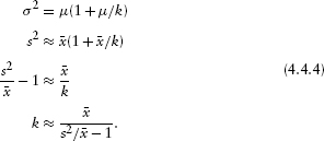
)2/N; don't worry for the moment about whether the denominator in the sample variance should be N or N–1). Then there is a simple way to estimate the parameters of a distribution, called the method of moments: just match the sample values up with the theoretical values. For the normal distribution, where the parameters of the distribution are just the mean and the variance, this is trivially simple: μ = ![]() , σ2 = s2. For a distribution like the negative binomial, however (p. 124), it involves a little bit of algebra. The negative binomial has parameters μ (equal to the mean, so that's easy) and k; the theoretical variance is σ2 = μ (1 + μ/k). Therefore, setting μ
, σ2 = s2. For a distribution like the negative binomial, however (p. 124), it involves a little bit of algebra. The negative binomial has parameters μ (equal to the mean, so that's easy) and k; the theoretical variance is σ2 = μ (1 + μ/k). Therefore, setting μ ![]()
![]() , s2
, s2 ![]() μ (1 + μ/k), and solving for k, we calculate the method-of-moments estimate of k:
μ (1 + μ/k), and solving for k, we calculate the method-of-moments estimate of k:
The method of moments is very simple but is often biased; it's a good way to get a first estimate of the parameters of a distribution, but for serious work you should follow it up with a maximum likelihood estimator (Chapter 6).
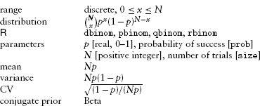
TABLE 4.1
Summary of Probability Distributions

4.5 Bestiary of Distributions
The rest of the chapter presents brief introductions to a variety of useful probability distribution (Table 4.1), including the mechanisms behind them and some of their basic properties. Like the bestiary in Chapter 3, you can skim this bestiary on the first reading. The appendix of Gelman et al. (1996) contains a useful table, more abbreviated than these descriptions but covering a wider range of functions. The book by Evans et al. (2000) is also useful.
4.5.1 Discrete Models
4.5.1.1 BINOMIAL
The binomial (Figure 4.6) is probably the easiest distribution to understand. It applies when you have samples with a fixed number of subsamples or “trials” in each one, and each trial can have one of two values (black/white, heads/tails, alive/dead, species A/species B), and the probability of “success” (black, heads, alive, species A) is the same in every trial. If you flip a coin 10 times (N = 10) and the probability of a head in each coin flip is p = 0.7, then the probability of getting 7 heads (k = 7) will have a binomial distribution with parameters N = 10 and p = 0.7.* Don't confuse the trials (subsamples), and the probability of success in each trial, with the number of samples and the probabilities of the number of successful trials in each sample. In the seed predation example, a trial is an individual seed and the trial probability is the probability that an individual seed is taken, while a sample is the observation of a particular station at a particular time and the binomial probabilities are the probabilities that a certain total number of seeds disappears from the station. You can derive the part of the distribution that depends on x, px(1–p)N–x, by multiplying the probabilities of x independent successes with probability p and N–x independent failures with probability 1–p. The rest of the distribution function, ![]() = N!/(x!(N–x)!), is a normalization constant that we can justify either with a combinatorial argument about the number of different ways of sampling x objects out of a set of N, or simply by saying that we need a factor in front of the formula to make sure the probabilities add up to 1.
= N!/(x!(N–x)!), is a normalization constant that we can justify either with a combinatorial argument about the number of different ways of sampling x objects out of a set of N, or simply by saying that we need a factor in front of the formula to make sure the probabilities add up to 1.

Figure 4.6 Binomial distribution. Number of trials (N) equals 10 for all distributions.
The mean of the binomial is Np and its variance is Np(1–p). Like most discrete sampling distributions (e.g., the binomial, Poisson, negative binomial), this variance is proportional to the number of trials per sample N. When the number of trials per sample increases the variance also increases, but the coefficient of variation ![]() decreases. The dependence on p(l–p) means the binomial variance is small when p is close to 0 or 1 (and therefore the values are scrunched up near 0 or N) and largest when p = 0.5. The coefficient of variation, on the other hand, is largest for small p.
decreases. The dependence on p(l–p) means the binomial variance is small when p is close to 0 or 1 (and therefore the values are scrunched up near 0 or N) and largest when p = 0.5. The coefficient of variation, on the other hand, is largest for small p.
When N is large and p isn't too close to 0 or 1 (i.e., when Np is large), then the binomial distribution is approximately normal (Figure 4.17).
A binomial distribution with only one trial (N = 1) is called a Bernoulli trial.
You should use the binomial in fitting data only when the number of possible successes has an upper limit. When N is large and p is small, so that the probability of getting N successes is small, the binomial approaches the Poisson distribution, which is covered in the next section (Figure 4.17).
Examples: number of surviving individuals/nests out of an initial sample; number of infested/infected animals, fruits, etc. in a sample; number of a particular class (haplotype, subspecies, etc.) in a larger population.
Summary:
4.5.1.2 POISSON
The Poisson distribution (Figure 4.7) gives the distribution of the number of individuals, arrivals, events, counts, etc., in a given time/space/unit of counting effort if each event is independent of all the others. The most common definition of the Poisson has only one parameter, the average density or arrival rate, λ, which equals the expected number of counts in a sampling unit. An alternative parameterization gives a density per unit sampling effort and then specifies the mean as the product of the density per sampling effort r times the sampling effort t, λ = rt. This parameterization emphasizes that even when the population density is constant, you can change the Poisson distribution of counts by sampling more extensively—for longer times or over larger quadrats.
The Poisson distribution has no upper limit, although values much larger than the mean value are highly improbable. This characteristic provides a rule for choosing between the binomial and Poisson. If you expect to observe a “ceiling” on the number of counts, you should use the binomial; if you expect the number of counts to be effectively unlimited, even if it is theoretically bounded (e.g., there can't really be an infinite number of plants in your sampling quadrat), use the Poisson.
The variance of the Poisson is equal to its mean. However, the coefficient of variation decreases as the mean increases, so in that sense the Poisson distribution becomes more regular as the expected number of counts increases. The Poisson distribution makes sense only for count data. Since the CV is unitless, it should not depend on the units we use to express the data; since the CV of the Poisson is ![]() if we used a Poisson distribution to describe data on measured lengths, we could reduce the CV by a factor of 10 by changing units from meters to centimeters (which would be silly).
if we used a Poisson distribution to describe data on measured lengths, we could reduce the CV by a factor of 10 by changing units from meters to centimeters (which would be silly).

Figure 4.7 Poisson distribution.
For λ < 1 the Poisson's mode is at zero. When the expected number of counts gets large (e.g., λ > 10) the Poisson becomes approximately normal (Figure 4.17).
Examples: number of seeds/seedlings falling in a gap; number of off spring produced in a season (although this might be better fit by a binomial if the number of breeding attempts is fixed); number of prey caught per unit time.
Summary:


4.5.1.3 NEGATIVE BINOMIAL
Most probability books derive the negative binomial distribution (Figure 4.8) from a series of independent binary (heads/tails, black/white, male/female, yes/no) trials that all have the same probability of success, like the binomial distribution. However, rather than counting the number of successes obtained in a fixed number of trials as in a binomial distribution, the negative binomial counts the number of failures before a predetermined number of successes occurs.
This failure-process parameterization is only occasionally useful in ecological modeling. Ecologists use the negative binomial because it is discrete, like the Poisson, but its variance can be larger than its mean (i.e., it can be overdispersed). Thus, it's a good phenomenological description of a patchy or clustered distribution with no intrinsic upper limit that has more variance than the Poisson.
The “ecological” parameterization of the negative binomial replaces the parameters p (probability of success per trial: prob in ![]() ) and n (number of successes before you stop counting failures: size in
) and n (number of successes before you stop counting failures: size in ![]() ) with μ = n(1–p)/p, the mean number of failures expected (or of counts in a sample: mu in
) with μ = n(1–p)/p, the mean number of failures expected (or of counts in a sample: mu in ![]() ), and k, which is typically called an overdispersion parameter. Confusingly, k is also called size in
), and k, which is typically called an overdispersion parameter. Confusingly, k is also called size in ![]() , because it is mathematically equivalent to n in the failure-process parameterization.
, because it is mathematically equivalent to n in the failure-process parameterization.
The overdispersion parameter measures the amount of clustering, or aggregation, or heterogeneity, in the data: a smaller k means more heterogeneity. The variance of the negative binomial distribution is μ + μ2/k, so as k becomes large the variance approaches the mean and the distribution approaches the Poisson distribution. For k > 10 μ, the negative binomial is hard to tell from a Poisson distribution, but k is often less than μ in ecological applications.*
Specifically, you can get a negative binomial distribution as the result of a Poisson sampling process where the rate λ itself varies. If λ is Gamma-distributed (p. 131) with shape parameter k and mean μ, and x is Poisson-distributed with mean λ, then the distribution of x will be a negative binomial distribution with mean μ and overdispersion parameter k (May, 1978; Hilborn and Mangel, 1997). In this case, the negative binomial reflects unmeasured (“random”) variability in the population.
Negative binomial distributions can also result from a homogeneous birth-death process, births and deaths (and immigrations) occurring at random in continuous time. Samples from a population that starts from 0 at time t = 0, with immigration rate i, birthrate b, and death rate d will be negative binomially distributed with parameters μ = i/(b–d)(e(b–d)t – 1) and k = i/b (Bailey, 1964, p. 99).
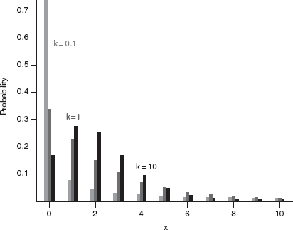
Figure 4.8 Negative binomial distribution. Mean | = 2 in all cases.
Several different ecological processes can often generate the same probability distribution. We can usually reason forward from knowledge of probable mechanisms operating in the field to plausible distributions for modeling data, but this many-to-one relationship suggests that it is unsafe to reason backwards from probability distributions to particular mechanisms that generate them.
Examples: essentially the same as the Poisson distribution, but allowing for heterogeneity. Numbers of individuals per patch; distributions of numbers of parasites within individual hosts; number of seedlings in a gap, or per unit area, or per seed trap.
Summary:


![]() 's default is the coin-flipping (n=size, p=prob) parameterization. In order to use the “ecological” (μ=mu, k=size) parameterization, you must name the mu parameter explicitly (e.g., dnbinom(5,size=0.6,mu=1)).
's default is the coin-flipping (n=size, p=prob) parameterization. In order to use the “ecological” (μ=mu, k=size) parameterization, you must name the mu parameter explicitly (e.g., dnbinom(5,size=0.6,mu=1)).
4.5.1.4 GEOMETRIC
The geometric distribution (Figure 4.9) is the number of trials (with a constant probability of failure) until you get a single failure: it's a special case of the negative binomial, with k or n = 1.
Examples: number of successful/survived breeding seasons for a seasonally reproducing organism. Lifespans measured in discrete units.
Summary:

4.5.1.5 BETA-BINOMIAL
Just as one can compound the Poisson distribution with a Gamma distribution to allow for heterogeneity in rates, producing a negative binomial, one can compound the binomial distribution with a Beta distribution (p. 133) to allow for heterogeneity in per-trial probability, producing a beta-binomial distribution (Figure 4.10) (Crowder, 1978; Reeve and Murdoch, 1985; Hatfield et al., 1996). The most common parameterization of the beta-binomial distribution uses the binomial parameter N (trials per sample), plus two additional parameters a and b that describe the Beta distribution of the per-trial probability. When a = b = 1 the per-trial probability is equally likely to be any value between 0 and 1 (the mean is 0.5), and the beta-binomial gives a uniform (discrete) distribution between 0 and N. As a + b increases, the variance of the underlying heterogeneity decreases and the beta-binomial converges to the binomial distribution. Morris (1997) suggests a different parameterization that uses an overdispersion parameter θ, like the k parameter of the negative binomial distribution. In this case the parameters are N, the per-trial probability p (= a/(a + b)), and θ (= a + b). When θ is large (small overdispersion), the beta-binomial becomes binomial. When θ is near zero (large overdispersion), the beta-binomial becomes U-shaped (Figure 4.10).

Figure 4.9 Geometric distribution.
Examples: as for the binomial.
Summary:


Figure 4.10 Beta-binomial distribution. Number of trials (N) equals 10, average per-trial probability (p) equals 0.5 for all distributions.
4.5.2 Continuous Distributions
4.5.2.1 UNIFORM DISTRIBUTION
The uniform distribution (Figure 4.11) with limits a and b, denoted U(a, b), has a constant probability density of 1/(b–a) for a ≤ x ≤ b and zero probability elsewhere. The standard uniform, U(0,1), is frequently used as a building block for other distributions but the uniform distribution is surprisingly rarely used in ecology otherwise.
Summary:
![]()

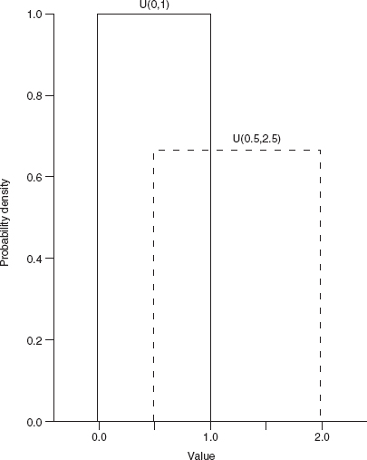
Figure 4.11 Uniform distribution.
4.5.2.2 NORMAL DISTRIBUTION
Normally distributed variables (Figure 4.12) are everywhere, and most classical statistical methods use this distribution. The explanation for the normal distribution's ubiquity is the Central Limit Theorem, which says that if you add a large number of independent samples from the same distribution, the distribution of the sum will be approximately normal. “Large,” for practical purposes, can mean as few as 5. The Central Limit Theorem does not mean that “all samples with large numbers are normal.” One obvious counterexample is two different populations with different means that are lumped together, leading to a distribution with two peaks (p. 138). Also, adding isn't the only way to combine samples: if you multiply many independent samples from the same distribution, you get a lognormal distribution instead (p. 135).

Figure 4.12 Normal distribution.
Many distributions (binomial, Poisson, negative binomial, Gamma) become approximately normal in some limit (Figure 4.17). You can usually think about this as some form of “adding lots of things together.”
The normal distribution specifies the mean and variance separately, with two parameters, which means that one often assumes constant variance (as the mean changes), in contrast to the Poisson and binomial distribution where the variance is a fixed function of the mean.
Examples: many continuous, symmetrically distributed measurements—temperature, pH, nitrogen concentration.
Summary:

4.5.2.3 GAMMA
The Gamma distribution (Figure 4.13) is the distribution of waiting times until a certain number of events take place. For example, Gamma(shape = 3, scale = 2) is the distribution of the length of time (in days) you'd expect to have to wait for 3 deaths in a population, given that the average survival time is 2 days (or mortality rate is 1/2 per day). The mean waiting time is 6 days = (3 deaths/(1/2 death per day)). (While the gamma function (gamma in R; see the appendix) is usually written with a capital Greek gamma, r, the Gamma distribution (dgamma in R) is written out as Gamma.) Gamma distributions with integer shape parameters are also called Erlang distributions. The Gamma distribution is still defined, and useful, for noninteger (positive) shape parameters, but the simple description given above breaks down: how can you define the waiting time until 3.2 events take place?
For shape parameters ≤ 1, the Gamma has its mode at zero; for shape parameter = 1, the Gamma is equivalent to the exponential (see p. 133). For shape parameters greater than 1, the Gamma has a peak (mode) at a value greater than zero; as the shape parameter increases, the Gamma distribution becomes more symmetrical and approaches the normal distribution. This behavior makes sense if you think of the Gamma as the distribution of the sum of independent, identically distributed waiting times, in which case it is governed by the Central Limit Theorem.
The scale parameter (sometimes defined in terms of a rate parameter instead, 1 /scale) adjusts the mean of the Gamma by adjusting the waiting time per event; however, multiplying the waiting time by a constant to adjust its mean also changes the variance, so both the variance and the mean depend on the scale parameter.
The Gamma distribution is less familiar than the normal, and new users of the Gamma often find it annoying that in the standard parameterization you can't adjust the mean independently of the variance. You could define a new set of parameters m (mean) and v (variance), with scale = v/m and shape = m2/v—but then you would find (unlike the normal distribution) the shape changing as you changed the variance. Nevertheless, the Gamma is extremely useful; it solves the problem that many researchers face when they have a continuous, positive variable with “too much variance,” whose coefficient of variation is greater than about 0.5. Modeling such data with a normal distribution leads to unrealistic negative values, which then have to be dealt with in some ad hoc way like truncating them or otherwise trying to ignore them. The Gamma is often a more convenient and realistic alternative.

Figure 4.13 Gamma distribution.
The Gamma is the continuous counterpart of the negative binomial, which is the discrete distribution of a number of trials (rather than length of time) until a certain number of events occur. Both the negative binomial and Gamma distributions are often generalized, however, in ways that are useful phenomenologically but that don't necessarily make sense according to their simple mechanistic descriptions.
The Gamma and negative binomial are both frequently used as phenomenologicaly, skewed, or over dispersed versions of the normal or Poisson distributions. The Gamma is less widely used than the negative binomial because the negative binomial replaces the Poisson, which is restricted to a particular variance, while the Gamma replaces the normal, which can have any variance. Thus you might use the negative binomial for any discrete distribution with a variance greater than its mean, whereas you wouldn't need a Gamma distribution unless the distribution you were trying to match was skewed to the right.
Examples: almost any variable with a large coefficient of variation where negative values don't make sense: nitrogen concentrations, light intensity, growth rates.
Summary:
![]()

4.5.2.4 EXPONENTIAL
The exponential distribution (Figure 4.14) describes the distribution of waiting times for a single event to happen, given that there is a constant probability per unit time that it will happen. It is the continuous counterpart of the geometric distribution and a special case (for shape parameter = 1) of the Gamma distribution. It can be useful both mechanistically, as a distribution of inter event times or lifetimes, and phenomenologically, for any continuous distribution that has highest probability for zero or small values.
Examples: times between events (bird sightings, rainfall, etc.); lifespans/survival times; random samples of anything that decreases exponentially with time or distance (e.g., dispersal distances, light levels in a forest canopy).
Summary:

4.5.2.5 BETA
The Beta distribution (Figure 4.15), a continuous distribution closely related to the binomial distribution, completes our basic family of continuous distributions (Figure 4.17). The Beta distribution is the only standard continuous distribution besides the uniform distribution with a finite range, from 0 to 1. The Beta distribution is the inferred distribution of the probability of success in a binomial trial with a – 1 observed successes and b – 1 observed failures. When a = b the distribution is symmetric around x = 0.5, when a < b the peak shifts toward zero, and when a > b it shifts toward 1. With a = b = 1, the distribution is U(0,1). As a + b (equivalent to the total number of trials +2) gets larger, the distribution becomes more peaked. For a or b less than 1, the mechanistic description stops making sense (how can you have fewer than zero trials?), but the distribution is still well-defined, and when a and b are both between 0 and 1 it becomes U-shaped—it has peaks at p = 0 and p = 1.

Figure 4.14 Exponential distribution.
The Beta distribution is obviously good for modeling probabilities or proportions. It can also be useful for modeling continuous distributions with peaks at both ends, although in some cases a finite mixture model (p. 138) may be more appropriate. The Beta distribution is also useful whenever you have to define a continuous distribution on a finite range, as it is the only such standard continuous distribution. It's easy to rescale the distribution so that it applies over some other finite range instead of from 0 to 1; for example, Tiwari et al. (2005) used the Beta distribution to describe the distribution of turtles on a beach, so the range would extend from 0 to the length of the beach.
Summary:


Figure 4.15 Beta distribution.
4.5.2.6 LOGNORMAL
The lognormal (Figure 4.16) falls outside the neat classification scheme we've been building so far; it is not the continuous analogue or limit of some discrete sampling distribution (Figure 4.17).* Its mechanistic justification is like the normal distribution (the Central Limit Theorem), but for the product of many independent, identical variates rather than their sum. Just as taking logarithms converts products into sums, taking the logarithm of a log normally distributed variable—which might result from the product of independent variables—converts it into a normally distributed variable resulting from the sum of the logarithms of those independent variables. The best example of this mechanism is the distribution of the sizes of individuals or populations that grow exponentially, with a per capita growth rate that varies randomly over time. At each time step (daily, yearly, etc.), the current size is multiplied by the randomly chosen growth increment, so the final size (when measured) is the product of the initial size and all of the random growth increments.
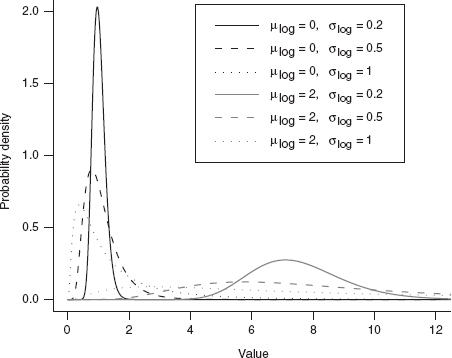
Figure 4.16 Lognormal distribution.
One potentially puzzling aspect of the lognormal distribution is that its mean is not what you might naively expect if you exponentiate a normal distribution with mean μ (i.e., eμ). Because the exponential function is an accelerating function, the mean of the lognormal, ![]() , is greater than eμ (Jensen's inequality). When the variance is small relative to the mean, the mean is approximately equal to eμ, and the lognormal itself looks approximately normal (e.g., solid lines in Figure 4.16, with σ(log) = 0.2). As with the Gamma distribution, the distribution also changes shape as the variance increases, becoming more skewed.
, is greater than eμ (Jensen's inequality). When the variance is small relative to the mean, the mean is approximately equal to eμ, and the lognormal itself looks approximately normal (e.g., solid lines in Figure 4.16, with σ(log) = 0.2). As with the Gamma distribution, the distribution also changes shape as the variance increases, becoming more skewed.
The lognormal is used phenomenologically in some of the same situations where a Gamma distribution also fits: continuous, positive distributions with long tails or variance much greater than the mean (McGill et al., 2006). Like the distinction between a Michaelis-Menten and a saturating exponential function, you may not be able to tell the difference between a lognormal and a Gamma without large amounts of data. Use the one that is more convenient, or that corresponds to a more plausible mechanism for your data.
Examples: sizes or masses of individuals, especially rapidly growing individuals; abundance vs. frequency curves for plant communities.
Summary:
![]()


Figure 4.17 Relationships among probability distributions.
4.6 Extending Simple Distributions: Compounding and Generalizing
What do you do when none of these simple distributions fits your data? You could always explore other distributions. For example, the Weibull distribution (similar to the Gamma distribution in shape: dweibull in ![]() ) generalizes the exponential to allow for survival probabilities that increase or decrease with age (p. 251). The Cauchy distribution (dcauchy in
) generalizes the exponential to allow for survival probabilities that increase or decrease with age (p. 251). The Cauchy distribution (dcauchy in ![]() ), described as fat-tailed because the probability of extreme events (in the tails of the distribution) is very large—larger than for the exponential or normal distributions—can be useful for modeling distributions with many outliers. You can often find useful distributions for your data in modeling papers from your subfield of ecology.
), described as fat-tailed because the probability of extreme events (in the tails of the distribution) is very large—larger than for the exponential or normal distributions—can be useful for modeling distributions with many outliers. You can often find useful distributions for your data in modeling papers from your subfield of ecology.
However, in addition to simply learning more distributions, learning some strategies for generalizing more familiar distributions can also be useful.
4.6.1 Adding Covariates
One obvious strategy is to look for systematic differences within your data that explain the nonstandard shape of the distribution. For example, a bimodal or multimodal distribution (one with two or more peaks, in contrast to most of the distributions discussed above that have a single peak) may make perfect sense once you realize that your data are a collection of objects from different populations with different means. For example, the sizes or masses of sexually dimorphic animals or animals from several different cryptic species would follow bi- or multimodal distributions, respectively. A distribution that isn't multimodal but is more fat-tailed than a normal distribution might indicate systematic variation in a continuous covariate such as nutrient availability, or maternal size, of environmental temperature, of different individuals. If you can measure these covariates, then you may be able to add them to the deterministic part of the model and use standard distributions to describe the variability conditioned on the covariates.
4.6.2 Mixture Models
But what if you can't identify, or measure, systematic differences? You can still extend standard distributions by supposing that your data are really a mixture of observations from different types of individuals, but that you can't observe the (finite) types or (continuous) covariates of individuals. These distributions are called mixture distributions or mixture models. Fitting them to data can be challenging, but they are very flexible.
4.6.2.1 FINITE MIXTURES
Finite mixture models suppose that your observations are drawn from a discrete set of unobserved categories, each of which has its own distribution. Typically all categories have the same type of distribution, such as normal, but with different mean or variance parameters. Finite mixture distributions often fit multimodal data. Finite mixtures are typically parameterized by the parameters of each component of the mixture, plus a set of probabilities or percentages describing the amount of each component. For example, 30% of the organisms (p = 0.3) could be in group 1, normally distributed with mean 1 and standard deviation 2, while 70% (1–p = 0.7) are in group 2, normally distributed with mean 5 and standard deviation 1(Figure 4.18). If the peaks of the distributions are closer together, or their standard deviations are larger so that the distributions overlap, you'll see a broad (and perhaps lumpy) peak rather than two distinct peaks.

Figure 4.18 Finite mixture distribution: 70% Normal(μ = 1, σ = 2), 30% Normal(μ = 5, σ = 1).
Zero-inflated models are a common type of finite mixture model (Inouye, 1999; Martin et al., 2005); we saw a simple example of a zero-inflated binomial at the beginning of this chapter. Zero-inflated models (Figure 4.1) combine a standard discrete probability distribution (e.g., binomial, Poisson, or negative binomial), which typically includes some probability of sampling zero counts even when some individuals are present, with an additional process that can also lead to a zero count (e.g., complete absence of the species or trap failure).
4.6.3 Continuous Mixtures
Continuous mixture distributions, also known as compounded distributions, allow the parameters themselves to vary randomly, drawn from their own distribution. They are a sensible choice for overdispersed data, or for data where you suspect that continuous unobserved covariates may be important. Technically, compounded distributions are the distribution of a sampling distribution S(x, p) with parameter(s) p that vary according to another (typically continuous) distribution P(p). The distribution of the compounded distribution C is C(x) = ∫ S(x, p)P(p)dp. For example, compounding a Poisson distribution by drawing the rate parameter X from a Gamma distribution with shape parameter k (and scale parameter λ/k, to make the mean equal to λ) results in a negative binomial distribution (p. 124). Continuous mixture distributions are growing ever more popular in ecology as ecologists try to account for heterogeneity in their data.
The negative binomial, which could also be called the Gamma-Poisson distribution to highlight its compound origin, is the most common compounded distribution. The beta-binomial is also fairly common: like the negative binomial, it compounds a common discrete distribution (binomial) with its conjugate prior (Beta), resulting in a mathematically simple form that allows for more variability. The lognormal-Poisson is very similar to the negative binomial, except that (as its name suggests) it uses the lognormal instead of the Gamma as a compounding distribution. One technical reason to use the less common lognormal-Poisson is that on the log scale the rate parameter is normally distributed, which simplifies some numerical procedures (Elston et al., 2001).
Clark et al. (1999) used the Student t distribution to model seed dispersal curves. Seeds often disperse fairly uniformly near parental trees but also have a high probability of long dispersal. These two characteristics are incompatible with standard seed dispersal models like the exponential and normal distributions. Clark et al. assumed that the seed dispersal curve represents a compounding of a normal distribution for the dispersal of any one seed with a Gamma distribution of the inverse variance of the distribution of any particular seed (i.e., 1/σ2 ~ Gamma).* This variation in variance accounts for the different distances that different seeds may travel as a function of factors like their size, shape, height on the tree, and the wind speed at the time they are released. Clark et al. used compounding to model these factors as random, unobserved covariates since they are practically impossible to measure for all the individual seeds on a tree or in a forest.
The inverse Gamma-normal model is equivalent to the Student t distribution, which you may recognize from t tests in classical statistics and which statisticians often use as a phenomenological model for fat-tailed distributions. Clark et al. extended the usual one-dimensional t distribution (dt in ![]() ) to the two-dimensional distribution of seeds around a parent and called it the 2Dt distribution. The 2Dt distribution has a scale parameter that determines the mean dispersal distance and a shape parameter p. When p is large the underlying Gamma distribution has a small coefficient of variation and the 2Dt distribution is close to normal; when p = 1 the 2Dt becomes a Cauchy distribution.
) to the two-dimensional distribution of seeds around a parent and called it the 2Dt distribution. The 2Dt distribution has a scale parameter that determines the mean dispersal distance and a shape parameter p. When p is large the underlying Gamma distribution has a small coefficient of variation and the 2Dt distribution is close to normal; when p = 1 the 2Dt becomes a Cauchy distribution.
Generalized distributions are an alternative class of mixture distribution that arises when there is a sampling distribution S(x) for the number of individuals within a cluster and another sampling distribution C(x) for number of clusters in a sampling unit. For example, the distribution of number of eggs per quadrat might be generalized from the distribution of clutches per quadrat and of eggs per clutch. A standard example is the “Poisson-Poisson” or “Neyman Type A” distribution (Pielou, 1977), which assumes a Poisson distribution of clusters with a Poisson distribution of individuals in each cluster.
Figuring out the probability distribution or density formulas for compounded distributions analytically is mathematically challenging (see Bailey (1964) or Pielou (1977) for the gory details), but ![]() can easily generate random numbers from these distributions.
can easily generate random numbers from these distributions.
The key is that ![]() 's functions for generating random distributions (rpois, rbinom, etc.) can take vectors for their parameters. Rather than generate (say) 20 deviates from a binomial distribution with N trials and a fixed per-trial probability p, you can choose 20 deviates with N trials and a vector of 20 different per-trial probabilities p1 to p20. Furthermore, you can generate this vector of parameters from another randomizing function! For example, to generate 20 beta-binomial deviates with N = 10 and the per-trial probabilities drawn from a Beta distribution with a = 2 and b = 1, you could use rbinom(20,prob=rbeta(20,2,1),size=10). (See the R supplement for more detail.)
's functions for generating random distributions (rpois, rbinom, etc.) can take vectors for their parameters. Rather than generate (say) 20 deviates from a binomial distribution with N trials and a fixed per-trial probability p, you can choose 20 deviates with N trials and a vector of 20 different per-trial probabilities p1 to p20. Furthermore, you can generate this vector of parameters from another randomizing function! For example, to generate 20 beta-binomial deviates with N = 10 and the per-trial probabilities drawn from a Beta distribution with a = 2 and b = 1, you could use rbinom(20,prob=rbeta(20,2,1),size=10). (See the R supplement for more detail.)
Compounding and generalizing are powerful ways to extend the range of stochastic ecological models. A good fit to a compounded distribution also suggests that environmental variation is shaping the variation in the population. But be careful: Pielou (1977) demonstrates that for Poisson distributions, every generalized distribution (corresponding to variation in the underlying density) can also be generated by a compound distribution (corresponding to individuals occurring in clusters). She concludes that “the fitting of theoretical frequency distributions to observational data can never by itself suffice to ‘explain' the pattern of a natural population” (p. 123).
4.7 R Supplement
For all of the probability distributions discussed in this chapter (and many more: try help.search(“distribution”)), R can generate random numbers (deviates) drawn from the distribution; compute the cumulative distribution function and the probability distribution function; and compute the quantile function, which gives the x value such that ![]() (the probability that X ≤ x) is a specified value. For example, you can obtain the critical values of the standard normal distribution, ±1.96, with qnorm(0.025) and qnorm(0.975) (Figure 4.19).
(the probability that X ≤ x) is a specified value. For example, you can obtain the critical values of the standard normal distribution, ±1.96, with qnorm(0.025) and qnorm(0.975) (Figure 4.19).
4.7.1 Discrete Distribution
For example, let's explore the (discrete) negative binomial distribution.
First set the random-number seed for consistency so that you get exactly the same results shown here:
![]()
Arbitrarily choose parameters μ = 10 and k = 0.9—since k < 1, this represents a strongly over dispersed population. Remember that ![]() uses size to denote k, because k is mathematically equivalent to the number of failures in the failure-process parameterization.
uses size to denote k, because k is mathematically equivalent to the number of failures in the failure-process parameterization.
![]()
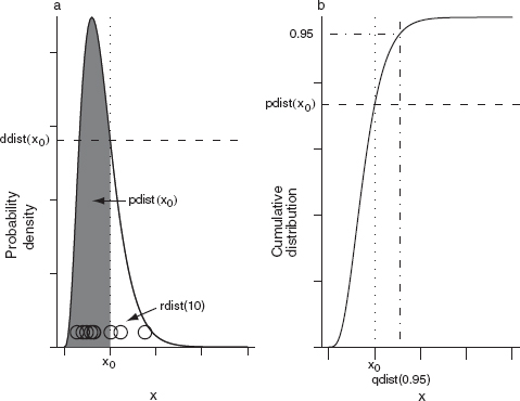
Figure 4.19 R functions for an arbitrary distribution dist, showing density function (ddist), cumulative distribution function (pdist), quantile function (qdist), and random-deviate function (rdist).
Check the first few values:
![]()
Since the negative binomial has no set upper limit, we will just plot the results up to the maximum value sampled:
![]()
The easiest way to plot the results is
![]()
using the levels specification to make sure that all values up to the maximum are included in the plot even when none were sampled in this particular experiment.
If we want the observed probabilities (freq/N) rather than the frequencies:
![]()
Add theoretical values:
![]()
You could plot the deviations with plot(0:maxz,obsprobs-tvals); this gives you some idea how the variability changes with the mean.
Find the probability that x > 30:
![]()
By default R's distribution functions will give you the lower tail of the distribution— the probability that x is less than or equal to some particular value. You could use 1-pnbinom(30,size=0.9,mu=10) to get the upper tail since Prob(x > 30) = 1 — Prob(x < 30), but using lower.tail=FALSE to get the upper tail is more accurate.
What is the upper 95th percentile of the distribution?
![]()
To get the lower and upper 95% confidence limits, you need
![]()
You can also use the random sample z to check that the mean and variance, and the 95th quantile of the sample, agree reasonably well with the theoretical expectations:

4.7.2 Continuous Distribution: Lognormal
Going through the same exercise for the lognormal, a continuous distribution:
![]()
Plot the results:
![]()
Add theoretical values:
![]()
The probability of x > 30:
![]()
95% confidence limits:
![]()
Comparing the theoretical values (p. 137) with the observed values for this random sample:

The difference between the expected and observed variance is fairly large. This is typical: variances of random samples have larger variances, or absolute differences from their theoretical expected values, than means of random samples.
Sometimes it's easier to deal with lognormal data by taking logarithms of the data and comparing them to the normal distribution:
![]()
4.7.3 Mixing and Compounding Distributions
4.7.3.1 FINITE MIXTURE DISTRIBUTIONS
The general recipe for generating samples from finite mixtures is to use a uniform distribution to choose different components of the mixture, then use ifelse to pick values from one distribution or the other. To pick 1000 values from a mixture of normal distributions with the parameters shown in Figure 4.18 (p = 0.3, μ1 = 1, σ1 = 2, μ2 = 5, σ2 = 1):

The probability density of a finite mixture composed of two distributions D1 and D2 in proportions p1 and 1–p1 is P1D1 + (1–P1)D2. We can superimpose the theoretical probability density for the finite mixture above on the histogram:
![]()
The general formula for the probability distribution of a zero-inflated distribution, with an underlying distribution P(x) and a zero-inflation probability of pz, is
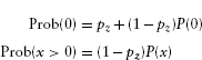
So, for example, we could define a probability distribution for a zero-inflated negative binomial as follows:

(The name, dzinbinom, follows the R convention for a probability distribution function: a d followed by the abbreviated name of the distribution, in this case zinbinom for “zero-inflated negative binomial.”)
The ifelse command checks every element of x to see whether it is zero or not and fills in the appropriate value depending on the answer.
Here's a random deviate generator:

The command runif(n) picks n random values between 0 and 1; the ifelse command compares them with the value of zprob. If an individual value is less than zprob (which happens with probability zprob = pz), then the corresponding random number is zero; otherwise it is a value picked out of the appropriate negative binomial distribution (which may also be zero).
4.7.3.2 COMPOUNDED DISTRIBUTIONS
Start by confirming numerically that a negative binomial distribution is really a compounded Poisson-Gamma distribution. Pick 1000 values out of a Gamma distribution, then use those values as the rate (λ) parameters in random draws from a Poisson distribution:

Establish that a Poisson-lognormal and a Poisson-Gamma (negative binomial) are not very different: pick the Poisson-lognormal with approximately the same mean and variance as the negative binomial just shown.

* N! means N. (N–1). …. 2. 1, and is referred to as “N factorial.”
*If the probability is uniform between a and b on the usual, linear scale (Prob(mass = m) = 1/(b–a)dm), then on the log scale it is Prob(log mass = M) = 1/(b–a)eM dM [if we change variables to log mass M, then dM = d(logm) = 1/m dm, so dm = mdM = eM dM]. Going the other way, a log-uniform assumption gives Prob(mass = m) = 1/(log (b/a)m)dm on the linear scale.
*This value is a probability density, not a probability, so it’s OK for it to be greater than 1: probability density will be explained on p. 116.
*Remember that the 95% confidence limits of the normal distribution are approximately μ±σ.
![]() The kurtosis is sometimes scaled by Var2, or by 3 Var2.
The kurtosis is sometimes scaled by Var2, or by 3 Var2.
*Gelman and Nolan (2002) point out that it is not physically possible to construct a coin that is biased when flipped—although a spinning coin can be biased. Diaconis et al. (2004) even tested a coin made of balsa wood on one side and lead on the other to establish that it was unbiased.
*Beware of the word “overdispersion,” which is sometimes used with an opposite meaning in spatial statistics, where it can mean “more regular than expected from a random distribution of points.” If you took quadrat samples from such an “overdispersed” population, the distribution of counts would have variance less than the mean and would be “underdispersed” in the probability distribution sense (Brown and Bolker, 2004)!
*See p. 131 and the appendix for a description of the Γ (“gamma”) function.
*The lognormal extends our table in another direction—exponential transformation of a known distribution. Other distributions have this property, most notably the extreme-value distribution, which is the log-exponential: if Y is exponentially distributed, then log Y is extreme-value distributed. As its name suggests, the extreme-value distribution occurs mechanistically as the distribution of extreme values (e.g., maxima) of samples of other distributions (Katz et al., 2005).
*This choice of a compounding distribution, which may seem arbitrary, turns out to be mathematically convenient.