6 Likelihood and All That

This chapter presents the basic concepts and methods you need in order to estimate parameters, establish confidence limits, and choose among competing hypotheses and models. It defines likelihood and discusses frequentist, Bayesian, and informationtheoretic inference based on likelihood.

6.1 Introduction

Previous chapters introduced all the ingredients you need to define a model—mathematical functions to describe the deterministic patterns and probability distributions to describe the stochastic patterns—and showed how to use these ingredients to simulate simple ecological systems. The final steps of the modeling process are estimating parameters from data and testing models against each other. You may be wondering by now how you would actually do this.

Estimating the parameters of a model means finding the parameters that make that model fit the data best. To compare among models we have to figure out which one fits the data best, and decide if one or more models fit sufficiently better than the rest that we can declare them the winners. Our goodness-of-fit metrics will be based on the likelihood, the probability of seeing the data we actually collected given a particular model. Depending on the context, “model” could mean either the general form of the model or a specific set of parameter values.

6.2 Parameter Estimation: Single Distributions

Parameter estimation is simplest when we have a a collection of independent data that are drawn from a distribution (e.g., Poisson, binomial, normal), with the same parameters for all observations.^* As an example with discrete data, we will select one particular case out of Vonesh's tadpole predation data (p. 47)—small tadpoles at a density of 10—and estimate the per-trial probability parameter of a binomial distribution (i.e., each individual's probability of being eaten by a predator). As anexample with continuous data, we will introduce a new data set on myxomatosis virus concentration (titer) in experimentally infected rabbits (Myxo in the endbook package; Fenner et al., 1956; Dwyer et al., 1990). Although the titer actually changes systematically over time, we will gloss over that problem for now and pretend that all the measurements are drawn from the same distribution so that we can estimate the parameters of a Gamma distribution that describes the variation in titer among different rabbits.

6.2.1 Maximum Likelihood

We want the maximum likelihood estimates of the parameters—those parameter values that make the observed data most likely to have happened. Since the observations are independent, the joint likelihood of the whole data set is the product of the likelihoods of each individual observation. Since the observations are identically distributed, we can write the likelihood as a product of similar terms. For mathematical convenience, we almost always maximize the logarithm of the likelihood (log-likelihood) instead of the likelihood itself. Since the logarithm is a monotonically increasing function, the maximum log-likelihood estimate is the same as the maximum likelihood estimate. Actually, it is conventional to minimize the negative log-likelihood rather than maximizing the log-likelihood. For continuous probability distributions, we compute the probability density of observing the data rather than the probability itself. Since we are interested in relative (log-)likelihoods, not the absolute probability of observing the data, we can ignore the distinction between the density (P(x)) and the probability (which includes a term for the measurement precision: P(x) dx).

6.2.1.1 TADPOLE PREDATION DATA: BINOMIAL LIKELIHOOD

For a single observation from the binomial distribution (e.g., the number of small tadpoles killed by predators in a single tank at a density of 10), the likelihood that k out of N individuals are eaten as a function of the per capita predation probability p is Prob If we have n observations, each with the same total number of tadpoles N, and the number of tadpoles killed in the. ith observation is ki, then the likelihood is

The log-likelihood is

In R, this would be sum(dbinom(k,size=N,prob=p,log=TRUE)).

Analytical Approach

In this simple case, we can actually solve the problem analytically, by differentiating with respect to p and setting the derivative to zero. Let p be the maximum likelihood estimate, the value of p that satisfies

Since the derivative of a sum equals the sum of the derivatives,

The term log is a constant with respect to p, so its derivative is zero and the first term disappears. Since ki and (N–ki) are constant factors, they come out of the derivatives and the equation becomes

The derivative of log p is 1/p, so the chain rule says the derivative of log (1–p) is Remembering that p is the value of p that satisfies this equation:

So the maximum likelihood estimate, , is just the overall fraction of tadpoles eaten, lumping all the observations together: a total of tadpoles were eaten out of a total of nN tadpoles exposed in all of the observations.

We seem to have gone to a lot of effort to prove the obvious, that the best estimate of the per capita predation probability is the observed frequency of predation. Other simple distributions like the Poisson behave similarly. If we differentiate the likelihood, or the log-likelihood, and solve for the maximum likelihood estimate, we get a sensible answer. For the Poisson, the estimate of the rate parameter is equal to the mean number of counts observed per sample. For the normal distribution, with two parameters μ and σ², we have to compute the partial derivatives (see the appendix) of the likelihood with respect to both parameters and solve the two equations simultaneously The answer is again obvious in hindsight: (the estimate of the mean is the observed mean) and (the estimate of the variance is the variance of the sample).^*

Some simple distributions like the negative binomial, and all the complex problems we will be dealing with hereafter, have no easy analytical solution, so we will have to find the maximum likelihood estimates of the parameters numerically. The point of the algebra here is just to convince you that maximum likelihood estimation makes sense in simple cases.

Numerics

This chapter presents the basic process of computing and maximizing likelihoods (or minimizing negative log-likelihoods) in R; Chapter 7 will go into much more technical detail. First, you need to define a function that calculates the negative log-likelihood for a particular set of parameters. Here's the R code for a binomial negative log-likelihood function:

The dbinom function calculates the binomial likelihood for a specified data set (vector of number of successes) k, probability p, and number of trials N; the log=TRUE option gives the log-probability instead of the probability (more accurately than taking the log of the product of the probabilities); –sum adds the log-likelihoods and changes the sign to compute an overall negative log-likelihood for the data set.

Load the data and extract the subset we plan to work with:

The total number of tadpoles exposed in this subset of the data is 40; (10; in each of 4 trials), 30 of which were eaten by predators, so the maximum likelihood estimate will be = 0.75.

We can use the optim function to numerically optimize (by default, minimizing rather than maximizing) this function. You need to give optim the objective function—the function you want to minimize (binomNLL1 in this case)—and a vector of starting parameters. You can also give it other information, such as a data set, to be passed on to the objective function. The starting parameters don't have to be very accurate (if we had accurate estimates already we wouldn't need optim), but they do have to be reasonable. That's why we spent so much time in Chapters 3 and 4 on eyeballing curves and the method of moments.

fn is the argument that specifies the objective function and par specifies the vector of starting parameters. Using c(p=0.5) names the parameter p—probably not necessary here but very useful for keeping track when you start fitting models with more parameters. The rest of the command specifies other parameters and data and optimization details; Chapter 7 explains why you should use method=“BFGS” for a single-parameter fit.

Check the estimated parameter value and the maximum likelihood—we need to change sign and exponentiate the minimum negative log-likelihood that optim returns to get the maximum log-likelihood:

Because it was computed numerically the answer is almost, but not exactly, equal to the theoretical answer of 0.75.

The mle2 function in the bbmle package provides a “wrapper” for optim that gives prettier output and makes standard tasks easier.^* Unlike optim, which is designed for general-purpose optimization, mle2 assumes that the objective function is a negative log-likelihood function. The names of the arguments are easier to understand: minuslogl instead of fn for the negative log-likelihood function, start instead of par for the starting parameters, and data for additional parameters and data.

The mle2 package has a shortcut for simple likelihood functions. Instead of writing an R function to compute the negative log-likehood, you can specify a formula:

gives exactly the same answer as the previous commands. R assumes that the variable on the left-hand side of the formula is the response variable (k in this case) and that you want to sum the negative log-likelihood of the expression on the right-hand side for all values of the response variable.

Another way to find maximum likelihood estimates for data drawn from most simple distributions—although not for the binomial distribution—is the fitdistr command in the MASS package, which will even guess reasonable starting values for you. However, it works only in the very simple case where none of the parameters of the distribution depend on other covariates.

The estimated value of the per capita predation probability, 0.7499…, is very close to the analytic solution of 0.75. The estimated value of the maximum likelihood (Figure 6.1)is quite small(£ = 5.15 × 10^-4). Thatis, the probability of this particular outcome—5, 7, 9 and 9 out of 10 tadpoles eaten in four replicates—is low.^* In general, however, we will be interested only in the relative likelihoods (or log-likelihoods) of different parameters and models rather than their absolute likelihoods.

Having fitted a model to the data (even a very simple one), it's worth plotting the predictions of the model. In this case the data set is so small (four points) that sampling variability dominates the plot (Figure 6.1b).

6.2.1.2 MYXOMATOSIS DATA: GAMMA LIKELIHOOD

As part of the effort to use myxomatosis as a biocontrol agent against introduced European rabbits in Australia, Fenner and co-workers (1956) studied the virus concentrations (titer) in the skin of rabbits that had been infected with different virus strains. We'll choose a Gamma distribution to model these continuously distributed, positive data. For the sake of illustration, we'll use just the data for one viral strain (grade 1).

Figure 6.1 Binomial-distributed predation. (a) Likelihood curve, on a logarithmic y scale. (b) Best-fit model prediction compared with the data.

The likelihood equation for Gamma-distributed data is hard to maximize analytically, so we'll go straight to a numerical solution. The negative log-likelihood function looks just like the one for binomial data.^*

It's harder to find starting parameters for the Gamma distribution. We can use the method of moments (Chapter 4) to determine reasonable starting values for the scale (= variance/mean) and shape (= mean²/variance = 1/(coefficient of variation)²) parameters.

Since the default parameterization of the Gamma distribution in R uses a rate parameter instead of a scale parameter, I have to make sure to specify the scale parameter explicitly. Or I could use fitdistr from the MASS package:

fitdistr gives slightly different values for the parameters and the likelihood, but not different enough to worry about. A greater possibility for confusion is that fitdistr reports the rate (= 1/scale) instead of the scale parameter.

Figure 6.2 shows the negative log-likelihood (now a negative log-likelihood surface as a function of two parameters, the shape and scale) and the fit of the model to the data (virus titer for grade 1). Since the “true” distribution of the data is hard to visualize (all of the distinct values of virus titer are displayed as jittered values along the bottom axis), I've plotted the nonparametric (kernel) estimate of the probability density in gray for comparison. The Gamma fit is very similar, although it takes account of the lowest point (a virus titer of 4.2) by spreading out slightly rather than allowing the bump in the left-hand tail that the nonparametric density estimate shows. The large shape parameter of the best-fit Gamma distribution (shape = 49.34) indicates that the distribution is nearly symmetrical and approaching normality (Chapter 4). Ironically, in this case the plain old normal distribution actually fits slightly better than the Gamma distribution, despite the fact that we would have said the Gamma was a better model on biological grounds (it doesn't allow virus titer to be negative). However, according to criteria we will discuss later in the chapter, the models are not significantly different and you could choose either on the basis of convenience and appropriateness for the rest of the story you were telling. If we fitted a more skewed distribution, like the damselfish settlement distribution, the Gamma would certainly win over the normal.

6.2.2 Bayesian Analysis

Bayesian estimation also uses the likelihood, but it differs in two ways from maximum likelihood analysis. First, we combine the likelihood with a prior probability distribution in order to determine a posterior probability distribution. Second, we often report the mean of the posterior distribution rather than its mode (which would equal the MLE if we were using a completely uninformative, or “flat,” prior). Unlike the mode, which reflects only local information about the peak of the distribution, the mean incorporates the entire pattern of the distribution, so it can be harder to compute.

Figure 6.2 Likelihood curves for a simple distribution: Gamma-distributed virus titer. Black contours are spaced 200 log-likelihood units apart; gray contours are spaced 20 log-likelihood units apart. In the right-hand plot, the gray line is a kernel density estimate; solid line is the Gamma fit; and dashed line is the normal fit.

6.2.2.1 BINOMIAL DISTRIBUTION: CONJUGATE PRIORS

In the particular case when we have so-called conjugate priors for the distribution of interest, Bayesian estimation is easy. As introduced in Chapter 4, a conjugate prior is a choice of the prior distribution that matches the likelihood model so that the posterior distribution has the same form as the prior distribution. Conjugate priors also allow us to interpret the strength of the prior in simple ways.

For example, the conjugate prior of the binomial likelihood that we used for the tadpole predation data is the Beta distribution. If we pick a Beta prior with shape parameters a and b, and if our data include a total of Σk “successes” (predation events) and nN–Σk “failures” (surviving tadpoles) out of a total of nN “trials” (exposed tadpoles), the posterior distribution is a Beta distribution with shape parameters a + Σk and b + (nN–Σ k). If we interpret a – 1 as the total number of previously observed successes and b – 1 as the number of previously observed failures, then the new distribution just combines the total number of successes and failures in the complete (prior plus current) data set. When a = b = 1, the Beta distribution is flat, corresponding to no prior information (a–1 = b–1 = 0). As a and b increase, the prior distribution gains more information and becomes peaked. We can also see that, as far as a Bayesian is concerned, how we divide our experiments up doesn't matter. Many small experiments, aggregated with successive uses of Bayes' Rule, give the same information as one big experiment (provided of course that there is no variation in per-trial probability among sets of observations, which we have assumed in our statistical model for both the likelihood and the Bayesian analysis).

Figure 6.3 Bayesian priors and posteriors for the tadpole predation data. The scaled likelihood is the normalized likelihood curve, corresponding to the weakest prior possible. Prior(1,1) is weak, corresponding to zero prior samples and leading to a posterior (31,11) that is almost identical to the scaled likelihood curve. Prior(121,81) is strong, corresponding to a previous sample size of 200 trials and leading to a posterior (151,111) that is much closer to the prior than to the scaled likelihood.

We can also examine the effect of different priors on our estimate of the mean (Figure 6.3). If we have no prior information and choose a flat prior with a_prior = b_prior = 1, then our final answer is that the per capita predation probability is distributed as a Beta distribution with shape parameters a = Σ k + 1 = 31, b = nN–Σ k + 1 = 11. The mode of this Beta distribution occurs at (a–1)/(a + b–2) = Σ k/(nN) = 0.75—exactly the same as the maximum likelihood estimate of the per capita predation probability. Its mean is a/(a + b) = 0.738—very slightly shifted toward 0.5 (the mean of our prior distribution) from the MLE. If we wanted a distribution whose mean was equal to the maximum likelihood estimate, we could generate a scaled likelihood by normalizing the likelihood so that it integrated to 1. However, to create the Beta prior that would lead to this posterior distribution we would have to take the limit as a and b go to zero, implying a very peculiar prior distribution with infinite spikes at 0 and 1.

If we had much more prior data—say a set of experiments with a total of (nN)_prior = 200 tadpoles, of which Σ k_prior = 120 were eaten—then the parameters of the prior distribution would be a_prior = 121 and b_prior = 81, the posterior mode would be 0.625, and the posterior mean would be 0.624. In this case both the posterior mode and mean are much closer to the prior values than to the maximum likelihood estimate because the prior information is much stronger than the information we can obtain from the data.

If our data were Poisson, we could use a conjugate prior Gamma distribution with shape α and scale s and interpret the parameters as α = total counts in previous observations and 1/s = number of previous observations. Then if we observed C counts in our data, the posterior would be a Gamma distribution with α' = α + C, 1/s' = 1/s + 1.

The conjugate prior for the mean of a normal distribution, if we know the variance, is also a normal distribution. The posterior mean is an average of the prior mean and the observed mean, weighted by the precisions—the reciprocals of the prior and observed variances. The conjugate prior for the precision, if we know the mean, is the Gamma distribution.

6.2.2.2 GAMMA DISTRIBUTION: MULTIPARAMETER DISTRIBUTIONS AND NONCONJUGATE PRIORS

Unfortunately simple conjugate priors aren't always available, and we often have to resort to numerical integration to evaluate Bayes' Rule. Just plotting the numerator of Bayes' Rule (prior(p) × L(p)) is easy; for anything else, we need to integrate (or use summation to approximate an integral).

In the absence of much prior information for the myxomatosis parameters a (shape) and s (scale), I chose a weak, independent prior distribution:

Bayesians often use the Gamma as a prior distribution for parameters that must be positive (although Gelman (2006) has other suggestions). Using a small shape parameter gives the distribution a large variance (corresponding to little prior information) and means that the distribution will be peaked at small values but is likely to be flat over the range of interest. Finally, the scale is usually set large enough to make the mean of the parameter (= shape ? scale) reasonable. Finally, I made the probabilities of a and s independent, which keeps the form of the prior simple.

As introduced in Chapter 4, the posterior probability is proportional to the prior times the likelihood. To compute the actual posterior probability, we need to divide the numerator Prior(p) × L(p) by its integral to make sure the total area (or volume) under the probability distribution is 1:

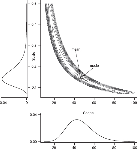
Figure 6.4 Bivariate and marginal posterior distributions for the myxomatosis titer data. Contours are drawn, logarithmically spaced, at probability levels from 0.01 to 10^–10. Posterior distributions are weak and independent, Gamma(shape = 0.1, scale = 10) for scale and Gamma(shape = 0.01, scale = 100) for shape.

Figure 6.4 shows the two-dimensional posterior distribution for the myxomatosis data. As is typical for reasonably large data sets, the probability density is very sharp. The contours shown on the plot illustrate a rapid decrease from a probability density of 0.01 at the mode down to a probability density of 10^–10, and most of the posterior density is even lower than this minimum contour line.

If we want to know the distribution of each parameter individually, we have to calculate its marginal distribution: that is, what is the probability that a or s falls within a particular range, independent of the value of the other variable? To calculate the marginal distribution, we have to integrate (take the expectation) over all possible values of the other parameter:

Figure 6.4 also shows the marginal distributions of a and s.

What if we want to summarize the results still further and give a single value for each parameter (a point estimate) representing our conclusions about the virus titer? Bayesians generally prefer to quote the mean of a parameter (its expected value) rather than the mode (its most probable value). Neither summary statistic is more correct than the other—they give different information about the distribution—but they can lead to radically different inferences about ecological systems (Ludwig, 1996). The differences will be largest when the posterior distribution is asymmetric (the only time the mean can differ from the mode) and when uncertainty is large. In Figure 6.4, the mean and the mode are close together.

To compute mean values for the parameters, we need to compute some more integrals, finding the weighted average of the parameters over the posterior distribution:

(We can also compute these means from the full rather than the marginal distributions: e.g., ^*

R can compute all of these integrals numerically. We can define functions

and use integrate (for one-dimensional integrals) or adapt (in the adapt package; for multidimensional integrals) to do the integration. More crudely, we can approximate the integral by a sum, calculating values of the integrand for discrete values (e.g., s = 0,0.01,…, 10) and then calculating Σ P(s)Δs—this is how I created Figure 6.4.

However, integrating probabilities is tricky for two reasons. (1) Prior probabilities and likelihoods are often tiny for some parameter values, leading to roundoff error; tricks like calculating log probabilities for the prior and likelihood, adding, and then exponentiating can help. (2) You must pick the number and range of points at which to evaluate the integral carefully. Too coarse a grid leads to approximation error, which may be severe if the function has sharp peaks. Too small a range, or the wrong range, can miss important parts of the surface. Large, fine grids are very slow. The numerical integration functions built into R help—you give them a range and they try to evaluate the number of points at which to evaluate the integral—but they can still miss peaks in the function if the initial range is set too large so that their initial grid fails to pick up the peaks. Integrals over more than two dimensions make these problem even worse, since you have to compute a huge number of points to cover a reasonably fine grid. This problem is the first appearance of the curse of dimensionality (Chapter 7).

In practice, brute-force numerical integration is no longer feasible with models with more than about two parameters. The only practical alternatives are Markov chain Monte Carlo approaches, introduced later in this chapter and in more detail in Chapter 7.

For the myxomatosis data, the posterior mode is (a = 47, s = 0.15), close to the maximum likelihood estimate of (a = 49.34, s = 0.14) (the differences are probably caused as much by round-off error as by the effects of the prior). The posterior mean is (a = 45.84, s = 0.16).

6.3 Estimation for More Complex Functions

So far we've estimated the parameters of a single distribution (e.g., X ~ Binom(p) or X ~ Gamma(a, s)). We can easily extend these techniques to more interesting ecological models like the ones simulated in Chapter 5, where the mean or variance parameters of the model vary among groups or depend on covariates.

6.3.1 Maximum Likelihood

6.3.1.1 TADPOLE PREDATION

We can combine deterministic and stochastic functions to calculate likelihoods, just as we did to simulate ecological processes in Chapter 5. For example, suppose tadpole predators have a Holling type II functional response (predation rate = aN/(1 + ahN)), meaning that the per capita predation rate of tadpoles decreases hyperbolically with density (= a/(1 + ahN)). The distribution of the actual number eaten is likely to be binomial with this probability. If N is the number of tadpoles in a tank,

Since the distribution and density functions in R (such as dbinom) operate on vectors just as do the random-deviate functions (such as rbinom) used in Chapter 5, I can translate this model definition directly into R, using a numeric vector p={a, h} for the parameters:

Now we can dig out the data from the functional response experiment of Vonesh and Bolker (2005), which contains the variables Initial (N) and Killed (k). Plotting the data (Figure 2.8) and eyeballing the initial slope and asymptote gives us crude starting estimates of a (initial slope) around 0.5 and h (1/asymptote) around 1/80 = 0.0125.

This optimization gives us parameters (a = 0.526, h = 0.017)—so our starting guesses were pretty good.

To use mle2 for this purpose, you would normally have to rewrite the negative log-likelihood function with the parameters a and h as separate arguments (i.e., function(a,h,p,N,k)). However, mle2 will let you pass the parameters inside a vector as long as you use parnames to attach the names of the parameters to the function.

The answers are very slightly different from the optim results (mle2 uses a different numerical optimizer by default).

As always, we should plot the fit to the data to make sure it is sensible. Figure 6.5a shows the expected number killed (a Holling type II function) and uses the qbinom function to plot the 95% confidence intervals of the binomial distribution.^* One point falls outside of the confidence limits; for 16 points, this isn't surprising (we would expect 1 point out of 20 to fall outside the limits on average), although this point is quite low (5/50, compared to an expectation of 18.3/50—the probability of getting this extreme an outlier is only 2.11 × 10^–5).

Figure 6.5 Maximum-likelihood fits to (a) tadpole predation (Holling type Il/binomial) and (b) myxomatosis (Ricker/Gamma) models.

6.3.1.2 MYXOMATOSIS VIRUS

When we looked at the myxomatosis titer data earlier, we treated it as though it all came from a single distribution. In reality, titers typically change considerably as a function of the time since infection. Following Dwyer et al. (1990), we will fit a Ricker model to the mean titer level. Figure 6.5b shows the data for the grade 1 virus. The Ricker is a good function for fitting data that start from zero, grow to a peak, and then decline, although for the grade 1 virus we have only biological common sense, and the evidence from the other virus grades, to say that the titer would eventually decrease. Grade 1 is so virulent that rabbits die before titer has a chance to drop off. We'll stick with the Gamma distribution for the distribution of titer T at time t, but parameterize it with shape (s) and mean rather than shape and scale parameters (i.e., scale = mean/shape):

Translating this into R is straightforward:

We need initial values, which we can guess knowing from Chapter 3 that a is the initial slope of the Ricker function and 1 /b is the x-location of the peak. Figure 6.5 suggests that a ≈ 1, 1/b ≈ 5. I knew from the previous fit that the shape parameter is large, so I started with shape = 50. When I tried to fit the model with the default optimization method I got a warning that the optimization had not converged, so I used an alternative optimization method, the Nelder-Mead simplex (p. 229).

We could run the same analysis a bit more compactly, without explicitly defining a negative log-likelihood function, using mle2's formula interface:

Specifying data=myxdat lets us use day and titer in the formula instead of myxdat$day and myxdat$titer.

6.3.2 Bayesian Analysis

Extending the tools to use a Bayesian approach is straightforward, although the details are more complicated than maximum likelihood estimation. We can use the same likelihood models (e.g., (6.3.1) for the tadpole predation data or (6.3.2) for myxomatosis). All we have to do to complete the model definition for Bayesian analysis is specify prior probability distributions for the parameters. However, defining the model is not the end of the story. For the binomial model, which has only two parameters, we could proceed more or less as in the Gamma distribution example above (Figure 6.4), calculating the posterior density for many combinations of the parameters and computing integrals to calculate marginal distributions and means. To evaluate integrals for the three-parameter myxomatosis model we would have to integrate the posterior distribution over a three-dimensional grid, which would quickly become impractical.

Markov chain Monte Carlo (MCMC) is a numerical technique that makes Bayesian analysis of more complicated models feasible. BUGS is a program that allows you to run MCMC analyses without doing lots of programming. Here is the BUGS code for the myxomatosis example:

BUGS's modeling language is similar but not identical to R. For example, BUGS requires you to use <– instead of = for assignments.

As you can see, the BUGS model also looks a lot like the likelihood model (6.3.2). Lines 3-5 specify the model (BUGS uses shape and rate parameters to define the Gamma distribution rather than shape and scale parameters: differences in parameterization are some of the most important differences between the BUGS and R languages). Lines 8-10 give the prior distributions for the parameters, all Gamma in this case. The BUGS model is more explicit than (6.3.2)—in particular, you have to put in an explicit for loop to calculate the expected values for each data point—but the broad outlines are the same, even up to using a tilde (˜) to mean “is distributed as.”

You can run BUGS either as a standalone program or from within R, using the R2WinBUGS package as an interface to the WinBUGS program for running BUGS on Windows.^*

You have to specify the names of the data exactly as they are listed in the BUGS model (given above, but stored in a separate text file myxo1.bug):

You also have to specify starting points for multiple chains, which should vary among reasonable values (p. 237), as a list of lists:

(I originally started b at 1.0 for the third chain, but WinBUGS kept giving me an error saying “cannot bracket slice for node a.” By trial and error—eliminating chains and changing parameters—I established that the value of b in chain 3 was the problem.)

Now you can run the model through WinBUGS:

As we will see shortly, you can recover lots of information for a Bayesian analysis from a WinBUGS run—for now, you can use print(myxo1.bugs,digits=4) to see that the estimates of the means, {a = 3.55, b = 0.17, s = 79.9}, are reassuringly close to the maximum likelihood estimates (p. 185).

6.4 Likelihood Surfaces, Profiles, and Confidence Intervals

So far, we've used R and WinBUGS to find point estimates (maximum likelihood estimates or posterior means) automatically, without looking very carefully at the curves and surfaces that describe how the likelihood varies with the parameters. This approach gives little insight when things go wrong with the fitting (as happens all too often). Furthermore, point estimates are useless without measures of uncertainty. We really want to know the uncertainty associated with the parameter estimates, both individually (univariate confidence intervals) and together (bi-or multivariate confidence regions). This section will show how to draw and interpret goodness-of-fit curves (likelihood curves and profiles, Bayesian posterior joint and marginal distributions) and their connections to confidence intervals.

6.4.1 Frequentist Analysis: Likelihood Curves and Profiles

The most basic tool for understanding how likelihood depends on one or more parameters is the likelihood curve or likelihood surface, which is just the likelihood plotted as a function of parameter values (e.g., Figure 6.1). By convention, we plot the negative log-likelihood rather than log-likelihood, so the best estimate is a minimum rather than a maximum. (I sometimes call negative log-likelihood curves badness-of-fit curves, since higher points indicate a poorer fit to the data.) Figure 6.6a shows the negative log-likelihood curve (like Figure 6.1 but upside-down and with a different y axis), indicating the minimum negative log-likelihood (=maximum likelihood) point, and lines showing the upper and lower 95% confidence limits (we'll soon see how these are defined). Every point on a likelihood curve or surface represents a different fit to the data: Figure 6.6b shows the observed distribution of the binomial data along with three separate curves corresponding to the lower estimate (p = 0.6), best fit (p = 0.75), and upper estimate (p = 0.87) of the per capita predation probability.

For models with more than one parameter, we draw likelihood surfaces instead of curves. Figure 6.7 shows the negative log-likelihood surface of the tadpole predation data as a function of attack rate a and handling time h. The minimum is where we found it before, at (a = 0.526, h = 0.017). The likelihood contours are roughly elliptical and are tilted near a 45 degree angle, which means (as we will see) that the estimates of the parameters are correlated. Remember that each point on the likelihood surface corresponds to a fit to the data, which we can (and should) look at in terms of a curve through the actual data values: Figure 6.8 shows the fit of several sets of parameters (the ML estimates, and two other less well-fitting a-h pairs) on the scale of the original data.

Figure 6.6 (a) Negative log-likelihood curve and confidence intervals for binomial-distributed tadpole predation. (b) Comparison of fits to data. Gray vertical bars show proportion of trials with different outcomes; lines and symbols show fits corresponding to different parameters indicated on the curve in (a).

If we want to deal with models with more than two parameters, or if we want to analyze a single parameter at a time, we have to find a way to isolate the effects of one or more parameters while still accounting for the rest. A simple, but usually wrong, way of doing this is to calculate a likelihood slice, fixing the values of all but one parameter (usually at their maximum likelihood estimates) and then calculating the likelihood for a range of values of the focal parameter. The horizontal line in the middle of Figure 6.7 shows a likelihood slice for a, with h held constant at its MLE. Figure 6.9 shows an elevational view, the negative log-likelihood for each value of a. Slices can be useful for visualizing the geometry of a many-parameter likelihood surface near its minimum, but they are statistically misleading because they don't allow the other parameters to vary and thus they don't show the minimum negative log-likelihood achievable for a particular value of the focal parameter.

Instead, we calculate likelihood profiles, which represent “ridgelines” in parameter space showing the minimum negative log-likelihood for particular values of a single parameter. To calculate a likelihood profile for a focal parameter, we have to set the focal parameter in turn to a range of values, and for each value optimize the likelihood with respect to all of the other parameters. The likelihood profile for a in Figure 6.7 runs through the contour lines (such as the confidence regions shown) at the points where the contours run exactly vertical. Think about looking for the minimum along a fixed-a transect (varying h—vertical lines in Figure 6.7); the minimum will occur at a point where the transect is just touching (tangent to) a contour line. Slices are always steeper than profiles (e.g., Figure 6.8), because they don't allow theother parameters to adjust to changes in the focal parameter. Figure 6.9 shows that the fit corresponding to a point on the profile (triangle/dashed line) has a lower value of h (handling time, corresponding to a higher asymptote) that compensates for its enforced lower value of a (attack rate/initial slope), while the equivalent point from the slice (star/dotted line) has the same handling time as the MLE fit, and hence fits the data worse—corresponding to the higher negative log-likelihood in Figure 6.8.

Figure 6.7 Likelihood surface for tadpole predation data, showing univariate and bivariate 95% confidence limits and likelihood profiles for a and h. Darker shades of gray represent higher (i.e., worse) negative log-likelihoods. The solid line shows the 95% bivariate confidence region. Dotted black and gray lines indicate 95% univariate confidence regions. The dash-dotted line and dashed line show likelihood profiles for h and a. The long-dash gray line shows the likelihood slice with varying a and constant h. The black dot indicates the maximum likelihood estimate; the star is an alternate fit along the slice with the same handling time; the triangle is an alternate fit along the likelihood profile for a.

6.4.1.1 THE LIKELIHOOD RATIO TEST

On a negative log-likelihood curve or surface, higher points represent worse fits. The steeper and narrower the valley (i.e., the faster the fit degrades as we move away from the best fit), the more precisely we can estimate the parameters. Since the negative log-likelihood for a set of independent observations is the sum of the individual negative log-likelihoods, adding more data makes likelihood curves steeper. For example, doubling the number of observations will double the negative log-likelihood curve across the board—in particular, doubling the slope of the negative log-likelihood surface.^*

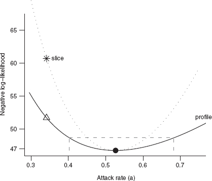
Figure 6.8 Likelihood profile and slice for the tadpole data, for the attack rate parameter a. Gray dashed lines show the negative log-likelihood cutoff and 95% confidence limits for a. Points correspond to parameter combinations marked in Figure 6.6.

It makes sense to determine confidence limits by setting some upper limit on the negative log-likelihood and declaring that any parameters that fit the data at least that well are within the confidence limits. The steeper the likelihood surface, the faster we reach the limit and the narrower are the confidence limits. Since we care only about the relative fit of different models and parameters, the limits should be relative to the maximum log-likelihood (minimum negative log-likelihood).

For example, Edwards (1992) suggested that one could set reasonable confidence regions by including all parameters within 2 log-likelihood units of the maximum log-likelihood, corresponding to all fits that gave likelihoods within a factor of e² ≈ 7.4 of the maximum. However, this approach lacks a frequentist probability interpretation—there is no corresponding p-value. This deficiency may be an advantage, since it makes dogmatic null-hypothesis testing impossible.

Figure 6.9 Fits to tadpole predation data corresponding to the parameter values marked in Figures 6.7 and 6.8.

If you insist on p-values, you can also use differences in log-likelihoods (corresponding to ratios of likelihoods) in a frequentist approach called the Likelihood Ratio Test (LRT). Take some likelihood function and find the overall best (maximum likelihood) value, Now fix some of the parameters (say p₁,…, p_r) to specific values (p₁^*,…p_r^*), and maximize with respect to the remaining parameters to get (r stands for “restricted,” sometimes also called a reduced or nested model). The Likelihood Ratio Test says that twice the negative log of the likelihood ratio, called the deviance, is approximately X² (“chi-squared”) distributed^* with r degrees of freedom.

Figure 6.10 Likelihood profiles and LRT confidence intervals for tadpole predation data.

The log of the likelihood ratio is the difference in the log-likelihoods, so

The definition of the LRT echoes the definition of the likelihood profile, where we fix one parameter and maximize the likelihood/minimize the negative log-likelihood with respect to all the other parameters: r = 1 in the definition above. Thus, for univariate confidence limits we cut off the likelihood profile at where α is our chosen type I error level (e.g., 0.05 or 0.01). The cutoff is a one-tailed test, since we are interested only in differences in likelihood that are larger than expected under the null hypothesis. Figure 6.10 shows the likelihood profiles for a and h, along with the 95% and 99% confidence intervals; you can see how the confidence intervals on the parameters are drawn as vertical lines through the intersection points of the (horizontal) likelihood cutoff levels with the profile.

The 99% confidence intervals have a higher cutoff than the 95% confidence intervals and hence the 99% intervals are wider. The numbers are given in Table 6.1.

R can compute profiles and profile confidence limits automatically. Given an mle2 fit m, profile(m) will compute a likelihood profile and confint(m) will compute profile confidence limits. plot(profile(m2)) will plot the profile, square-root transformed so that a quadratic profile will appear V-shaped (or linear if you specify absVal=FALSE). This transformation makes it easier to see whether the profile is quadratic, since it's easier to see whether a line is straight than it is to see whether it's quadratic. Computing the profile can be slow, so if you want to plot the profile and find confidence limits, or find several different confidence limits, you can save the profile and then use confint on the profile:

TABLE 6.1
Likelihood profile confidence limits

It's also useful to know how to calculate profiles and profile confidence limits yourself, both to understand them better and for the not-so-rare times when the automatic procedures break down. Because profiling requires many separate optimizations, it can fail if your likelihood surface has multiple minima (p. 245) or if the optimization is otherwise finicky. You can try to tune your optimization procedures using the techniques discussed in Chapter 7, but in difficult cases you may have to settle for approximate quadratic confidence intervals (Section 6.5).

To compute profiles by hand, you need to write a new negative log-likelihood function that holds one of the parameters fixed while minimizing the likelihood with respect to the rest. For example, to compute the profile for a (minimizing with respect to h for many values of a), you could use the following reduced negative log-likelihood function (compare this with the full function on p. 183):

The curve drawn by plot(avec,aprof) would look just like the one in Figure 6.10a.

To find the profile confidence limits for a, we have to take one branch of the profile at a time. Starting with the lower branch, the a values below the maximum likelihood estimate:

Finally, use the approx function to calculate the a value for which–L = –:

Now let's go back and look at the bivariate confidence region in Figure 6.7. The 95% bivariate confidence region (solid black line) occurs at negative log-likelihood equal to I've also drawn the univariate region ( contour). That region is not really appropriate for this figure, because it applies to a single parameter at a time, but it illustrates that univariate intervals are smaller than the bivariate confidence region, and that the confidence intervals, like the profiles, are tangent to the univariate confidence region.

The LRT is correct only asymptotically, for large data sets. For small data sets it is an approximation, although one that people use very freely. The other limitation of the LRT that frequently arises, although it is often ignored, is that it applies only when the best estimate of the parameter is away from the edge of its allowable range (Pinheiro and Bates, 2000). For example, if the MLE of the mean parameter of a Poisson distribution λ (which must be ≥ 0) is equal to 0, then the LRT estimate for the upper bound of the confidence limit is not technically correct (see p. 250).

6.4.2 Bayesian Approach: Posterior Distributions and Marginal Distributions

What about the Bayesians? Instead of drawing likelihood curves, Bayesians draw the posterior distribution (proportional to prior × L, e.g., Figure 6.4). Instead of calculating confidence limits using the (frequentist) LRT, they define the credible interval, which is the region in the center of the distribution containing 95% (or some other standard proportion) of the probability of the distribution, bounded by values on either side that have the same probability (or probability density). Technically, the credible interval is the interval [x₁, x₂] such that P(x₁) = P(x₂) and C(x₂)–C(x₁) = 1–α, where P is the probability density and C is the cumulative density. The credible interval is slightly different from the frequentist confidence interval, which is defined as [x₁, x₂] such that C(x₁) = α/2 and C(x₂) = 1–α/2. For empirical samples, use quantile to compute confidence intervals and HPDinterval (“highest posterior density interval”), in the coda package, to compute credible intervals. For theoretical distributions, use the appropriate “q” function (e.g., qnorm) to compute confidence intervals and tcredint, in the emdbook package, to compute credible intervals.

Figure 6.11 shows the posterior distribution for the tadpole predation (from Figure 6.4), along with the 95% credible interval and the lower and upper 2.5% tailsfor comparison. The credible interval is symmetrical in height; the cutoff value on either end of the distribution has the same posterior probability density. The extreme tails are symmetrical in area; the likelihood of extreme values in either direction is the same. The credible interval's height symmetry leads to a uniform probability cutoff: we never include a less probable value on one boundary than on the other. To a Bayesian, this property makes more sense than insisting (as the frequentists do in defining confidence intervals) that the probabilities of extremes in either direction are the same.

Figure 6.11 Bayesian 95% credible interval (gray), and 5% tail areas (hatched), for the tadpole predation data (weak Beta prior: shape = (1,1)).

For multiparameter models, the likelihood surface is analogous to a bivariate or multivariate probability distribution (Figure 6.12). The marginal probability density is the Bayesian analogue of the likelihood profile. Where frequentists use likelihood profiles to make inferences about a single parameter while taking the effects of the other parameters into account, Bayesians use the marginal posterior probability density, the overall probability for a particular value of a focal parameter integrated over all the other parameters. Figure 6.12 shows the 95% credible intervals for the tadpole predation analysis, both bivariate and marginal (univariate). In this case, when the prior is weak and the posterior distribution is reasonably symmetrical, there is little difference between the bivariate 95% confidence region and the bivariate 95% credible interval (Figure 6.12), but Bayesian and frequentist conclusions are not always so similar.

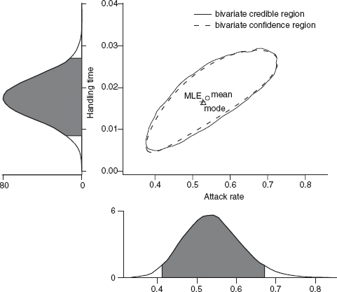
Figure 6.12 Bayesian credible intervals (bivariate and marginal) for tadpole predation analysis.

6.5 Confidence Intervals for Complex Models: Quadratic Approximation

The methods I've discussed so far (calculating likelihood profiles or marginal likelihoods numerically) work fine when you have only two, or maybe three, parameters, but they become impractical for models with many parameters. To calculate a likelihood profile for n parameters, you have to optimize over n–1 parameters for every point in a univariate likelihood profile. If you want to look at the bivari-ate confidence limits of any two parameters, you can't just compute a likelihood surface. To compute a 2D likelihood profile, the analogue of the 1D profiles we calculated previously, you would have to take every combination of the two parameters you're interested in (e.g., a 50 × 50 grid of parameter values) and maximize with respect to all the other n–2 parameters for every point on that surface, and then use the values you've calculated to draw contours. Especially when the likelihood function itself is hard to calculate, this procedure can be extremely tedious.

A powerful, general, but approximate shortcut is to examine the second derivatives of the log-likelihood as a function of the parameters. The second derivatives provide information about the curvature of the surface, which tells us how rapidly the log-likelihood gets worse, which in turn allows us to estimate the confidence intervals. This procedure involves a second level of approximation (like the LRT, becoming more accurate as the number of data points increases), but it can be useful when you run into numerical difficulties calculating the profile confidence limits, or when you want to compute bivariate confidence regions for complex models or more generally explore correlations in high-dimensional parameter spaces.

To motivate this procedure, let's briefly go back to a one-dimensional normal distribution and compute an analytical expression for the profile confidence limits. The likelihood of a set of independent samples from a normal distribution is That means the negative log-likelihood as a function of μ (assuming we know σ) is

where we've lumped the parameter-independent parts of the likelihood into the constant C. We could differentiate this expression with respect to μ and solve for μ when the derivative is zero to show that We could then substitute into (6.5.1) to find the minimum negative log-likelihood. Once we have done this we want to calculate the width of the profile confidence interval c—that is, we want to find the value of c such that

Some slightly nasty algebra leads to

This expression might look familiar: we've just rederived the expression for the confidence limits of the mean! The term is the standard error of the mean; it turns out that the term is the same as the (1–α)/2 quantile for the normal distribution.^* The test uses the quantile of a normal distribution, rather than a Student t distribution, because we have assumed the variance is known.

How does this relate to the second derivative? For the normal distribution, the second derivative of the negative log-likelihood with respect to μ is

So we can rewrite the term in (6.5.3) as the standard deviation of the parameter, which determines the width of the confidence interval, is proportional to the square root of the reciprocal of the curvature (i.e., the second derivative).

While we have derived these conclusions for the normal distribution, they're true for any model if the data set is large enough. In general, for a one-parameter model with parameter p, the width of our confidence region is

where N(α) is the appropriate quantile for the standard normal distribution. This equation gives us a general recipe for finding the confidence region without doing any extra computation, if we know the second derivative of the negative log-likelihood at the maximum likelihood estimate. We can find that second derivative either by calculating it analytically or, when this is too difficult, by calculating it numerically by finite differences. Extending the general rule that the derivative df (p)/dp is approximately (f (p + Δp)–f (p))/Δp:

The hessian=TRUE option in optim tells R to calculate the second derivative in this way; this option is set automatically in mle2.

The same idea works for multiparameter models, but we have to know a little bit more about second derivatives to understand it. A multiparameter likelihood surface has more than one second partial derivative; in fact, it has a matrix of second partial derivatives, called the Hessian. When calculated for a likelihood surface, the negative of the expected value of the Hessian is called the Fisher information; when evaluated at the maximum likelihood estimate, it is the observed information matrix. The second partial derivatives with respect to the same variable twice (e.g., ) represent the curvature of the likelihood surface along a particular axis, while the cross-derivatives, e.g., , describe how the slope in one direction changes as you move along another direction. For example, for the negative log-likelihood –L of the normal distribution with parameters μ and σ, the Hessian is

In the simplest case of a one-parameter model, the Hessian reduces to a single number the curvature of the likelihood curve at the MLE, and the estimated standard deviation of the parameter is just as above.

In some simple two-parameter models such as the normal distribution the parameters are uncorrelated, and the matrix is diagonal:

Figure 6.13 Likelihood ratio and information-matrix confidence limits on the tadpole predation model parameters.

The off-diagonal zeros mean that the slope of the surface in one direction doesn't change as you move in the other direction, and hence the shapes of the likelihood surface in the μ direction and the σ direction are unrelated. In this case we can compute the standard deviations of each parameter independently—they're the inverse square roots of the second partial derivative with respect to each parameter (i.e.,

In general, when the off-diagonal elements are different from zero, we have to invert the matrix numerically, which we can do with solve. For a two-parameter model with parameters a and b we obtain the variance-covariance matrix

where σ_a² and σ_b² are the variances of a and b and σ_ab is the covariance between them; the correlation between the parameters is σ_ab/(σ_aσ_b).

The approximate 80% and 99.5% confidence ellipses calculated in this way are reasonably close to the more accurate profile confidence regions for the tadpole predation data set. The profile region is slightly skewed—it includes more points where d and r are both larger than the maximum likelihood estimate, and fewer where both are smaller—while the approximate ellipse is symmetric around the maximum likelihood estimate.

This method extends to more than two parameters, although it is difficult to draw the analogous pictures in multiple dimensions. The information matrix of a p-parameter model is a p × p matrix. Using solve to invert the information matrix gives the variance-covariance matrix

where σ_i² is the estimated variance of variable i and σ_ij = σ_ji is the estimated covari-ance between variables i and j: the correlation between variables i and j is σ_ij/(σ_iσ_j). For an mle2 fit m, vcov(m) will give the approximate variance-covariance matrix computed in this way and cov2cor(vcov(m)) will scale the variance-covariance matrix by the variances to give a correlation matrix with entries of 1 on the diagonal and parameter correlations as the off-diagonal elements.

The shape of the likelihood surface contains essentially all of the information about the model fit and its uncertainty. For example, a large curvature or steep slope in one direction corresponds to high precision for the estimate of that parameter or combination of parameters. If the curvature is different in different directions (leading to ellipses that are longer in one direction than another), then the data provide unequal amounts of precision for the different estimates. If the contours are oriented vertically or horizontally, then the estimates of the parameters are independent, but if they are diagonal, then the parameter estimates are correlated. If the contours are roughly elliptical (at least near the MLE), then the surface can be described by a quadratic function.

These characteristics also help determine which methods and approximations will work well (Figure 6.14). If the parameters are uncorrelated (i.e., the contours are oriented horizontally and vertically), then you can estimate them separately and still get the correct confidence intervals: the likelihood slice is the same as the profile (Figure 6.14a). If they are correlated, on the other hand, you will need to calculate a profile or invert the information matrix to allow for variation in the other parameters (Figure 6.14b). If the likelihood contours are elliptical—which happens when the likelihood surface has a quadratic shape—the information matrix approximation will work well (Figure 6.14a, b); otherwise, you must use a full profile likelihood to calculate the confidence intervals accurately (Figure 6.14c, d).

You should usually handle nonquadratic and correlated surfaces by computing profile confidence limits, but in extreme cases these characteristics may cause problems for fitting (Chapter 7) and you will have to fall back on the less-accurate quadratic approximations. All other things being equal, smaller confidence regions (i.e., for larger and less noisy data sets and for higher a levels) are more elliptical. Reparameterizing functions can sometimes make the likelihood surface closer to quadratic and decrease correlation between the parameters. For example, one might fit the asymptote and half-maximum of a Michaelis-Menten function rather than the asymptote and initial slope, or fit log-transformed parameters.

Figure 6.14 Varying shapes of likelihood contours and the associated profile confidence intervals, approximate information matrix (quadratic) confidence intervals, and slice intervals. (a) Quadratic contours, no correlation. (b) Quadratic contours, positive correlation. (c) Nonquadratic contours, no correlation. (d) Nonquadratic contours, positive correlation.

6.6 Comparing Models

The last topic for this chapter, a controversial and important one, is model comparison or model selection. Model comparison and selection are closely related to the techniques for estimating confidence regions that we just covered.

Dodd and Silvertown did a series of studies on fir (Abies balsamea) in New York state, exploring the relationships among growth, size, age, competition, and number of cones produced in a given year (Silvertown and Dodd, 1999; Dodd and Silvertown, 2000); see ?Fir in the emdbook package. Figure 6.15 shows the relationship between size (diameter at breast height, DBH) and the total fecundity over the study period, contrasting populations that have experienced wavelike die-offs (“wave”) with those that have not (“nonwave”). A power-law (allometric) dependence of expected fecundity on size allows for increasing fecundity with size while preventing the fecundity from being negative for any parameter values. It also agrees with the general observation in morphometrics that many traits increase as a power function of size. A negative binomial distribution in size around the expected fecundity describes discrete count data with potentially high variance. The resulting model is

Figure 6.15 Fir fecundity as a function of DBH for wave and nonwave populations. Lines show estimates of the model y = a. DBH^b fitted to the populations separately and combined.

We might ask any of these biological/statistical questions:

 

• Does fir fecundity (total number of cones) change (increase) with size (DBH)?

• Do the confidence intervals (credible intervals) of the allometric parameter b include zero (no change)? Do they include one (isometry)?

• Is the allometric parameter b significantly different from (greater than) zero? One?

• Does a model incorporating the allometric parameter fit the data significantly better than a model without an allometric parameter, or equivalently where the allometric parameter is set to zero (µ = a) or one (µ = a. DBH)?

• What is the best model to explain, or predict, fir fecundity? Does it include DBH?

 

Figure 6.15 shows very clearly that fecundity does increase with size. While we might want to know how much it increases (based on the estimation and confidence limits procedures discussed above), any statistical test of the null hypothesis b = 0 would be pro forma. More interesting questions in this case ask whether and how the size-fecundity curve differs in wave and nonwave populations. We can extend the model to allow for differences between the two populations:

where the subscripts i denote different populations—wave (i = w) or nonwave (i = n).

Now our questions become:

 

• Is baseline fecundity the same for small trees in both populations? (Can we reject the null hypothesis a_n = a_w? Do the confidence intervals of a_n — a_w include zero? Does a model with an ≠ aw fit significantly better?)

• Does fecundity increase with DBH at the same rate in both populations? (Can we reject the null hypothesis b_n = b_w? Do the confidence intervals of b_n — b_w include zero? Does a model with bn ≠ bw fit significantly better?)

• Is variability around the mean the same in both populations? (Can we reject the null hypothesis k_n = k_w ? Do the confidence intervals of k_n — k_w include zero? Does a model with kn ≠ kw fit significantly better?)

 

We can boil any of these questions down to the same basic statistical question: for any one of a, b, and k, does a simpler model (with a single parameter for both populations rather than separate parameters for each population) fit adequately? Does adding extra parameters improve the fit sufficiently to justify the additional complexity?

As we will see, these questions one can translate into statistical hypotheses and tests in many ways. While there are stark differences in the assumptions and philosophy behind different statistical approaches, and hot debate over which ones are best, it's worth remembering that in many cases they will all give reasonably consistent answers to the underlying ecological questions. The rest of this introductory section explores some general ideas about model selection. The following sections describe the basics of different approaches, and the final section summarizes the pros and cons of various approaches.

If we ask “does fecundity change with size?” or “do two populations differ?” we know as ecologists that the answer is “yes”—every ecological factor has some impact, and all populations differ in some way. The real questions are, given the data we have, whether we can tell what the differences are, and how we decide which model best explains the data or predicts new results.

Parsimony (sometimes called “Occam's razor”) is a general argument for choosing simpler models even though we know the world is complex. All other things being equal, we should prefer a simpler model to a more complex one—especially when the data don't tell a clear story. Model selection approaches typically go beyond parsimony to say that a more complex model must be not just better than, but a specified amount better than, a simpler model. If the more complex model doesn't exceed a threshold of improvement in fit (we will see below exactly where this threshold comes from), we typically reject it in favor of the simpler model.

Model complexity also affects our predictive ability. Walters and Ludwig (1981) simulated fish population dynamics using a complex age-structured model and showed that when data were realistically sparse and noisy they could best predict future (simulated) dynamics using a simpler non-age-structured model. In other words, even though they knew for sure that juveniles and adults had different mortality rates (because they simulated the data from a model with mortality differences), a model that ignored this distinction gave more accurate predictions. This apparent paradox is an example of the bias-variance trade-off introduced in Chapter 5. As we add more parameters to a model, we necessarily get an increasingly accurate fit to the particular data we have observed (the bias of our predictions decreases), but our precision for predicting future observations decreases as well (the variance of our predictions increases). Data contain a fixed amount of information; as we estimate more and more parameters we spread the data thinner and thinner. Eventually the gain in accuracy from having more details in the model is outweighed by the loss in precision from estimating the effect of each of those details more poorly. In Ludwig and Walters's case, spreading the data out across age classes meant there was not enough data to estimate each age class's dynamics accurately.

Figure 6.16 shows two sets of simulated data generated from a generalized Ricker model, Y ~ Normal((a + bx + cx²)e^—dx). I fitted the first data set with a constant model (y equal to the mean of data), a Ricker model (y = ae^—bx), and the generalized Ricker model. Despite being the true model that generated the data, the generalized Ricker model is overly flexible and adjusts the fit to go through an unusual point at (1.5,0.24). It fits the first data set better than the Ricker (R² = 0.55 for the generalized Ricker vs. _R2= 0.29 for the Ricker). However, the generalized Ricker has overfitted these data. It does poorly when we try to predict a second data set generated from the same underlying model. In the new set of data shown in Figure 6.16, the generalized Ricker fit misses the point near x = 1.5 so badly that it actually fits the data worse than the constant model and has a negative R²! In 500 new simulations, the Ricker prediction was closest to the data 83% of the time, while the generalized Ricker prediction won only 11% of the time; the other 6% of the time, the constant model was best.

6.6.1 Likelihood Ratio Test: Nested Models

How can we tell when we are overfitting real data? We can use the Likelihood Ratio Test, which we used before to find confidence intervals and regions, to choose models in certain cases. A simpler model (with fewer parameters) is nested in another, more complex, model (with more parameters) if the complex model reduces to the simpler model by setting some parameters to particular values (often zero). For example, a constant model, y = a, is nested in the linear model, y = a + bx because setting b = 0 makes the linear model constant. The linear model is nested in turn in the quadratic model, y = a + bx + cx². The linear model is also nested in the Beverton-Holt model, y = ax/(1 + (a/b)x), for b→∞ The Beverton-Holt is in turn nested in the Shepherd model, y = ax/(1 + (a/b)x^d), for d = 1. (The nesting of the linear model in the Beverton-Holt model is clearer if we use the parameterization of the Holling type II model, y = ax/(1 + ahx). The handling time h is equivalent to 1/b in the Beverton-Holt. When h = 0 predators handle prey instantaneously and their per capita consumption rate increases linearly forever as prey densities increase.)

Figure 6.16 Fits to simulated “data” generated with y = (0.4 + 0.1 • x + 2 • x²)e^—x, plus normal error with a = 0.35. Models fitted: constant (y = XX), Ricker (y = ae^—bx), and generalized Ricker (y = (a + bx + cx²)e^—dx). The highlighted point at x ≈ 1.5 drives much of the fit to the original data, and much of the failure to fit new data sets. (a) Data set 1. (b) Data set 2.

Comparisons among different groups can also be framed as a comparison of nested models. If the more complex model has the mean of group 1 equal to a1 and the mean of group 2 equal to a2, then the nested model (both groups equivalent) applies when a1 = a2. It is also common to parameterize this model as a2 = a1 + δ₁₂, where δ₁₂ = a2 — a1, so that the simpler model applies when δ₁₂ = 0. This parameterization works better for model comparisons since testing the hypothesis that the more complex model is better becomes a test of the value of one parameter (δ₁₂ = 0?) rather than a test of the relationship between two parameters (a1 = a2?).^*

To prepare to ask these questions with the fir data, we read in the data, drop NAs, and pull out the variables we want. The fecundity data are not always integers, but a negative binomial model requires integer responses so we round the data.

Using mle2's formula interface is the easiest way to estimate the nested series of models in R. The reduced model (no variation among populations) is

To fit more complex models, use the parameters argument to specify which parameters differ among groups. For example, the argument list(a˜WAVE_NON, b˜WAVE_NON) would allow a and b to have different values for wave and nonwave populations, corresponding to the hypothesis that the populations differ in both a and b but not in variability (a_w ≠ a_n, b_w ≠ b_n, k_w = k_n). The statistical model is Y_i ~ NegBin(ai.; DBH^b_i, k), and the R code is

Here I have used the best-fit parameters of the simpler model as starting parameters for the complex model. Using the best available starting parameters avoids many optimization problems.

mle2's formula interface automatically expands the starting parameter list (which includes only a single value for each of a and b) to include the appropriate number of parameters. mle2 uses default starting parameter values corresponding to equality of all groups, which for this parameterization means that all of the additional parameters for groups other than the first are set to zero.

The formula interface is convenient, but as with likelihood profiles you often encounter situations where you have to know how to do things by hand. Here's an explicit negative log-likelihood model for the model with differences in a and b between groups (we attach the data first for simplicity—don't forget to detach it later):

The first three lines of nbNLL.ab turn the factor WAVE_NON into a numeric code (1 or 2) and use the resulting code as an index to decide which value of a or b to use in predicting the value for each individual. To make k differ by group as well, just change k in the argument list to k.n and k.w and add the line

To simplify the model by making a or b homogeneous, reduce the argument list and eliminate the line of code that specifies the value of the parameter by group.

The only difference between this negative log-likelihood function and the one that mle2 constructs when you use the formula interface is that the mle2-constructed function uses the parameterization {a1, a1 + δ₁₂, whereas our hand-coded function uses {a1,a2} (see p. 205). The former is more convenient for statistical tests, while the latter is more convenient if you want to know the parameter values for each group. To tell mle2 to use the latter parameterization, specify parameters=list(a˜ WAVE_NON-1, b˜WAVE_NON-1). The -1 tells mle2 to fit the model without an intercept, which in this case means that the parameters for each group are specified relative to 0 rather than relative to the parameter value for the first group. When mle2 fills in default starting values for this parameterization, it sets the starting parameters for all groups equal.

The anova function^* performs likelihood ratio tests on a series of nested mle2 fits, automatically calculating the difference in numbers of parameters (denoted by Df for “degrees of freedom”) and deviance and calculating p values:

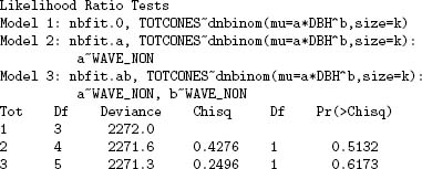
The Likelihood Ratio test can compare any two nested models, testing whether the nesting parameters of the more complex model differ significantly from their null values. Put another way, the LRT tests whether the extra goodness of fit to the data is worth the added complexity of the additional parameters. To use the LRT to compare models, compare the difference in deviances (the more complex model should always have a smaller deviance—if not, check for problems with the optimization) to the critical value of the x² distribution, with degrees of freedom equal to the additional number of parameters in the more complex model. If the difference in deviances is greater than x²_n2—n1 (1 — α), then the more complex model is significantly better at the p = α level. If not, then the additional complexity is not justified.

Choosing among statistical distributions can often be reduced to comparing among nested models. As a reminder, Figure 4.17 (p. 137) shows some of the relationships among common distributions. The most common use of the LRT in this context is to see whether we need to use an overdispersed distribution such as the negative binomial or beta-binomial instead of their lower-variance counterparts (Poisson or binomial). The Poisson distribution is nested in the negative binomial distribution when k → ∞. If we fit a model with a and b varying but using a Poisson distribution instead of a negative binomial, we can then use the LRT to see if adding the overdispersion parameter is justified:

We conclude that negative binomial is clearly justified: the difference in deviance is greater than 4000, compared to a critical value of 3.84! This analysis ignores the nonapplicability of the LRT on the boundary of the allowable parameter space (k →∞ or 1/k = 0; see p. 250), but the evidence is so overwhelming in this case that it doesn't matter.

Models with multiple parameters and multiple groups naturally lead to a web of nested models. Figure 6.17 shows all of the model comparisons for the fir data— even for this relatively simple example there are seven possible models and nine possible series of nested comparisons. In this case the answer is easy, because none of the comparisons is significant according to the LRT (i.e., none of the one-step comparisons differ by more than 3.84). In more complex scenarios deciding which set of comparisons to do first can be quite hard. Two simple options are forward selection (try to add parameters one at a time to the simplest model) and backward selection (try to subtract parameters from the most complex model). Either of these approaches will work, but for comparisons that are close to the edge of statistical significance, or where the effects of the parameters are strongly correlated, you'll often find that you get different answers. Similar problems arise in multiple regression (in fact, in any complex modeling exercise). With too large a set of possibilities, this kind of model selection quickly devolves into data-dredging. You should (1) use common sense and ecological knowledge to isolate the most important comparisons; (2) draw plots of the best candidate fits to try to understand why different models fit the data approximately equally well; and (3) try to rule out differences in variance parameters (k in this case) first. If you can simplify the model in this way it will be more comparable with classical models. If not, something interesting may be happening.

Figure 6.17 Nested hierarchy of models for the fir data. D = deviance.

6.6.2 Information Criteria

One way to avoid a plethora of pairwise model comparisons is to select models based on information criteria, which compare all candidate models at once and do not require nested alternatives. These relatively recent alternatives to Likelihood Ratio Tests are based on the expected distance (quantified in a way that comes from information theory) between a particular model and the “true” model (Burnham and Anderson, 1998, 2002). In practice, all information-theoretic methods reduce to finding the model that minimizes some criterion that is the sum of a term based on the likelihood (usually twice the negative log-likelihood) and a penalty term which is different for different information criteria.

The Akaike Information Criterion, or AIC, is the most widespread information criterion, and is defined as

where L is the log-likelihood and k is the number of parameters in the model.^* As with all information criteria, small values represent better overall fits; adding a parameter with a negligible improvement in fit penalizes the AIC by 2 log-likelihood units. For small sample sizes (n)—such as when n/k < 40 (Burnham and Anderson, 2004, p. 66)—you should use a finite-size correction and apply the AIC_c (“corrected AIC”) instead:

As n grows large, the correction term in (6.6.4) vanishes and the AICc matches the AIC. The AIC_c was originally derived on the basis of linear models with normally distributed errors, so it may apply to a smaller range of models than the AIC—but this is really an open question. Shono (2000) found using simulation studies that the AICc gave accurate answers for typical fisheries data sets, but Richards (2005) suggests that AICc might not perform as well for other kinds of ecological data sets. (I would recommend using AICc for small samples, but being careful with the results if they disagree with the results based on large-sample AIC.)

The second most common information criterion, the Schwarz or Bayesian information criterion (BIC),^† uses a penalty term of (log n)k. When n is greater than e² ≈ 8 observations (so that log n > 2), the BIC is more conservative than the AIC, insisting on a greater improvement in fit before it will accept a more complex model.

Information criteria do not allow frequentist significance tests based on the estimated probability of getting more extreme results in repeated experiments (some statisticians would say this is an advantage). With ICs, you cannot say that there is a statistically significant difference between models; a model with a lower IC is better, but there is no p-value associated with how much better it is.^‡ Instead, there are commonly used rules of thumb: models with ICs less than 2 apart (ΔIC < 2) are more or less equivalent; those with ICs 4-7 apart are clearly distinguishable; and models with ICs more than 10 apart are definitely different. Richards (2005) concurs with these recommendations, but cautions that simply dropping models with ΔAIC > 2 (as some ecologists do) risks discarding useful models.

TABLE 6.2
Results of fir model fits

One big advantage of IC-based approaches is that they do not require nested models.^* You can compare all models to each other simultaneously, rather than stepping through a sometimes confusing sequence of pairwise tests. In IC-based approaches, you simply compute the likelihood and IC for all of the candidate models and rank them in order of increasing IC. The model with the lowest IC is the best fit to the data; those models with ICs within 10 units of the minimum IC are worth considering. As with the LRT, the absolute size of the ICs is unimportant—only the differences in ICs matter.

The AlCtab, AlCctab, and BICtab commands in the bbmle package will compute IC tables from lists of mle fits. Use the options delta=TRUE to get a list of the ΔIC values, weights=TRUE to get AIC weights (see below), sort=TRUE to sort models in order of increasing IC, and nobs to specify the number of observations for BIC or AIC_c. Table 6.2 gives the results for the fir models. All three approaches pick the simplest model as the best model (minimum IC). AIC would keep all models under consideration (ΔIC < 4 for all models), while AIC_c might rule out the most complex model (ΔAIC_c = 4.25), and BIC would definitely rule out complex models where a and b both change (ΔBIC > 10).

ICs can also be useful to choose among stochastic models, which are often not nested. For example, the Gamma, log-normal, and negative binomial models can all describe skewed data, and they all converge to the normal distribution in some limit (Figure 4.17), but there is no easy way to nest them. We can fit the same deterministic model as before (fecundity = a_i. DBH^b_i) with different probability distributions and then use AIC to compare the results.

For each distribution I have to modify the parameters slightly. The lognormal's parameters are the mean and standard deviation of the distribution on the log scale, so I set µ_log = log (a_i. DBH^b) = log a + b log DBH. The Gamma's are shape and scale, with the mean equal to shape. scale, so I set scale = (a. DBH^b)/shape. I also added 0.001 to TOTCONES for the lognormal and Gamma fits because zero values are impossible for the lognormal distribution and for the Gamma distribution with shape > 1, leading to infinite negative log-likelihoods. This problem warns us that a discrete distribution like the negative binomial might make more sense, but a better fit to a continuous distribution might override this concern.

TABLE 6.3
Comparison of stochastic models for fir data

Table 6.3 shows that the negative binomial is best after all.

6.6.3 Bayesian Analyses

Bayesians generally have little interest in formal methods of model selection. Dropping a parameter from a model is often equivalent to testing a null hypothesis that the parameter is exactly zero, and Bayesians consider such point null hypotheses silly. They would describe a parameter's distribution as being concentrated near zero rather than saying its value is exactly zero.^*

Nevertheless, Bayesians do compute the relative probability of different models, in a way that implicitly recognizes the bias-variance trade-off and penalizes more complex models (Kass and Raftery, 1995). Bayesians prefer to make inferences based on averages rather than on most-likely values; for example, they generally use the posterior mean values of parameters rather than the posterior mode. This preference extends to model selection. The marginal likelihood of a model is the probability of observing the data (likelihood), averaged over the prior distribution of the parameters:

where x represents a parameter or set of parameters (if a set, then the integral would be a multiple integral). The marginal likelihood (the average probability of observing a particular data set exactly) is often very small, and we are really interested in the relative probability of different models. If two models have marginal likelihoods and , the Bayes factor is the ratio of the marginal likelihoods, B₁₂ = /, or the odds in favor of model 1.^* If we want to compare several different (not necessarily nested) models, we can look at the pairwise Bayes factors or compute a set of posterior probabilities—assuming that all the models have the same prior probability—by computing the relative values of the marginal likelihoods:

TABLE 6.4
Rules of thumb for Bayes factors

Marginal likelihoods and Bayes factors incorporate an implicit penalty for over-parameterization. When you add more parameters to a model, it can fit better—the maximum likelihood and the maximum posterior probability increase—but at the same time the posterior probability distribution spreads out to cover more less-well-fitting possibilities. Since marginal likelihoods express the mean and not the maximum posterior probability, they will actually decrease when the model becomes too complex.

In principle, using Bayes factors to select the better of two models is simple. If we compare twice the logarithm of the Bayes factors (thus putting them on the deviance scale), the generally accepted rules of thumb for Bayes factors are seen in Table 6.4. That these rules of thumb are similar to those quoted for the AIC is no coincidence. With fairly strong priors, the Bayes factor converges to the AIC instead of the BIC (Kass and Raftery, 1995).

In practice, computing the marginal likelihood for a particular model can be tricky (Congdon, 2003), involving either complicated multidimensional integrals or some kind of stochastic sampling from the prior distribution. One simple approximation is to calculate the harmonic mean of the likelihoods returned from an MCMC run (the harmonic mean is 1/(∑ (1/)/n)). Another, the analogue of the quadratic approximations to the likelihood profile described above, is the Laplace approximation, which combines the posterior mode (the maximum value of prior × likelihood) with information on the curvature of the posterior probability density near the mode.^†

TABLE 6.5
Log Bayes factor approximations for fir models

Most of these approximations improve as the sample size increases: Kass and Raftery (1995) suggest that the Laplace approximation requires at least 5 times as many samples as parameters, and that the other approximations should be reasonable with 20 times as many samples as parameters. How do these approximations compare for the fir data set, with 242 data points and up to 6 parameters? Table 6.5 shows that the different approximations of the Bayes factor do differ considerably, but the only qualitative difference among them according to the rules of thumb is that the evidence supporting the null model (all parameters equal) over the model with different a and b parameters is “positive” according to the harmonic mean and “strong” according to the Laplace approximation and BIC.

A more recent criterion, conveniently built into WinBUGS, is the DIC, or deviance information criterion, which was designed particularly for models containing random effects where even specifying the number of parameters is challenging (see Chapter 10). To compute DIC, start by calculating , the average of the deviance over the posterior distribution (as contrasted with the marginal likelihood, which is the average over the prior distribution), and , which is the deviance calculated at the posterior mean parameters. Then use these two values to estimate an effective number of parameters pD = — ; the more spread out the posterior distribution, the bigger the difference between the deviance of the mean parameters and the mean deviance, and the larger the effective number of parameters. Finally, as with AIC and BIC, use this effective number of parameters as a penalty term on the goodness of fit (defined in this case as the deviance at the mean parameters ): DIC= + 2_pD. As with all information criteria, lower values of DIC indicate a better model. The rules of thumb are similar too: differences in DIC from 5 to 10 indicate that one model is clearly better, whereas models with difference in DIC > 10 probably don't need to be considered further (Spiegelhalter et al., 2002).

Two important cautions about the DIC are:

 

• If the model contains random effects (see Chapter 9), the DIC focuses on the random effects. In the fir tree case, because of a peculiarity of BUGS, we had to parameterize the negative binomial model by assuming that each tree's fecundity is a Poisson variable with a different, Gamma-distributed rate. Since DIC focuses on random effects, it reports the effective number of parameters as > 200 (it takes a lot of information to describe the variation in rates), and the effective number of parameters for the most complex model is actually slightly smaller than for the simpler model, because the variation in the rates is slightly lower. This drop in effective model size gives the most complex model the lowest DIC. However, the range of DICsis very small—from 1709.2 to 1710.9—so the DIC is really telling us that the models can't be well distinguished.

• DIC is convenient, and so it is likely to become established as the standard “canned” method of model comparison in Bayesian statistics. It has already begun to appear in ecological journals (Jonsen et al., 2003; McCarthy and Parris, 2004; Morales et al., 2004; Okuyama and Bolker, 2005; Parris, 2006; Vesk, 2006), but statisticians continue to debate its exact meaning and appropriateness (both Spiegelhalter et al. (2002) and Celeux et al. (2006) are accompanied by lively discussions).

 

The bottom line on Bayesian model selection is that, despite the conceptual simplicity of the Bayes factor (giving the “average” quality of fit to the data, and automatically incorporating a penalty for overfitting), it is difficult to calculate and so is likely to be superseded by the convenient DIC. You should exercise the same care with DIC as you would with any canned model selection procedure.

6.6.4 Model Weighting and Averaging

Bayesians themselves would say that you should not simply select one model. Taking the best model and ignoring the rest is equivalent to assigning a probability of 1.0 to the best and 0.0 to the rest. Model averaging methods take the average of the predictions of different models, weighted by the probability of the models or by some other index.

Bayesian model averaging simply takes the probabilities based on the marginal likelihoods or the BIC: the posterior probabilities of a set of models, if they all have equal prior probabilities, are the marginal likelihoods (or BICs) divided by the sum of the marginal likelihoods (or BICs).^* If a set of models have BIC values, relative to the best one, of ΔB_i (where ΔB_i = BIC_i — min (BIC)), then the approximate posterior probabilities of the models, assuming all the prior probabilities are equal, are

To make a weighted prediction, use the posterior probabilities to combine the predictions of the different models (say C₁, C₂,…, C_n):

Of course, you can do the same with marginal likelihoods.

Burnham and Anderson (1998, 2002) have also promoted model averaging, in their case based on AIC weights. The AIC weights are analogous to the probabilities calculated from the relative BIC values, but with AIC values substituted for BIC values in (6.6.7). AIC weights have no probability interpretation, but they can be used in model averaging.^*

Even if you don't do formal model averaging, AIC or BIC weights are a useful way of getting a feel for the relative goodness-of-fit of different models.

6.6.5 Model Criticism and Goodness-of-Fit Tests

If the best model is a poor fit to the data, then none of the machinery of model selection and averaging makes sense. You should always check that your model gives a reasonable fit to the data. Goodness-of-fit testing may remind you of the classical Pearson chi-square statistic, adding up ((expected–observed)²/expected) for all of your data to test whether the variance around the model predictions is greater than expected. However, the chi-square test works only for simple count data where the answers fall in discrete groups. If your data are continuous, or if you are using an overdispersed distribution such as the negative binomial, then your model contains a parameter describing the variance and the chi-square test is no longer useful.^†

In practice, model criticism (a more generic term than goodness-of-fit testing) is simply common sense. Are the predictions reasonable? Are there consistent deviations from the estimates or unexplained outliers? Start with a simple graph of the predictions of the model (Figure 6.15), to see whether the deterministic component of the model works well.

Plots of predicted vs. actual data (Figure 6.18), or of the residuals (actual–predicted) from a model can sometimes be useful. You have already had to figure out how to calculate the predicted values in order to write a likelihood function. Take these values and plot them against the corresponding data points, then use abline(a=0,b=1) to add a predicted = actual line to the plot. However, while the predicted-vs.-actual plot can identify outliers, it really gives a consistency check rather than providing any new information. Ideally, the scatter around the predicted = actual line will be small—in which case the deterministic component of the model explains most of the variation in the data, so that the model is precise as well as accurate—and therefore useful for prediction. Remember, though, that a reasonable amount of unexplained variability does not necessarily mean that the model fits badly or is not useful; it just means it can't make precise predictions.^‡ Model criticism is more concerned with systematic deviations that suggest that the form of the model itself is wrong.

Figure 6.18 Predicted vs. actual cones for the fir data, on a logarithmic scale.

Examining the goodness of fit of the stochastic part of a model is harder. If the model contains only discrete groups (factors), you can divide the data into those groups and overlay the observed distribution (described by a histogram or density plot) with the predicted distribution. If it contains continuous covariates, you may have to break the data up into discrete subsets in order to compare the predicted and observed distributions (Figure 6.19).

6.6.6 Model Selection: Comparisons and Conclusions

Deciding what models to use and how to use them is fundamentally difficult. In one form or another, this debate goes all the way back to the early Bayesian/frequentist divide. While statisticians have come a long way in exploring the possible approaches and (to some extent) in providing practical recipes for applying them, we still do not have—and never will have—a single best method.

 

•   Hypothesis testing based on the Likelihood Ratio test is well-established, widely used, and simple to implement. At times when we really do want a yes-or-no answer about whether some ecological factor is affecting the system in a way that is distinguishable from randomness, the LRT is appropriate. The LRT becomes unwieldy when there are many possibly interacting factors—one has to choose a path through the nested hierarchy of factors (Figure 6.17). Analogous problems in multiple regression analysis led to stepwise model-building approaches, which are widely used by researchers but widely dismissed by statisticians because they encourage data-dredging and because the results depend on the exact thresholds used to include or exclude factors from the model (Whittingham et al., 2006).

Figure 6.19 Goodness-of-fit checking for the fir model. Panels break data up by wave/ non-wave (rows) and DBH (columns) and plot the density of points for each category along with the predicted negative binomial distribution (gray) for the mean DBH value in the category.

If you do find yourself with seemingly inconsistent results from an LRT analysis (e.g., if some parameters are significant only when other parameters are included in the model; Lindsey (1999b) calls these incompatible results), examine your data carefully to understand how the fit changes with different sets of parameters. If two parameters explain essentially the same patterns in the data (e.g., if you are using strongly correlated predictors like soil moisture and precipitation), then whichever enters the model first will be selected. On the other hand, the effects of nitrogen availability might be visible only after the effects of soil moisture are accounted for—in this case, nitrogen would be significant only if soil moisture were in the model already. These kinds of interactions are challenging, but handled properly they tell you more about what's going on in your data.

•   Information theoretic (AIC-based) approaches are also well-established and practical. They neatly avoid the problem of pairwise testing, the need for nested models, and the philosophical issues associated with null hypothesis testing—rather than asking about the probability of a more extreme outcome, they simply try to identify the model with the best predictive ability. They can be used for model averaging, taking the predictions of all reasonable models into account, as well as for model testing. However, AIC-based approaches can also be abused (Guthery et al., 2005). Precisely because of their ease of use, they have led some ecologists down the path of data-dredging and thoughtless model selection (against the warnings of Burnham and Anderson, AIC's main proponents in ecology).

AIC-based analyses make decisions based on rules of thumb about ΔAIC values or AIC weights, which are in turn based on extensive simulation analysis. The results do not have probabilistic or “statistical significance” interpretations (which may be a good thing). In some theoretical situations (i.e., when sample sizes grow large but the set of candidate models remains fixed), AIC is known to “overfit” data by choosing an inappropriately complex model. Researchers hotly debate the practical relevance of this issue (Spiegelhalter et al., 2002; Burnham and Anderson, 2004; Link and Barker, 2006).

•   Bayesian (marginal likelihood, BIC, DIC) approaches are philosophically satisfying since they allow us to state results in terms of posterior probabilities of different models. The selection criteria (posterior probabilities) depend on the number of the parameters and on the sample size, which seems sensible. However, Bayesian approaches are also challenging to apply. Marginal likelihood is hard to calculate in a stable way; BIC is an approximation to the marginal likelihood that applies when sample sizes are large and the priors are vague (AIC is similarly an approximation to a marginal likelihood with a fairly strongly informative prior). For reasonable sample sizes, BIC will be more conservative than AIC; whether this conservatism is appropriate is still a matter of deep contention. Some researchers cannot accept a method that gives the wrong answer in the limit of large amounts of data, while others are more concerned with the performance of the method in the more realistic, data-limited case.^*

DIC is promising but continues to be controversial among statisticians. According to Spiegelhalter et al. (2002, p. 613), it is “a Bayesian analogue of AIC, with a similar justification but wider applicability.” It is similar to AIC in its large-sample behavior. DIC is likely to become increasingly popular among ecologists since it is implemented in WinBUGS. Bayesian approaches are also sensitive to the priors used: one may not be able to get away with the common practice of setting a vague prior and forgetting about it.

 

Should we use formal rules to do model selection (or averaging) at all? Most Bayesians would say that all possible model components really exist in the world, and we ought not throw components away just because they fall below some arbitrary threshold criterion. Gelman et al., (1996) prefer to formulate selection problems as estimating a continuous parameter rather than selecting from discrete choices. Bayesians do recognize the fundamental trade-off between bias and variance, but in general they use less formal methods (such as checking whether the marginal posterior distribution has a peak, indicating that the model component is not just adding noise to the model) to decide what components to include.

A second, more intuitive argument usually comes from biologists, who are unhappy when their favorite bit of biology is dropped from a model even though they know that mechanism operates in nature. If you want to evaluate the effects of age structure (or spatial structure, or genetic structure) on population dynamics, you have to include it in the model even if a formal model selection procedure tells you to leave it out (Hilborn and Mangel, 1997, p. 261). What the model selection criterion is warning you, however, is that you may be basing your conclusions on dangerously little information.

A third argument often comes from conservationists who are concerned that adding a biologically relevant but statistically insignificant term to the model changes the predicted dynamics of a species, often for the worse. This is a real problem, but it is also sometimes used dishonestly. Adding complexity to a model often makes its dynamics less stable, and if you're looking to bolster an argument that a species is in trouble and needs to be protected, you'll favor results that show the species is in trouble. How often do we see conservationists arguing for more realistic biological models that suggest that a species is in no real danger and needs no protection? (On the flip side, how often do we see developers arguing that we should sample more thoroughly to make absolutely sure that there are no endangered species on a tract of land before starting construction?)

There are rules of thumb and procedures for model selection, but they don't settle the fundamental questions of model selection. Is parsimony really the most important thing? Is it OK to add more complexity to the model if you're interested in a particular biological mechanism, even if the data don't appear to support it? In the end you have to learn all the rules, but also know when to bend them—and when you do bend them, give a clear justification. The variety of model selection approaches opens a new avenue for data-dredging, by trying many different procedures and choosing the one that gives you the answers you want.

6.7 Conclusion

This chapter has covered an enormous amount of material, starting from the basic ideas of likelihood and maximum likelihood estimation, discussing various ways of estimating confidence intervals, and tackling the contentious issue of hypothesis testing and model selection. The two big ideas to take away are: (1) The geometry of the likelihood surface or posterior probability distribution—where it peaks and how the distribution falls off around the peak—contains essentially all the information you need to estimate parameters and confidence intervals. (2) Deciding which models to use for inference is challenging and cannot be reduced to a simple recipe. Different approaches correspond to different questions about the data.

---

^* In statistical jargon, such data are called independent and identically distributed (iid).

^* The symbol ∏ denotes a product, like Σ but for multiplication.

^* Maximum likelihood estimation gives a biased estimate of the variance, dividing the sum of squares by n instead of n–1.

^* Why mle2? There is an mle function in the stats4 package that comes with R, but I added some features—and then renamed it to avoid confusion with the original R function.

^* I randomly simulated 1000 samples of four values drawn from the binomial distribution with p = 0.75, N = 10. The maximum likelihood was smaller than the observed value given in the text 12.4% of the time (or 54% of the time if we keep only the samples where 30/40 tadpoles were eaten). Thus this likelihood, although small, is not significantly lower than would be expected by chance.

We could also use a log-normal distribution or (since the minimum values are far from zero and the distributions are reasonably symmetric) a normal distribution.

^* optim insists that you specify all of the parameters packed into a single numeric vector in your negative log-likelihood function. mle prefers the parameters as a list. mle2 will accept either a list, or, if you use parnames to specify the parameter names, a numeric vector (p. 183).

Because the estimates of the shape and scale are very strongly correlated in this case, I ended up having to tweak the starting conditions slightly away from the method of moments estimates, to {45.8,0.151}.

^* The means of the marginal distributions are the same as the mean of the full distribution. Confusingly, the modes of the marginal distributions are not the same as the mode of the full distribution.

^* These confidence limits, sometimes called plug-in estimates, ignore the uncertainty in the parameters.

^* WinBUGS runs on Windows and on Intel machines under Linux or MacOS (using Wine or Crossover Office). Chapter 7 gives more details.

^* Doubling the sample size also typically doubles the minimum negative log-likelihood as well, which may seem odd—why would adding more data worsen the fit of the model?—until you remember that we're not really interested in the probability of a particular set of data, just the relative likelihood of different models and parameters. The probability of flipping a fair coin (p = 0.5) twice and getting one head and one tail is 0.5. The probability of flipping the same coin 1000 times and getting 500 heads and 500 tails is only 0.025; that doesn't mean that we should reject the hypothesis that the coin is fair.

^* You may associate the X² distribution with contingency table analysis, chisq.test in R, but it is a distribution that appears much more broadly in statistics.

Here's a heuristic explanation: you can prove that the distribution of the maximum likelihood estimate is asymptotically normally distributed (i.e., with sufficiently large sample sizes). You can also show, by Taylor expanding, that the log-likelihood surface is quadratic, with curvature determined by the variances of the parameters. If we are restricting r parameters, then we are moving away from the maximum likelihood of the more complex model in r directions, by a normally distributed amount θ_i in each direction. Since the log-likelihood surface is quadratic, the drop in the negative log-likelihood is Since the θ_i values (likelihood estimates of each parameter) are each normally distributed, the sum of squares of r of them is X² distributed with r degrees of freedom. This explanation is necessarily crude; for the real derivation, see Kendall and Stuart (1979).

^*Try sqrt(qchisq(0.95,1)) and qnorm(0.975) in R to test this idea; use 0.975 instead of 0.95 in the second expression because this procedure involves a two-tailed test on the normal distribution but a one-tailed test on the X² distribution, because X² is the distribution of a squared normal deviate.

^* We can also interpret these parameterizations geometrically. In (a₁,a₂) parameter space, we're testing to see whether the best fit falls on the line through the origin a1 = a2; in (a1, S12) parameter space, we're testing whether the best fit lies on the line S12 = 0. To explore further how different parameterizations relate to testing different hypotheses, look for the topic of contrasts in statistical models (Crawley, 2002; Venables and Ripley, 2002).

^* Why anova? The corresponding series of tests for a simple linear model with categorical predictors is an analysis of variance (Chapter 9).

^* Where does the magic penalty term 2k come from? AIC is the expected value of the Kullback-Leibler distance J f (x) log (f (x)/g(x0)) dx: in words, the K — L distance is the log ratio between f (x), the likelihood of the true model and parameters, and g(x0), the likelihood of a candidate model evaluated at its best parameters, averaged over the true distribution of the data. Separating terms and dropping constants that don't involve g(x0), we get £[— log g(x0)]. We don't know the true MLE x0, only the observed MLE x, sowe take another expectation: £[£[— logg(x)]]. Taylor expanding — logg(x) around x0, the expectation of the linear term drops out, leaving the constant and quadratic terms: £[£[— log g(x) — j(x — x)^TV(x — x)]]. V is the matrix of second derivatives of the log-likelihood (the information matrix): — V^—1 ≈ E, the variance-covariance matrix of the parameters. By definition, £[(x — x)^T(x — x)] also equals E. After more math, we get — logg(x) + trace(E^—1E), where the trace is the sum of the diagonal elements of a matrix. Since a matrix times its inverse is the identity matrix, this becomes — log g(x) + k, where k is the size of the matrix—which equals the number of parameters. Doubling this expression so that the first term is the deviance (—2L) gives —2L + 2k. For more information, see Ripley (2004) or Chapter 7 of Burnham and Anderson (2002).

^† While the BIC is derived from a Bayesian argument, it is not inherently a Bayesian technique. It is also not how most Bayesians would compare models (Section 6.6.3).

^‡ Burnham and Anderson (2002, p. 84) recommend avoiding the word “significant” in conjunction with AIC-based model selection; no matter how carefully you phrase your conclusions, some readers will impose a frequentist hypothesis-testing interpretation.

^* Although some, such as Ripley (2004), disagree.

^* Although they might consider testing a hypothesis about whether a parameter is small (i.e., whether its absolute value is below some threshold (Gelman and Tuerlinckx, 2000)).

^* The Bayes factor is based on assuming equal prior probabilities (p1 = p2 = 0.5) for both models.

^† The Laplace approximation is

where d is the number of parameters, |V| is the determinant of the variance-covariance matrix estimated from the Hessian at the posterior mode, and Post_max is the height of the posterior mode.

^* Equal prior probabilities for all the models usually makes sense, although one does face some of the questions about equal priors raised in Chapter 4; for example, should all of the models incorporating differences between groups in the fir example be treated as subsets of a single model?

^* Akaike weights are widely and incorrectly presented as “the probability that model i is the best model for the observed data, given the candidate set of models” (Mazerolle, 2004; Johnson and Omland, 2004). Burnham and Anderson (2004) are more careful: they say that the AIC weights “are interpreted as probabilities…” (emphasis added), but it is clearly a slippery slope. Taking AIC weights as actual probabilities is trying to have one's cake and eat it too; the only rigorous way to compute such probabilities of models is to use Bayesian inference, with its associated complexities (Link and Barker, 2006).

^† Much of the protocol that Burnham and Anderson (2002) have developed for working with AIC concerns testing and correcting for overdispersion— in their notation. These overdispersion corrections are relevant only when your model uses a simple count distribution such as binomial or Poisson.

^‡ People who are familiar with classical statistical approaches would often like to compute an R² statistic (proportion variance explained) for a model. Unfortunately, “despite various analogs for categorical response models, no proposed measure is as widely useful as R and R²“ (Agresti, 2002, p. 390).

^* Lindsey (1999b) suggests an adjustable penalty term that depends on the sample size and may fall somewhere between the AIC and BIC criteria, but he gives little guidance on choosing such a penalty.