7 Optimization and All That

This chapter explores the technical methods required to find the quantities discussed in the previous chapter (maximum likelihood estimates, posterior means, and profile confidence limits). The first section covers methods of numerical optimization for finding MLEs and Bayesian posterior modes, the second section introduces Markov chain Monte Carlo, a general algorithm for finding posterior means and credible intervals, and the third section discusses methods for finding confidence intervals for quantities that are not parameters of a given model.

7.1 Introduction

Now we can think about the nitty-gritty details of fitting models to data. Remember that we're trying to find the parameters that give the maximum likelihood for the comparison between the fitted model(s) and the data. (From now on I will discuss the problem in terms of finding the minimum negative log-likelihood, although all the methods apply to finding maxima as well.) The first section focuses on methods for finding minima of curves and surfaces. These methods apply whether we are looking for maximum likelihood estimates, profile confidence limits, or Bayesian posterior modes (which are an important starting point in Bayesian analyses (Gelman et al., 1996)). I will discuss the basic properties of a few common numerical minimization algorithms (most of which are built into R), and their strengths and weaknesses. Many of these methods are discussed in more detail by Press et al. (1994). The second section introduces Markov chain Monte Carlo methods, which are the foundation of modern Bayesian analysis. MCMC methods feel a little bit like magic, but they follow simple rules that are not too hard to understand. The last section tackles a more specific but very common problem, that of finding confidence limits on a quantity that is not a parameter of the model being fitted. There are many different ways to tackle this problem, varying in accuracy and difficulty. Having several of these techniques in your toolbox is useful, and learning about them also helps you gain a deeper understanding of the shapes of likelihood and posterior probability surfaces.

7.2 Fitting Methods

7.2.1 Brute Force/Direct Search

The simplest way to find a maximum (minimum) is to evaluate the function for a wide range of parameter values and see which one gives the best answer. In R, you would make up a vector of parameter values to try (perhaps a vector for each of several parameters); use sapply (for a single parameter) or for loops to calculate and save the negative log-likelihood (or posterior log-likelihood) for each value; then use which(x==min(x)) (or which.min(x)) to see which parameter values gave the minimum. (You may be able to use outer to evaluate a matrix of all combinations of two parameters, but you have to be careful to use a vectorized likelihood function.)

The big problem with direct search is speed, or lack of it: the resolution of your answer is limited by the resolution (grid size) and range of your search, and the time needed is the product of the resolution and the range. Suppose you try all values between p_lower and p_upper with a resolution Δ p (e.g., from 0 to 10 by steps of 0.1). Figure 7.1 shows a made-up example—somewhat pathological, but not much worse than some real likelihood surfaces I've tried to fit. Obviously, the point you're looking for must fall in the range you're sampling: sampling grid 2 in the figure misses the real minimum by looking at too small a range.

You can also miss a sharp, narrow minimum, even if you sample the right range, by using too large a Δp—sampling grid 3 in Figure 7.1. There are no simple rules for determining the range and Δp to use. You must know the ecological meaning of your parameters well enough that you can guess at an appropriate order of magnitude to start with. For small numbers of parameters you can draw curves or contours of your results to double-check that nothing looks funny, but for larger models it's difficult to draw the appropriate surfaces.

Furthermore, even if you use an appropriate sampling grid, you will know the answer only to within Δp. If you use a smaller Δp, you multiply the number of values you have to evaluate. A good general strategy for direct search is to start with a fairly coarse grid (although not as coarse as sampling grid 3 in Figure 7.1), find the subregion that contains the minimum, and then “zoom in” on that region by making both the range and Δp smaller, as in sampling grid 4. You can often achieve fairly good results this way, but almost always less efficiently than with one of the more sophisticated approaches covered in the rest of the chapter.

The advantages of direct search are (1) it's simple and (2) it's so dumb that it's hard to fool: provided you use a reasonable range and Δp, it won't be led astray by features like multiple minima or discontinuities that will confuse other, more sophisticated approaches. The real problem with direct search is that it's slow because it takes no advantage of the geometry of the surface. If it takes more than a few seconds to evaluate the likelihood for a particular set of parameters, or if you have many parameters (which leads to many many combinations of parameters to evaluate), direct search may not be feasible.

For example, to do direct search on the parameters of the Gamma-distributed myxomatosis data, we need to set the range and grid size for shape and scale. In Chapter 6, we used the method of moments to determine starting values of shape (53.9) and scale (0.13). We'll try shape parameters from 10 to 100 with Δshape = 1, and scale parameters from 0.01 to 0.3 with Δscale = 0.01.

Figure 7.1 Direct search grids for a hypothetical negative log-likelihood function. Grids 1 and 4 will eventually find the correct minimum (open point). Grids 2 and 3 will miss it, finding the false minimum (closed point) instead. Grid 2 misses because its range is too small; grid 3 misses because its resolution is too small.

Using the gammaNLLl negative log-likelihood function from p. 175:

Draw the contour plot:

Or you can do this more automatically with the curve3d function from the emdbook package:

The gridsearch2d function (also in emdbook) will let you zoom in on a negative log-likelihood surface:

7.2.2 Derivative-Based Methods

The opposite extreme from direct search is to make strong assumptions about the geometry of the likelihood surface: typically, that it is smooth (continuous with continuous first and second derivatives) and has only one minimum. At this minimum point the gradient, the vector of the derivatives of the surface with respect to each parameter, is a vector of all zeros. Most numerical optimization methods other than direct search use some variant of the criterion that the derivative must be close to zero at the minimum in order to decide when to stop. So-called derivative-based methods also use information about the first and second derivatives to move quickly to the minimum.

The simplest derivative-based method is Newton's method, also called the Newton-Raphson method. Newton's method is a general algorithm for discovering the places where a function crosses zero, called its roots. In general, if we have a function ƒ(x) and a starting guess x₀, we calculate the value ƒ(x₀) and the value of the derivative at x₀, ƒ'(x₀). Then we extrapolate linearly to try to find the root: x₁ = x₀ — ƒ(x₀)/ƒ'(x₀) (Figure 7.2). We iterate this process until we reach a point where the absolute value of the function is “small enough”—typically 10^–6 or smaller.

Although calculating the derivatives of the objective function analytically is the most efficient procedure, approximating the derivatives numerically using finite differences is often convenient and is sometimes necessary:

R's optim function uses finite differences by default, but it sometimes runs into trouble with both speed (calculating finite differences for an n-parameter model requires an additional n function evaluations for each step) and stability. Calculating finite differences requires you to pick a Δx; optim uses Δx = 0.001 by default, but you can change this with control=list(ndeps=c(…)) within an optim or mle2 call, where the dots stand for a vector of Δx values, one for each parameter. You can also change the effective value of Δx by changing the parameter scale, control=list(parscale=c(…)); Δx_i is defined relative to the parameter scale, as parscale[i]*ndeps[i]. If Δx is too large, the finite difference approximation will be poor; if it is too small, round-off error will lower its accuracy.

In minimization problems, we actually want to find the root of the derivative of the objective function, which means that Newton's method will use the second derivative of the objective function. That is, instead of taking f (x) and calculating f'(x) by differentiation or finite differencing to figure out the slope and project our next guess, Newton's method for minima takes f'(x) and calculates f''(x) (the curvature) to approximate where f'(x) = 0.

Figure 7.2 Newton's method: schematic.

Using the binomial seed predation data from the last chapter and starting with a guess of p = 0.6, Figure 7.3 and Table 7.1 show how Newton's method converges quickly to p = 0.75 (for clarity, the figure shows only the first three steps of the process). Newton's method is simple and converges quickly. The precision of the answer rapidly increases with additional iterations. It also generalizes easily to multiple parameters: just calculate the first and second partial derivatives with respect to all the parameters and use linear extrapolation to look for the root. However, if the initial guess is poor or if the likelihood surface is oddly shaped, Newton's method can misbehave—overshooting the right answer or oscillating around it. Various modifications of Newton's method mitigate some of these problems (Press et al., 1994), and similar methods called “quasi-Newton” methods use the general idea of calculating derivatives to iteratively approximate the root of the derivatives. The Broyden-Fletcher-Goldfarb-Shanno (BFGS) algorithm built into R's optim code is probably the most widespread quasi-Newton method.

Use BFGS whenever you have a relatively well-behaved (i.e., smooth) likelihood surface, you can find reasonable starting conditions, and efficiency is important. If you can calculate an analytical formula for the derivatives, write an R function to compute it for a particular parameter vector, and supply it to optim via the gr argument (see the examples in ?gr), you will avoid the finite difference calculations and get a faster and more stable solution.

Figure 7.3 Newton's method: (a) Numbered circles represent sequential guesses for the parameter p (starting from guess 1 at 0.6); a dotted gray line joins the current guess with the value of the derivative for that value of the parameter; solid lines “shoot” over to the horizontal axis to find the next guess for p. (b) Likelihood curve.

As with all optimization methods, you must be able to estimate reasonable starting parameter values. Sometimes a likelihood surface will become flat for really bad fits—once the parameters are sufficiently far off the correct answer, changing them may make little difference in the goodness of fit. Since the log-likelihood will be nearly constant, its derivative will be nearly zero. Derivative-based methods that start from implausible values (or any optimization procedure that uses a “flatness” criterion to decide when to stop, including most of those built into optim) may find this worst-case scenario instead of the minimum you sought.

TABLE 7.1
Newton's method

More often, specifying ridiculous starting values will give infinite or NA values, which R's optimization routines will choke on. Although most of the optimization routines can handle occasional NAs, the negative log-likelihood must be finite for the starting values. You should always test your negative log-likelihood functions at the proposed starting conditions to make sure they give finite answers; also try tweaking the parameters in the direction you think might be toward a better fit, and see if the negative log-likelihood decreases. If you get nonfinite values (Inf, NA, or NaN), check that your parameters are really sensible. If you think they should be OK, check for NAs in your data, or see if you have made any numerical mistakes like dividing by zero, taking logarithms of zero or negative numbers, or exponentiating large numbers (R thinks exp(x) is infinite for any x > 710). Exponentiating negative numbers of large magnitude is not necessarily a problem, but if they “underflow” and become zero (R thinks exp(x) is 0 for any x < —746), you may get errors if you divide by them or calculate a likelihood of a data value that has zero probability. Some log-likelihood functions contain terms like x log (x), which we can recognize should be zero when x = 0 but R treats as NaN. You can use if or ifelse in your likelihood functions to work around special cases, for example, ifelse(x==0,0,x*log(x)). If you have to, break down the sum in your negative log-likelihood function and see which particular data points are causing the problem (e.g., if L is a vector of negative log-likelihoods, try which(!is.finite(L))).

If your surface is not smooth—if it has discontinuities or if round-off error or noise makes it “bumpy”—then derivative-based methods will work badly, particularly with finite differencing. When derivative-based methods hit a bump in the likelihood surface, they often project the next guess to be very far away, sometimes so far away that the negative log-likelihood calculation makes no sense (e.g., negative parameter values). In this case, you will need to try an optimization method that avoids derivatives.

7.2.3 Derivative-Free Methods

Between the brute force of direct search and the sometimes delicate derivative-based methods are derivative-free methods, which use some information about the surface but do not rely on smoothness.

7.2.3.1 ONE-DIMENSIONAL ALGORITHMS

One-dimensional minimization is easy because once you have bracketed a minimum (i.e., you can find two parameter values, one of which is above and one of which is below the parameter value that gives the minimum negative log-likelihood) you can always find the minimum by interpolation. R's optimize function is a one-dimensional search algorithm that uses Brent's method, which is a combination of golden-section search and parabolic interpolation (Press et al., 1994). Golden-section search attempts to “sandwich” the minimum, based on the heights (negative log-likelihoods) of a few points; parabolic interpolation fits a quadratic function (a parabola) to three points at a time and extrapolates to the minimum of the parabola. If you have a one-dimensional problem (i.e., a one-parameter model), optimize can usually solve it quickly and precisely. The only potential drawback is that optimize, like optim, can't easily calculate confidence intervals. If you need confidence intervals, first fit the model with optimize and then use the answer as a starting value for mle2.^*

7.2.3.2 NELDER-MEAD SIMPLEX

The simplest and probably most widely used derivative-free minimization algorithm that works in multiple dimensions (it's optim's default) is the Nelder-Mead simplex, devised by Nelder and Mead in 1965.^†

Rather than starting with a single parameter combination (which you can think of as a point in n-dimensional parameter space) Nelder-Mead picks n + 1 parameter combinations that form the vertices of an initial simplex—the simplest shape possible in n dimensions.^‡ In two dimensions, a simplex is three points (each of which represents a pair of parameter values) forming a triangle; in three dimensions, a simplex is four points (each of which is a triplet of parameter values) forming a pyramid or tetrahedron; in higher dimensions, it's n + 1 points, which we call an n-dimensional simplex. The Nelder-Mead algorithm then evaluates the likelihood at each vertex, which is the “height” of the surface at that point, and moves the worst point in the simplex according to a simple set of rules (Figure 7.4):

 

•   Start by going in what seems to the best direction by reflecting the high (worst) point in the simplex through the face opposite it.

•   If the goodness-of-fit at the new point is better than the best (lowest) other point in the simplex, double the length of the jump in that direction.

•   If this jump was bad—the height at the new point is worse than the second-worst point in the simplex—then try a point that's only half as far out as the initial try.

•   If this second try, closer to the original, is also bad, then contract the simplex around the current best (lowest) point.

Figure 7.4 Graphical illustration (after Press et al. (1994)) of the Nelder-Mead simplex rules applied to a tetrahedron (a three-dimensional simplex, used for a three-parameter model).

The Nelder-Mead algorithm works well in a wide variety of situations, although it's not foolproof (nothing is) and it's not particularly efficient.

When we use the Nelder-Mead algorithm to fit a Gamma distribution to the myxomatosis data (Figure 7.5), the algorithm starts with a series of steps alternating between simple reflection and expanded reflection, moving rapidly downhill across the contour lines and increasing both shape and scale parameters. Eventually it finds that it has gone too far, alternating reflections and contractions to “turn the corner.” Once it has turned, it proceeds very rapidly down the contour line, alternating reflections again; after a total of 50 cycles the surface is flat enough for the algorithm to conclude that it has reached a minimum.

Nelder-Mead can be considerably slower than derivative-based methods, but it is less sensitive to discontinuities or noise in the likelihood surface, since it doesn't try to use fine-scale derivative information to navigate across the likelihood surface.

7.2.4 Stochastic Global Optimization: Simulated Annealing

Stochastic global optimizers are a final class of optimization techniques, even more robust than the Nelder-Mead simplex and even slower. They are global because unlike most other optimization methods they may be able to find the right answer even when the likelihood surface has more than one local minimum (Figure 7.1). They are stochastic because they rely on adding random noise to the surface as a way of avoiding being trapped at one particular minimum.

Figure 7.5 Track of Nelder-Mead simplex for the Gamma model of the myxomatosis titer data. Triangles indicating some moves are obscured by subsequent moves.

The classic stochastic optimization algorithm is the Metropolis algorithm, or simulated annealing (Kirkpatrick et al., 1983; Press et al., 1994). The physical analogy behind simulated annealing is that gradually cooling a molten metal or crystal allows it to form a solid with few defects. Starting with a crude (“hot”) solution to a problem and gradually refining the solution allows us to find the global minimum of a surface even when it has multiple minima.

The rules of simulated annealing are:

 

• Pick a starting point (set of parameters) and calculate the negative log-likelihood for those parameters.

•   Until your answer is good enough or you run out of time:

 

–  A. pick a new point (set of parameters) at random, somewhere near your old point.

–  Calculate the value of the negative log-likelihood there.

–  If the new value is better than the old negative log-likelihood, accept it and start again at A.

–  If it's worse than the old value, calculate the difference in negative log-likelihood Δ(— L) = —L_new — (— L_old). Pick a random number between 0 and 1 and accept the new value if the random number is less than e^{—Δ(—L)/k}, where k is a constant called the temperature. Otherwise, go back to the previous value. The higher the temperature and the smaller Δ( — L) (i.e., the less bad the new fit), the more likely you are to accept the new value. In mathematical terms, the acceptance rule is

–   Return to A and repeat.

•   Periodically (e.g., every 100 steps) lower the value of k to make it harder and harder to accept bad moves.

 

One variant of simulated annealing is available in R as the SANN method for optim or mle2.

Another variant of the Metropolis algorithm (Metropolis-Szymura-Barton, MSB, metropSB in emdbook; Szymura and Barton, 1986) varies the size of the change in parameters (the scale of the candidate distribution or jump size) rather than the temperature, and changes the jump size adaptively rather than according to a fixed schedule. Every successful jump increases the jump size, while every unsuccessful jump decreases the jump size. This makes the algorithm good at exploring lots of local minima (every time it gets into a valley, it starts trying to get out) but bad at refining estimates (it has a hard time getting all the way to the bottom of a valley).

To run MSB on the myxomatosis data:

Figure 7.6 shows a snapshot of where the MSB algorithm goes on our now-familiar likelihood surface for the myxomatosis Gamma model, with unsuccessful jumps marked in gray and successful jumps marked in black. The MSB algorithm quickly moves “downhill” from its starting point to the central valley, but then drifts aimlessly back and forth along the central valley. It does find a point close to the minimum. After 376 steps, it finds a minimum of 37.66717, equal for all practical purposes to the Nelder-Mead simplex value of 37.66714—but Nelder-Mead took only 70 function evaluations to get there. Since MSB increases its jump size when it is successful, and since it is willing to take small uphill steps, it doesn't stay near the minimum. While it always remembers the best point it has found so far, it will wander indefinitely looking for a better solution. In this case it didn't find anything better by the time I stopped it at 2500 iterations.

Figure 7.7 shows some statistics on MSB algorithm performance as the number of iterations increases. The top two panels show the values of the two parameters (shape and scale), and the best-fit parameters so far. Both of the parameters adjust quickly in the first 500 iterations, but from there they wander around without improving the fit. The third panel shows a scaled version of the jump-size parameter, which increases initially and then varies around 1.0, and the running average of the fraction of jumps accepted, which rapidly converges to a value around 0.5. The fourth and final panel shows the achieved value of the negative log-likelihood: almost all of the gains occur early. The MSB algorithm is inefficient for this problem, but it can be a lifesaver when your likelihood surface is complex and you have the patience to use brute force.

Figure 7.6 Track of Metropolis-Szymura-Barton evaluations. The MSB algorithm starts at (20,0.05) (step 1), and moves quickly up to the central valley, but then wanders aimlessly back and forth along the valley.

There are many other stochastic global optimization algorithms. For example, Press et al. (1994) suggest a hybrid of simulated annealing and the Nelder-Mead simplex where the vertices of the simplex are perturbed randomly but with decreasing amplitudes of noise over time. Other researchers suggest using a stochastic algorithm to find the right peak and finishing with a local algorithm (Nelder-Mead or derivative-based) to get a more precise answer. Various adaptive stochastic algorithms (e.g., Ingber, 1996) attempt to “tune” either the temperature or the jump size and distribution for better results. Methods like genetic algorithms or differential evolution use many points moving around the likelihood surface in parallel, rather than a single point as in simulated annealing. If you need stochastic global optimization, you will probably need a lot of computer time (many function evaluations are required) and you will almost certainly need to tune the parameters of whatever algorithm you choose rather than using the default values.

7.3 Markov Chain Monte Carlo

Bayesians are normally interested in finding the means of the posterior distribution rather than the maximum likelihood value (or analogously the mode of the posterior distribution). Previous chapters suggested that you can use WinBUGS to compute posterior distributions but gave few details. Markov chain Monte Carlo (MCMC) is an extremely clever, general approach that uses stochastic jumps in parameter space to find the distribution. MCMC is similar to simulated annealing in the way it picks new parameter values sequentially but randomly. The main difference is that MCMC's goal is not to find the best parameter combination (posterior mode or MLE) but to sample from the posterior distribution.

Figure 7.7 History of MSB evaluations: parameters (shape and scale), relative jump size and fraction of jumps accepted, and current and minimum negative log-likelihood. The minimum negative log-likelihood is achieved after 376 steps; thereafter the algorithm remembers its best previous achievement (horizontal dotted line) but fails to improve on it.

Like simulated annealing, many variants of MCMC use different rules for picking new parameter values (i.e., different candidate distributions) and for deciding whether to accept the new choice. However, all variants of MCMC must satisfy the fundamental rule that the ratio of successful jump probabilities (P_jump × P_accept) is proportional to the ratio of the posterior probabilities:

If we follow this rule (and if other technical criteria are satisfied),^* the long run the chain will spend a lot of time occupying areas with high probability and will visit (but not spend much time in) areas with low probability, so that the long-term distribution of the sampled points will match the posterior probability distribution.

7.3.1 Metropolis-Hastings

The Metropolis-Hastings MCMC updating rule is very similar to the simulated annealing rules discussed above, except that the temperature does not decrease over time to make the algorithm increasingly picky about accepting uphill moves. The Metropolis updating rule defined above for simulated annealing (p. 230) can use any symmetric candidate distribution (i.e., P(jump B → A) = P(jump A → B)). For example, the MSB algorithm (p. 232) picks values in a uniform distribution around the current set of parameters, while most MCMC algorithms use normal distributions. The critical part of the Metropolis algorithm is the acceptance rule, which is the simulated annealing rule (7.2.10) with the temperature parameter k set to 1 and the posterior probability substituted for the likelihood.^† The Metropolis-Hastings rule generalizes the Metropolis algorithm by multiplying the acceptance probability by the ratio of the jump probabilities in each direction, P(jump B → A) / P(jump A → B):

This equation reduces to the Metropolis rule for symmetric distributions but allows for asymmetric candidate distributions, which is particularly useful when you need to adjust candidate distributions so that a parameter does not become negative.

As in simulated annealing, if a new set of parameters has a higher posterior probability than the previous parameters (weighted by the asymmetry in the probability of moving between the parameter sets), then the ratio in (7.3.2) is greater than 1 and we accept the new parameters with probability 1. If the new set has a lower posterior probability (weighted by jump probabilities), we accept them with a probability equal to the weighted ratio. If you work this out for P(accept A|B) in a similar way, you'll see that the rule fits the basic MCMC criterion (7.3.1). In fact, in the MSB example above the acceptance probability was set equal to the ratio of the likelihoods of the new and old parameter values (the scale parameter in metropMSB was left at its default value of 1), so that analysis also satisfied the Metropolis-Hasting rule (7.3.2). Since it used negative log-likelihoods rather than multiplying by an explicit prior probability to compute posterior probabilities, it assumed a completely flat prior (which can be dangerous, leading to unstable estimates or slow convergence, but seems to have been OK in this case).

The MCMC_pack package provides another way to run a Metropolis-Hastings chain in R. Given a function that computes the log posterior density (if the prioris completely flat, this is just the (positive) log-likelihood function), the MCMC-metrop1R function first uses optim to find the posterior mode, then uses the approximate variance-covariance matrix at the mode to scale a multivariate normal candidate distribution, then runs a Metropolis-Hastings chain based on this candidate distribution.

For example:

When I initially ran this analysis with the default value of tune=1 and used plot(m3) to view the results, I saw that the chain took long excursions to extreme values. Inspecting the contour plot of the surface, and slices (using calcslice from the emdbook package), didn't suggest that there was another minimum that the chain was visiting during these excursions. The authors of the package suggested that MCMC-metrop1R was having trouble because of the banana shape of the posterior density (Figure 7.6), and that increasing the tune parameter, which increases the scale of the candidate distribution, would help.^* Setting tune=3 seems to be enough to make the chains behave better. (Increasing tune still more would make the Metropolis sampling less efficient.) Another option, which might take more thinking, would be to transform the parameters to make the likelihood surface closer to quadratic, which would make a multivariate normal candidate distribution a better fit. Since the likelihood contours approximately follow lines of constant mean (shape · scale; Figure 7.5), changing the parameterization from {shape, scale} to {mean, variance} makes the surface approximately quadratic and should make MCMCmetrop1R behave better.

Using colnames(m3) = c(“shape”,”scale”) to set the parameter names is helpful when looking at summary(m3) or plot(m3) since MCMCmetrop1R doesn't set the names itself.

7.3.2 Burn-In and Convergence

Metropolis-Hastings updating, and any other MCMC rule that satisfies (7.3.1), is guaranteed to reach the posterior distribution eventually, but we usually have to discard the iterations from a burn-in period before the distribution converges to the posterior distribution. For example, during the first 300 steps in the MSB optimization above (Figures 7.6 and 7.7), the algorithm approaches the minimum from its starting points and bounces around the minimum thereafter. Treating this analysis as an MCMC, we would drop the first 300 steps (or 500 to be safe) and focus on the rest of the data set.

Assessing convergence is simple for such a simple model but can be difficult in general. Bayesian analysts have developed many convergence diagnostics, but you need to know about only a few.

The Raftery-Lewis (RL) diagnostic (raftery.diag in the coda> package) takes a pilot run of an MCMC and estimates, based on the variability in the parameters, how long the burn-in period should be and how many samples you need to estimate the parameters to within a certain accuracy. The parameters for the Raftery-Lewis diagnostic are the quantile that you want to estimate (2.5% by default, i.e., the standard two-sided tails of the posterior distribution), the accuracy with which you want to estimate the quantile (±0.005 by default), and the desired probability that the quantile is in the desired range (default 0.95). For the MSB/myxomatosis example above, running the Raftery-Lewis diagnostic with the default accuracy of r = 0.005 said the pilot run of 2500 was not even long enough to estimate how long the chain should be, so I relaxed the accuracy to r = 0.01:

The first column gives the estimated burn-in time for each parameter—take the maximum of these values as your burn-in time. The next two columns give the required total sample size and the sample size that would be required if the chain were uncorrelated. The final column gives the dependence factor, which essentially says how many steps the chain takes until it has “forgotten” about its previous value. In this case, RL says that we would need to run the chain for about 30,000 samples to get a sufficiently good estimate of the quantiles for the scale parameter, but that (because the dependency factor is close to 30) we could take every 30th step in the chain and not lose any important information.

Another way of assessing convergence is to run multiple chains that start from widely separated (overdispersed) points and see whether they have run long enough to overlap (which is a good indication that they have converged). The starting points should be far enough apart to give a good sample of the surface, but they should be sufficiently reasonable to give finite posterior probabilities. The Gelman-Rubin (G-R, gelman.diag in the coda package; Gelman et al., 1996) diagnostic takes this approach. G-R provides a potential scale reduction factor (PRSF), estimating how much the between-chain variance could be reduced if the chains were run longer. The closer to 1 the PRSFs are, the better. The rule of thumb is that they should be less than 1.2.

Running a second chain (m2) for the myxomatosis data starting from (shape = 70, scale = 0.2) instead of (shape = 20, scale = 0.05) and running G-R diagnostics on the two chains gives

Potential scale reduction factors:

The upper confidence limits for the PRSF for parameter 1 (shape) and the estimated value for parameter 2 (scale) are both greater than 1.2. Apparently we need to run the chains longer.

7.3.3 Gibbs Sampling

The major alternative to Metropolis-Hastings sampling is Gibbs sampling (or the Gibbs sampler), which works for models where we can figure out the posterior probability distribution of one parameter (and pick a random sample from it), conditional on the values of all the other parameters in the model. For example, to estimate the mean and variance of normally distributed data we can cycle back and forth between picking a random value from the posterior distribution for the mean, assuming a particular value of the variance, and picking a random value from the posterior distribution for the variance, assuming a particular value of the mean. The Gibbs sampler obeys the MCMC criterion (7.3.1) because the candidate distribution is the posterior distribution, so the jump probability (P(jump B → A)) is equal to the posterior distribution of A. Therefore, the Gibbs sampler can always accept the jump (p_accept) = 1 and still satisfy

Gibbs sampling works particularly well for hierarchical models (Chapter 10). Whether we can do Gibbs sampling or not, we can do block sampling by breaking the posterior probability up into a series of conditional probabilities. A complicated posterior distribution Post(p₁,p₂,…, p_ny) = L(yp₁,p₂,…, p_n)Prior(p₁,p₂,…p_n), which is hard to compute in general, can be broken down in terms of the marginal posterior distribution of a single parameter (p₁ in this case), assuming all the other parameters are known:

This decomposition allows us to sample parameters one at a time, either by Gibbs sampling or by Metropolis-Hastings. The advantage is that the posterior distribution of a single parameter, conditional on the rest, may be simple enough so that we can sample directly from the posterior.

BUGS (Bayesian inference Using Gibbs Sampling) is an amazing piece of software that takes a description of a statistical model and automatically generates a Gibbs sampling algorithm.^* WinBUGS is the Windows version, and R2WinBUGS is the R interface for WinBUGS.

Some BUGS models have already appeared in Chapter 6. BUGS's syntax closely resembles R's, with the following important differences:

 

•   BUGS is not vectorized. Definitions of vectors of probabilities must be specified using a for loop.

•   R uses the = symbol to assign values. BUGS uses <– (a stylized left-arrow, e.g., a <– b+1 instead of a=b+1).

•   BUGS uses a tilde (^~) to mean “is distributed as.” For example, to say that x comes from a standard normal distribution (with mean 0 and variance 1: x ~ N(0,1)) tell BUGS x^~dnorm(0,1).

•   While many statistical distributions have the same names as in R (e.g., normal = dnorm, Gamma = dgamma), watch out! BUGS often uses a different parameterization. For example, where R uses dnorm(x,mean,sd), BUGS uses x^~ dnorm(mean,prec) where prec is the precision—the reciprocal of the variance. Also note that x is included in the dnorm command in R, whereas in BUGS it is on the left side of the ^~ operator. Read the BUGS documentation (included in WinBUGS) to make sure you understand BUGS's definitions.

 

The model definition for BUGS should include the priors as well as the likelihoods. Here's a very simple input file, which defines a model for the posterior of the myxomatosis titer data:

After making sure that this file is saved as a text file called myxogamma.bug in your working directory (use a text editor such as Wordpad or Tinn-R to edit BUGS files), you can run this model in BUGS by way of R2WinBUGS as follows:

Printing out the value of testmyxo.bugs gives a summary including the mean, standard deviation, quantiles, and the Gelman-Rubin statistic (Rhat) for each variable. It also gives a DIC estimate for the model. By default this summary uses a precision of only 0.1, but you can use the digits argument to get more precision, e.g., print(testmyxo.bugs,digits=2).

The standard diagnostic plot for a WinBUGS run (plot.bugs(testmyxo.bugs)) shows the mean and credible intervals for each variable in each chain, as well as the Gelman-Rubin statistics for each variable.

You can get slightly different information by turning the result into a coda object:

summary(testmyxo.coda) gives similar information as printing testmyxo.bugs. HPDinterval gives the credible interval for each variable computed from MCMC output.

Plotting testmyxo.coda gives trace plots (similar to Figure 7.7) and density plots of the posterior density (Figure 7.8). Other diagnostic plots are available; see especially densityplot.mcmc.

This information should be enough to get you started using WinBUGS. A growing number of papers—some in ecology, but largely focused in conservation and management (especially in fisheries) provide example models for specific systems (Millar and Meyer, 2000; Jonsen et al., 2003; Morales et al., 2004; McCarthy and Parris, 2004; Clarke et al., 2006).^*

In summary, the basic procedure for fitting a model via MCMC (using MCMC-pack, WinBUGS, or rolling your own) is: (1) design and code your model; (2) enter the data; (3) pick priors for parameters; (4) initialize the parameter values for several chains (overdispersed, or by a random draw from priors); (5) run the chains for “a long time” (R2WinBUGS's default is 2000 steps); (6) check convergence; (7) run longer if necessary; (8) discard burn-in and thin the chains; (8) compute means, 95% intervals, correlations among parameters, and other values of interest.

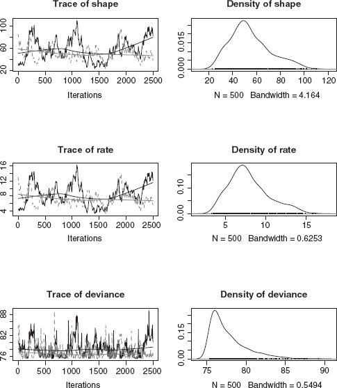
Figure 7.8 WinBUGS output plot: default coda plot, showing trace plots (left) and density plots (right).

7.4 Fitting Challenges

Now that we've reviewed the basic techniques for maximum likelihood and Bayesian estimation, I'll go over some of the special characteristics of problems that make fitting harder.

7.4.1 High Dimensional/Many-Parameter Models

Finding the MLE for a one-parameter model means finding the minimum of the likelihood curve; finding the MLE for a two-parameter model means finding the minimum of a 2D surface; finding the MLE for models with more parameters means finding the minimum on a multidimensional “surface.” Models with more than a few parameters suffer from the curse of dimensionality: the number of parameter combinations, or derivatives, or directions you have to consider increases as a power law of the sampling resolution. For example, if you want find the MLE for a five-parameter model (a pretty simple model) by direct search and you want to subdivide the range of each parameter into 10 intervals (which is quite coarse), you already need 10⁵ parameter combinations. Combine this with function evaluations that take more than a fraction of a second and you're into the better part of a day to do a single optimization run. Direct search is usually just not practical for models with more than two or three parameters.

If you need to visualize a high-dimensional likelihood surface (e.g., examining the region around a putative MLE to see if the algorithm has found a reasonable answer), you'll probably need to look at 2D slices (varying two parameters at a time over reasonable ranges, calculating the objective function for each combination of values while holding all the other parameters constant) or profiles (varying two parameters at a time over reasonable ranges and optimizing over all the other parameters for each combination of values). You are more likely to have to fall back on the information matrix-based approach described in the previous chapter for finding approximate variances and covariances (or correlations) of the parameter estimates; this approach is more approximate and gives you less information than fitting profiles, but extends very simply to any number of parameters.

MCMC fitting adapts well to large models. You can easily get univariate (using HPDinterval from coda for credible intervals or summary for quantiles) and bivariate confidence intervals (using HPDregionplot from emdbook).

7.4.2 Slow Function Evaluations

Since they require many function evaluations, high-dimensional problems also increase the importance of speed in the likelihood calculations. Many of the models you'll deal with take only microseconds to calculate a likelihood, so running tens of thousands of function evaluations can still be relatively quick. However, fitting a high-dimensional model using simulated annealing or other stochastic optimization approaches, or finding confidence limits for such models, can sometimes require millions of evaluations and hours or days to fit. In other cases, you might have to run a complicated population dynamics model for each set of parameters and so each likelihood function evaluation could take minutes or longer (Moorcroft et al., 2006).

Some possible solutions to this problem:

 

•   Use more efficient optimization algorithms, such as derivative-based algorithms instead of Nelder-Mead, if you can.

•   Derive an analytical expression for the derivatives and write a function to compute it. optim and mle2 can use this function (via the gr argument) instead of computing finite differences.

•   Rewrite the code that computes the objective function more efficiently in R. Vectorized operations are almost always faster than for loops. For example, filling a 1000 × 2000 matrix with normally distributed values one at a time takes 30 seconds, whereas picking 2 million values and then reformatting them into a matrix takes only 0.75 second. Calculating the column sums of the matrix by looping over rows and columns takes 20.5 seconds; using apply(m,1,sum) takes 0.13 second; and using colSums(m) takes 0.005 second.

•   If you can program in C or FORTRAN, or have a friend who can, write your objective function in one of these faster, lower-level languages and link it to R (see the R Extensions Manual for details).

•   For really big problems, you may need to use tools beyond R. One such tool is AD Model Builder, which uses automatic differentiation—a very sophisticated algorithm for computing derivatives efficiently—which can speed up computation a lot (R has a very simple form of automatic differentiation built into its deriv function).

•   Compromise by allowing a lower precision for your fits, increasing the reltol parameter in optim. Do you really need to know the parameters within a factor of 10^-8, or would 10^-3 do, especially if you know your confidence limits are likely to be much larger? (Be careful: increasing the tolerance in this way may also allow algorithms to stop prematurely at a flat spot on the way to the true minimum.)

•   Find a faster computer, or break the problem up and run it on several computers at once, or wait longer for the answers.

7.4.3 Discontinuities and Thresholds

Models with sudden changes in the log-likelihood (discontinuities) or derivatives of the log-likelihood, or perfectly flat regions, can cause real trouble for general-purpose optimization algorithms.^* Discontinuities in the log-likelihood or its derivative can make derivative-based extrapolations wildly wrong. Flat or almost-flat regions can make most methods (including Nelder-Mead) falsely conclude that they've reached a minimum.

Flat regions are often the result of threshold models, which in turn can be motivated on simple phenomenological grounds or as the result (e.g.) of some optimal-foraging theories (Chapter 3). Figure 7.9 shows simulated “data” and a likelihood profile/slice for a very simple threshold model. The likelihood profile for the threshold model has discontinuities at the x value of each data point. These breaks occur because the likelihood changes only when the threshold parameter is changed from just below an observed value of x to just above it; adjusting the threshold parameter anywhere in the range between two observed x values has no effect on the likelihood.

The logistic profile, in addition to being smooth rather than choppy, is lower (representing a better fit to the data) for extreme values because the logistic function can become essentially linear for intermediate values, while the threshold function is flat. For optimum values of the threshold parameter, the logistic and threshold models give essentially the same answer. Since the logistic is slightly more flexible (having an additional parameter governing steepness), it gives marginally better fits—but these would not be significantly better according to the Likelihood Ratio test or any other model selection criterion. Both profiles become flat for extreme values (the fit doesn't get any worse for ridiculous values of the threshold parameter), which could cause trouble with an optimization method that is looking for flat regions of the profile.

Figure 7.9 Threshold and logistic models. (a) Data, showing the data (generated from a threshold model) and the best threshold and logistic fits to the data. (b) Likelihood profiles.

Some ways to deal with thresholds:

 

•   If you know a priori where the threshold is, you can fit different models on either side of the threshold.

•   If the threshold occurs for a single parameter, you can compute a log-likelihood profile for that parameter. For example, in Figure 7.9 only the parameter for the location of the threshold causes a problem, while the parameters for the values before and after the threshold are well-behaved. This procedure reduces to direct search for the threshold parameter while still searching automatically for all the other parameters (Barrowman and Myers, 2000). This kind of profiling is also useful when a parameter needs to be restricted to integer values or is otherwise difficult to fit by a continuous optimization routine.

•   You can adjust the model, replacing the sharp threshold by some smoother behavior. Figure 7.9 shows the likelihood profile of a logistic model fitted to the same data. Many fitting procedures for threshold models replace the sharp threshold with a smooth transition that preserves most of the behavior of the model but alleviates fitting difficulties (Bacon and Watts, 1974; Barrowman and Myers, 2000).

7.4.4 Multiple Minima

Even if a function is smooth, it may have multiple minima (e.g., Figure 7.1): alternative sets of parameters that each represent better fits to the data than any nearby parameters. Multiple minima may occur in either smooth or jagged likelihood surfaces.

Multiple minima are a challenging problem, and they are particularly scary because they're not always obvious—especially in high-dimensional problems. Figure 7.10 shows a slice through parameter space connecting two minima that occur in the negative log-likelihood surface of the modified logistic function that Vonesh and Bolker (2005) used to fit data on tadpole predation as a function of size (the function calcslice in the emdbook package will compute such a slice). Such a pattern strongly suggests, although it does not guarantee, that the two points really are local minima. When we wrote the paper, we were aware only of the left-hand minimum, which seemed to fit the data reasonably well. In preparing this chapter, I reanalyzed the data using BFGS instead of Nelder-Mead optimization and discovered the right-hand fit, which is actually slightly better (— L = 11.77 compared to 12.15 for the original fit). Since they use different rules, the Nelder-Mead and BFGS algorithms found their way to different minima despite starting at the same point. This is alarming. While the log-likelihood difference (0.38) is not large enough to reject the first set of parameters, and while the fit corresponding to those parameters still seems more biologically plausible (a gradual increase in predation risk followed by a slightly slower decrease, rather than a very sharp increase and gradual decrease), we had no idea that the second minimum existed. Etienne et al. (2006b) pointed out a similar issue affecting a paper by Latimer et al. (2005) about diversification patterns in the South African fynbos: some estimates of extremely high speciation rates turned out to be spurious minima in the model's likelihood surface (although the basic conclusions of the original paper still held).

Figure 7.10 Likelihood slice connecting two negative log-likelihood minima for the modified logistic model of Vonesh and Bolker (2005). The x axis is on an arbitrary scale where x = 0 and x = 1 represent the locations of the two minima. Subplots show the fits of the curves to the frog predation data for the parameters at each minimum; the right-hand minimum is a slightly better fit (— L = 11.77 (right) vs. 12.15 (left)). The horizontal solid and dashed lines show the minimum negative log-likelihood and the 95% confidence cutoff (—L + x²₁ (0.95)/2). The 95% confidence region includes small regions around both x = 0 and x = 1.

No algorithm can promise to deal with the pathological case of a very narrow, isolated minimum as in Figure 7.1. To guard against multiple-minimum problems, try to fit your model with several different reasonable starting points, and check to make sure that your answers are reasonable.

If your results suggest that you have multiple minima—that is, you get different answers from different starting points or from different optimization algorithms— check the following:

 

•   Did both fits really converge properly? The fits returned by mle2 from the bbmle package will warn you if the optimization did not converge; for optim results you need to check the $convergence term of results (it will be zero if there were no problems). Try restarting the optimizations from both of the points where the optimizations ended up, possibly resetting parscale to the absolute value of the fitted parameters. (If 01 is your first optim fit, run the second fit with control=list(parscale=abs(01$par)). If 01 is an mle2 fit, use control=list(parscale=abs(coef(01))).) Try different optimization methods (BFGS if you used Nelder-Mead, and vice versa). Calculate slices or profiles around the optima to make sure they really look like local minima.

•   Use calcslice to compute a likelihood slice between the two putative fits to make sure that the surface is really higher between them.

 

If your surface contains several minima, the simplest solution may be to use a simple, fast method (like BFGS) but to start it from many different places. This will work if the surface is smooth, but with two (or many) valleys of approximately the same depth.^* You will need to decide how to assign starting values (randomly or on a grid? along some transect?), and how many starting values you can afford to try. You may need to tune the optimization parameters so that each individual optimization runs as fast and smoothly as possible. Researchers have also developed hybrid approaches based on multiple starts (Tucci, 2002).

When multiple minima occur it is possible, although unusual, for the 95% confidence limits to be discontinuous—that is, for there to be separate regions around each minimum that are supported by the data. This does happen in Figure 7.10, although on the scale of that figure the confidence intervals in the regions around x = 0 and x = 1 would be almost too small to see. More frequently, either one minimum will be a lot deeper than the other so that only the region around one minimum is included in the confidence region, or the minima will be about the same height but the two valleys will join at the height of the 95% cutoff so that the 95% confidence interval is continuous.

If the surface is jagged instead of smooth, or if you have a sort of fractal surface— valleys within valleys, of many different depths—a stochastic global method such as simulated annealing is your best bet. Markov chain Monte Carlo can in principle deal with multiple modes, but convergence can be slow—you need to start chains at different modes and allow enough time for each chain to wander to all of the different modes (see Mossel and Vigoda, 2006; Ronquist et al., 2006, for a related example in phylogenetics).

7.4.5 Constraints

The last technical detail covered here is the problem of constraining parameter values within a particular range. Constraints occur for many reasons, but the most common constraints in ecological models are that some parameters make sense only when they have positive values (e.g., predation or growth rates) or values between 0 and 1 (e.g., probabilities). The three important characteristics of constraints concern:

 

1.   Equality vs. inequality: Must a parameter or set of parameters be exactly equal to some value, or just within specified boundaries? Constraints on individual parameters are always inequality constraints (e.g., 0 < p < 1). The most common equality constraint is that probabilities must sum to 1 .

2.   Individual parameters vs. combinations: Are parameters subject to independent constraints, or do they interact? Inequality constraints on individual parameters (a₁ < p₁ < b₁, a₂ < p₂ < b₂) are called box constraints. Constraints on linear combinations of parameters (a₁p₁ + a₂p₂ < c) are called linear constraints.

3.   Solving constraint equations: Can the constraint equations be solved analytically in terms of one of the parameters? For example, you can restate the constraint p₁p₂ = C as p₁ = C/p₂.

In Chapter 8 of the Ecological Detective, Hilborn and Mangel constrain the equilibrium of a complex wildebeest population model to have a particular value. This is the most difficult kind of constraint; it's an equality constraint, a nonlinear function of the parameters, and there's no way to solve the constraint equation analytically.

The simplest approach to inequality constraints is to ignore them completely and hope that your optimizing routine will find a minimum that satisfies the constraint without running into trouble. You can often get away with this if your minimum is far from the boundary, although you may get warning messages that look something like NaNs produced in: dnbinom(x, size, prob, log). If your answers make sense, you can often ignore the warnings, but you should definitely test the results by restarting the optimizer from near its ending point to verify that it still finds the same solution. You may also want to try some of the other constrained approaches listed below to double-check.

The next simplest approach to optimization constraints is to find a canned optimization algorithm that can incorporate constraints in its problem definition. The optim function (and its mle2 wrapper) can accommodate box constraints if you use the L-BFGS-B method. So can nlminb, which was introduced to R more recently and uses a different algorithm. R also provides a constrOptim function that can handle linear constraints. Algorithms that can fit models with general nonlinear equality and inequality constraints do exist, but they have not been implemented in R: they are typically large FORTRAN programs that cost hundreds or thousands of dollars to license (see below for the cheapskate ecologist's approach to nonlinear constraints).

Constrained optimization is finicky, so it's useful to have additional options when one method fails. In my experience, constrained algorithms are less robust than their unconstrained counterparts. For example, L-BFGS-B, the constrained version of BFGS, is (1) more likely to crash than BFGS; (2) worse at handling NAs or infinite values than BFGS; and (3) will sometimes try parameter values that violate the constraints by a little bit when it's calculating finite differences. You can work around the last problem by reducing ndeps and setting boundaries that are a little bit tighter than the theoretical limits, for example, a lower bound of 0.002 instead of 0.

The third approach to constraint problems is to add a penalty to the negative log-likelihood that increases as parameter values stray farther outside the allowed region. Instead of minimizing the negative log-likelihood —L, try minimizing — L + P × | C — C(p)|ⁿ where P is a penalty multiplier, n is a penalty exponent, C is the desired value of the constraint, and C(p) is the value of the constraint at the current parameter values (Hilborn and Mangel, 1997). For example, if you were using P = 1000 and n = 2 (a quadratic penalty, the most common type) and the sum of probabilities for a set of parameters was 1.2 instead of the desired value of 1.0, you would add a penalty term of 1000(1 — 1.2)² = 40 to the negative log-likelihood. The penalty term will tend to push minimizers back into the allowed region. However, you need to implement such penalties carefully. For example, if your likelihood calculation is nonsensical outside the allowed region (e.g., if some parameters lead to negative probabilities), you may need to use the value of the negative log-likelihood at the closest boundary rather than trying to compute — L for parameters outside the boundary. If your penalties make the surface nonsmooth at the boundary, derivative-based minimizers are likely to fail. You will often need to tune the penalty multiplier and exponent, especially for equality constraints.

The fourth, often most robust, approach is to transform your parameters to avoid the constraints entirely. For example, if you have a rate or density parameter λ that must be positive, rewrite your function and minimize with respect to x = log λ instead. Every value of x between —∞ and ∞ translates to a positive value of λ negative values of x correspond to values of λ < 1. As x approaches —∞, λ approaches zero; as x approaches λ ∞ also approaches ∞.

Similarly, if you have a parameter p that must be between 0 and 1 (such as a parameter representing a probability), the logit transformation of p, q = log (p/ (1 — p)), will be unconstrained (its value can be anywhere between —∞ and ∞). You can use qlogis in R to calculate the logit. The inverse transformation is the logistic transformation, exp (q)/(1 + exp (q)) (plogis).

The log and logit transformations are by far the most common transformations. Many classical statistical methods use them to ensure that parameters are well defined; for example, logistic regression fits probabilities on a logit scale. Another less common but still useful transformation is the additive log ratio transformation (Aitchison, 1986; Billheimer et al., 1998; Okuyama and Bolker, 2005). When you're modeling proportions, you often have a set of parameters p₁,…, p_n representing the probabilities or proportions of a variety of outcomes (e.g., predation by different predator types). Each p_i must be between 0 and 1, and . The sum-to-one constraint means that the constraints are not box constraints (which would apply to each parameter separately), and even though it is linear, it is an equality constraint rather than a inequality constraint—so constrOptim can't handle it. The additive log ratio transformation takes care of the problem: the vector is a set of n — 1 unconstrained values from which the original values of pi can be computed. There is one fewer additive log-ratio-transformed parameter because if we know n — 1 of the values, then the nth is determined by the summation constraint. The inverse transformation (the additive logistic) is .

The major problem with transforming constraints this way is that sometimes the best estimates of the parameters, or the null values you want to test against, actually lie on the boundary—in mixture or composition problems, for example, the best fit may set the contribution from some components equal to zero. For example, the best estimate of the contribution of some turtle nesting beaches (rookeries) to a mixed foraging-ground population may be exactly zero (Okuyama and Bolker, 2005). If you logit-transform the proportional contributions from different nesting beaches, you will move the lower boundary from 0 to —∞. Any optimizer that tries to reach the boundary will have a hard time, resulting in warnings about convergence and/or large negative estimates that differ depending on starting conditions. One option is simply to set the relevant parameters to zero (i.e., construct a reduced model that eliminates all nesting beaches that seem to have minimal contributions), estimate the minimum negative log-likelihood, and compare it to the best fit that the optimizer could achieve. If the negative log-likelihood is smaller with the contributions set to zero (e.g., the negative log-likelihood for contribution = 0 is 12.5, compared to a best-achieved value of 12.7 when the log-transformed contribution is —20), then you can conclude that zero is really the best fit. You can also compute a profile (negative log-)likelihood on one particular contribution with values ranging upward from zero and see that the minimum really is at zero. However, going to all this trouble every time you have a parameter or set of parameters that appear to have their best fit on the boundary is quite tedious.

One final issue with parameters on the boundary is that the standard model selection machinery discussed in Chapter 6 (Likelihood Ratio Test, AIC, etc.) always assumes that the null (or nested) values of parameters do not lie on the boundary of their feasible range. This issue is well-known but still problematic in a wide range of statistical applications, for example, in deciding whether to set a variance parameter to zero. For the specific case of linear mixed-effect models (i.e., models with linear responses and normally distributed random variables), the problem is relatively well studied. Pinheiro and Bates (2000) suggest the following approaches (listed in order of increasing sophistication):

 

•   Simply ignore the problem, and treat the parameter as though it were not on the boundary—i.e., use a likelihood ratio test with 1 degree of freedom. Analyses of linear mixed-effect models (Self and Liang, 1987; Stram and Lee, 1994) suggest that this procedure is conservative; it will reject the null hypothesis less often (sometimes much less often) than the nominal type I error rate α.^*

•   Some analyses of mixed-effect models suggest that the distribution of the log-likelihood ratio under the null hypothesis when n parameters are on the boundary is a mixture of and distributions rather than a distribution. If you are testing a single parameter, as is most often the case, then n = 1 and is —defined as a spike at zero with area 1. For most models, the distribution is a 50/50 mixture of and , which Goldman and Whelan (2000) call the distribution. For In this case the 95% critical value for the likelihood ratio test would thus be (0.95)/2 = qchisq(0.9,1)/2=1.35 instead of the usual value of 1.92. The qchibarsq function in the emdbook package will compute critical values for .

•   The distribution of deviances may not be an equal mixture of and (Pinheiro and Bates, 2000). The “gold standard” is to simulate the null hypothesis and determine the distribution of the log-likelihood ratio under the null hypothesis; see Section 7.6.1 for a worked example.

7.5 Estimating Confidence Limits of Functions of Parameters

Quite often, you estimate a set of parameters from data, but you actually want to say something about a value that is not a parameter (e.g., about the predicted population size some time in the future). It's easy to get the point estimate—you just feed the parameter estimates into the population model and see what comes out. But how do you estimate the confidence limits on that prediction?

There are many possibilities, ranging in accuracy, sophistication, and difficulty. The data for an extended example come from J. Wilson's observations of “death” (actually disappearance, which may also represent emigration) times of juvenile reef gobies in a variety of experimental treatments. The gobies' times of death are assumed to follow a Weibull distribution:

The Weibull distribution (dweibull in R), common in survival analysis, allows for a per capita mortality rate that either increases or decreases with time. It is shaped like the Gamma distribution, ranging from L-shaped to humped (normal). It has two parameters, shape (a above) and scale (b above): when shape = 1 it reduces to an exponential. It's straightforward to calculate the univariate or bivariate confidence limits of these parameters, but what if we want to calculate the confidence interval of the mean survival time, which is likely to be more meaningful to the average ecologist or manager?

First, pull in the data and take a useful subset:

Define the death time as the midpoint between the last time the fish was observed (d1) and the first time it was not observed (d2):^†

Set up a simple likelihood function:

Fit the model starting from an exponential distribution (if shape = a = 1, the distribution is an exponential with rate 1/b and mean b):

Figure 7.11 Geometry of confidence intervals on mean survival time. Gray contours: univariate (80%, 90%, 95%, 99%) confidence intervals for shape and scale. Black contours: mean survival time. Dotted line: likelihood profile for mean survival time.

The parameter estimates (coef(w1)) are shape = 0.921 and scale = 14.378; the estimate of the mean survival time (using the information on p. 253) is 14.945 days.

7.5.1 Profile Likelihood

Now we'd like confidence intervals for the mean that take variability in both shape and scale into account. The most rigorous way to estimate confidence limits on a nonparameter is to calculate the profile likelihood for the value and find the 95% confidence limits, using almost the same procedure as if you were finding the univariate confidence limits of one of the parameters.

Figure 7.11 illustrates the basic geometry of this problem: the underlying contours of the height of the surface (contours at 80%, 90%, 95%, and 99% univariate confidence levels) are shown in gray. The black contours show the lines on the plot that correspond to different constant values of the mean survival time. The dotted line is the likelihood profile for the mean, which passes through the minimum negative log-likelihood point on each mean contour, the point where the mean contour is tangent to a likelihood contour line. We want to find the intersections of the Likelihood Ratio Test contour lines with the likelihood profile for the mean; looking at the 95% line, we can see that the confidence intervals of the mean are approximately 9 to 27.

7.5.1.1

THE VALUE CAN BE EXPRESSED IN TERMS OF OTHER PARAMETERS

When the value for which you want to estimate confidence limits has a formula that you can solve in terms of one of the parameters, calculating its confidence limits is easy.

For the Weibull distribution the mean μ is given by

or, translating to R,

How do we actually calculate the profile for the mean? We can solve (7.5.2) for one of the parameters:

Therefore, we can find the likelihood profile for the mean in almost the same way we would for one of the parameters. Fix the value of μ then, for each value of the shape that R tries on its way to estimating the parameter, it will calculate the value of the scale that must apply if the mean is to be fixed at μ. The constraint means that, even though the model has two parameters (shape and scale), we are really doing a one-dimensional search, which just happens to be a search along a specified constant-mean contour.

To calculate the confidence interval on the mean, we have to rewrite the likelihood function in terms of the mean:

Find the maximum again, and calculate the confidence intervals—this time for the shape and the mean.

We could also draw the univariate likelihood profile, the minimum negative log-likelihood achievable for each value of the mean, and find the 95% confidence limits in the same way as before by creating a likelihood profile for μ. We would use 1 degree of freedom to establish the critical value for the LRT because we are varying only one value, even though it represents a combination of two parameters.

7.5.1.2 CONSTRAINED/PENALIZED LIKELIHOOD

What if we can't solve for one of the parameters (e.g., scale) in terms of the value we are interested in (e.g., mean), but still want to calculate a likelihood profile and profile confidence limits for the mean? We can use a penalized likelihood function to constrain the mean to a particular value, as described above in the section on constraints.

While this approach is conceptually the same as the one we took in the previous section—we are calculating the profile by sliding along each mean contour to find the minimum negative log-likelihood on that contour, then finding the values of the mean for which the minimum negative log-likelihood equals the LRT cutoff—the problem is much fussier numerically. (The complicated code is presented on p. 259.) To use penalties effectively we usually have to play around with the strength of the penalty. Too strong, and our optimizations will get stuck somewhere far away from the real minimum. Too weak, and our optimizations will wander off the line we are trying to constrain them to. I tried a variety of penalty coefficients P in this case (penalty = P × (deviation of mean survival from target value)²) from 0.1 to 10⁶. The results were essentially identical for penalties ranging from 1 to 10⁴ but varied for weaker or stronger penalties. One might be able to tweak the optimization settings some more to make the answers better, but there's no simple recipe—you just have to keep returning to the pictures to see if your answers make sense.

7.5.2 The Delta Method

The delta method provides an easy approximation for the confidence limits on values that are not parameters of the model. To use it you must have a formula for μ = f (a, b) that you can differentiate with respect to a and b. Unlike the first likelihood profile method, you don't have to be able to solve the equation for one of the parameters.

The formula for the delta method comes from a Taylor expansion of the formula for μ, combined with the definitions of the variance and covariance :

See the appendix or Lyons (1991) for details.

We can obtain approximate variances and covariances of the parameters by taking the inverse of the information matrix: vcov does this automatically for mle2

We also need the derivatives of the function with respect to the parameters. In this example these are the derivatives of with respect to shape = a and scale = b. The derivative with respect to b is easy——but is harder. By the chain rule

but in order to finish this calculation you need to know that d(x)/dx = (x). digamma(x), where digamma is a special function (defined as the derivative of the log-gamma function). The good news is that R knows how to compute this function, so

will give you the right numeric answer. The emdbook package has a built-in deltavar function that uses the delta method to compute the variance of a function:

Once you find the variance of the mean survival time, you can take the square root to get the standard deviation π and calculate the approximate confidence limits μ ± 2π (use meanfun, defined on p. 253, to compute the value of μ).

If you can't compute the derivatives analytically, R's numericDeriv function will compute them numerically (p. 261).

7.5.3 Population Prediction Intervals (PPIs)

Another simple procedure for calculating confidence limits is to draw random samples from the estimated sampling distribution (approximated by the information matrix) of the parameters. In the approximate limit where the information matrix approach is valid, the distribution of the parameters will be multivariate normal with a variance-covariance matrix given by the inverse of the information matrix. The MASS package in R has a function, mvrnorm,^*for selecting multivariate normal random deviates. With the mle2 fit w1 from above,

will select 1000 sets of parameters drawn from the appropriate distribution (if there are n parameters, the answer is a 1000 × n matrix). (If you have used optim instead of mle2 —suppose opt1 is your result—then use opt1$par for the mean and solve(opt1$hessian) for the variance.) You can then use this matrix to calculate the estimated value of the mean for each of the sets of parameters, treat this distribution as a distribution of means, and find its lower and upper 95% quantiles (Figure 7.12). In the context of population viability analysis, Lande et al. (2003) refer to confidence intervals computed this way as “population prediction intervals.”

This procedure is easy to implement in R, as follows:

Figure 7.12 Population prediction distribution and Bayesian posterior distribution of mean survival time, with confidence and credible intervals.

Calculating population prediction intervals in this way has two disadvantages:

 

•   It blurs the line between frequentist and Bayesian approaches. Many papers (including some of mine, e.g., Vonesh and Bolker (2005)) have used this approach, but I have yet to see a solidly grounded justification for propagating the sampling distributions of the parameters in this way.

•   Since it uses the asymptotic estimate of the parameter variance-covariance matrix, it inherits whatever inaccuracies that approximation introduces. It makes one fewer assumption than the delta method (it doesn't assume the variance is so small that the functions are close to linear), but it may not be much more accurate.

7.5.4 Bayesian analysis

Finally, you can use a real Bayesian method: construct either an exact Bayesian model or, more likely, a Markov chain Monte Carlo analysis for the parameters. Then you can calculate the posterior distribution of any function of the parameters (such as the mean survival time) from the posterior samples of the parameters, and get the 95% credible interval.

The hardest part of this analysis is converting between R and WinBUGS versions of the Weibull distribution: where R uses , WinBUGS uses . Matching up terms and doing some algebra shows that v = a and λ = b^–a or b = λ^–1/a.

The BUGS model is

Other differences between R and WinBUGS are that BUGS uses pow(x,y) instead of xˆy and has only a log-gamma function loggam instead of R's gamma and lgamma functions. The model includes code to convert from WinBUGS to R parameters (i.e., calculating scale as a function of lambda) and to calculate the mean survival time, but you could also calculate these values in R.

Set up three chains that start from different, overdispersed values of shape and λ:

Run the chains assuming that the model is stored in a file called reefgobysurv.bug:

Finally, use HPDinterval or summary to extract credible intervals or quantiles from the MCMC output. Figure 7.12 compares the marginal posterior density of the mean and the credible intervals computed from it with the distribution of the mean derived from the sampling distribution of the parameters and the population prediction intervals (Section 7.5.3).

TABLE 7.2
Confidence intervals on mean survival for goby data

7.5.5 Confidence Interval Comparison

Table 7.2 presents a head-to-head comparison of all the methods we've applied so far. All methods give approximately the same answers. Despite answering a different question, the Bayes credible interval is in the same range as the other confidence intervals. The point to take away from this comparison is that all methods for estimating confidence limits use approximations, some cruder than others. Use the most accurate feasible approach, but don't expect estimates of confidence limits to be very precise. To paraphrase a comment of Press et al. (1994), if the difference between confidence-interval approximations ever matters to you, “then you are probably up to no good anyway—e.g., trying to substantiate a questionable hypothesis with marginal data.”^*

7.6 R Supplement

7.6.1

Testing Hypotheses on Boundaries by Simulating the Null Hypothesis

Suppose you want to test the hypothesis that the data set

comes from a negative binomial distribution against the null hypothesis that it is Poisson distributed with λ = = 1.35.

A negative binomial fit (fit.nb=fitdistr(x,”negative binomial”)) gives a negative log-likelihood (-logLik(fit.nb)) of 31.38, while a Poisson fit (fit.pois=fitdistr(x,”Poisson”)) gives a negative log-likelihood of 32.12. The Likelihood Ratio test

says that the p-value is 0.22, but the corrected (x^-2₁) test (pchibarsq(devdiff,df=1, lower.tail=FALSE)) says that p is only 0.12—still not significant at p = 0.05 but stronger evidence.

To evaluate the hypothesis more thoroughly by simulation, we will set up a function with no arguments that (1) simulates Poisson-distributed values with the appropriate mean; (2) fits a negative binomial and Poisson distributions (returning NA if the negative binomial fit should happen to crash); and (3) returns the deviance (twice the log-likelihood ratio):

Now simulate 3000 such values, throw out the NAs, and count the number of replicates remaining:

Calculate the proportion of simulated values that exceed the observed deviance: this is the best estimate of the “true” p-value we can get.

So, in this case where we have two reasons—small sample size and a boundary condition—to doubt the assumptions of Likelihood Ratio Test, the classical LRT turns out to be nearly four times too conservative, while the boundary-corrected version (x^-2) is only twice as conservative as it should be.

7.6.2 Nonlinear Constraints by Penalization

Using penalties to implement an equality constraint or a nonlinear constraint (neither of which can be done with built-in functions in R) is reasonably straightforward: just add a penalty term to the negative log-likelihood. For best results, the penalty should start small and increase with increasing violation of the constraint, to avoid a discontinuity in the negative log-likelihood surface.

For example, to find the best shape and scale parameters for the fish survival data while constraining the mean to equal a particular value target.mu (use the fixed argument in mle2 to specify the target value):

If you have a problem where the function behaves badly (generates infinite or NaN values) when the constraint is violated, then you don't want to calculate the likelihood for values outside the constraints. For example, if we had to restrict shape to be greater than zero, we could use the following code snippet:

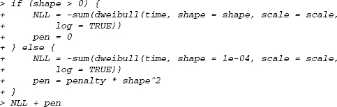
In other words, if the shape parameter is beyond the constraints, then use the likelihood value at or near the boundary of the feasible region and then add the penalty.

To use this constrained likelihood function to calculate confidence limits on the mean, first calculate the critical value of the negative log-likelihood:

Second, define a function that finds the best fit for a specified value of the mean and returns the distance above the critical value (use the data argument in mle2 so that you can try out different values of the penalty):

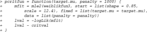
Third, define the range of mean values in which you think the lower confidence limit lies and use uniroot to search within this range for the point where the negative log-likelihood is exactly equal to the critical value:

Do the same for the upper confidence limit:

Try with a different value of the penalty:

7.6.3 Numeric Derivatives

Analytical derivatives are always faster and more numerically stable, but R can compute numeric derivatives for you. For example, to compute the derivatives of the mean survival time at the maximum likelihood estimate:

(The quote inside the numericDeriv command prevents R from evaluating the expression prematurely.) Of course, you can always do the same thing yourself by hand:

7.6.4

Extracting Information from BUGS and CODA Output

R2WinBUGS returns its results as a bugs object, which can be plotted or printed. The as.mcmc function in the emdbook package will turn this object into an mcmc.list object for a multichain run or an mcmc object for a single-chain run. read.bugs in the R2WinBUGS package does the same thing, but it requires an extra step. The mcmc and mcmc.list objects are more flexible—they can be plotted and summarized in a variety of ways (summary, HPDinterval, densityplot…; see the help for the coda package). Once you ensure that the chains in a multichain R2WinBUGS run have converged, you can use lump.mcmc.list in the emdbook package to collapse the mcmc.list object so you can draw inferences from the combined chains.

Using the reefgoby.bugs object derived from the WinBUGS run on p. 257, calculate the Bayesian credible interval:

Appendix: Trouble-Shooting Optimization

•   Make sure you understand the model you're fitting.

•   Check starting conditions.

•   Check convergence conditions.

•   Adjust parscale/restart from previous best fit.

•   Switch from constraints to transformed parameters.

•   Adjust finite-difference tolerances (ndeps).

•   Switch to more robust methods (Nelder-Mead, SANN), or even just alternate methods.

•   Optimization stops with NAs: debug objective function, constrain parameters, put if clauses in objective function.

•   Results depend on starting conditions: check slices between and around answers: multiple minima or just convergence problems?

•   Convergence problems: try restarting from previous stopping point, resetting parscale.

•   Examine profile likelihoods.

 

 

---

^* mle and mle2 use method=“BFGS” by default. Nelder-Mead optimization (see below) is unreliable in one dimension and R will warn you if you try to use it to optimize a single parameter.

^† The Nelder-Mead simplex is completely unrelated to the simplex method in linear programming, which is a method for solving high-dimensional linear optimization problems with constraints.

^‡ However, you need to specify only a single starting point; R automatically creates a simplex around your starting value.

^* The chain must be irreducible (it must be possible eventually to move from any point in parameter space to any other) and aperiodic (it should be impossible for it to get stuck in a loop).

^‡ In the simulated annealing rule we exponentiated — k times the log-likelihood difference, which gave us the likelihood ratio raised to the power —k; if we set k = 1, then we have L_old/L_new, which corresponds to Post(A)/Post(B).

^* They specifically suggested:

1. Set the tuning parameter much larger than normal so that the acceptance rate is actually below the usual 20-25% rule of thumb. This will fatten and lengthen the proposal distribution so that one can jump from one tail to the other.

2. Forgo the proposal distribution based on the large sample var-cov matrix. Set the V parameter in MCMCmetrop1R to something that will work reasonably well over the entire parameter space.

3. Use an MCMC algorithm other than the random walk Metropolis algorithm. You'll need to use something other than MCMCmetrop1R to do this, but this option will be the most computationally efficient.

^* I will focus on a text file description, and on the R interface to WinBUGS implemented in the R2WinBUGS package, but many different variants of automatic Gibbs samplers are springing up. These vary in interface, degree of polish, and supported platforms. (1) WinBUGS runs on Windows and under WINE on Linux and Intel Macs; models can be defined either graphically or as text files; R2WinBUGS is the R interface. (2) OpenBUGS (http://mathstat.helsinki.fi/openbugs/) is a new version of WinBUGS that runs on the same platforms as WinBUGS and has an R interface, BRugs. (3) JAGS is an alternative automatic sampler that runs on Linux, Windows, and MacOS and has an R interface, rjags.

^* In a few years this list of citations will probably be too long to include!

^* Specialized algorithms, such as those included in the segmented package on CRAN, can handle certain classes of piecewise models (Muggeo, 2003).

^* The many-valley case, or rather its inverse the many-peaks case (if we are maximizing rather than minimizing), is sometimes known as a “fakir's bed” problem after the practice of sitting on a board full of nails (Swartz, 2003).

^* The emdbookx package contains data that have not yet been generally released; please contact me for access.

^‡ Survival analyses usually assume that the time of death is known exactly. With these data, as is common in ecological studies, we have a range of days during which the fish disappeared. To handle this so-called interval censoring properly in the likelihood function, we would have to find the probability of dying after day d1 but before day d2, which is (probability of dying before d2 — probability of dying before d1). In R the negative log-likelihood function would be

For this example, I’ve used the cruder, simpler approach of averaging d1 and d2.

^* mvrnorm should really be called rmvnorm for consistency with R's other distribution functions, but S-PLUS already has a built-in function called rmvnorm, so the MASS package had to use a different name.

^* Their original statement referred to whether to divide by n or n — 1 when estimating a variance.