The word “logic” has many meanings, and is heavily overloaded. It’s derived from the Greek word logicos, meaning “concerning language and speech” or “human reasoning.”

The section “The History of Logic” gives a concise overview of the history of logic, just to show that many brilliant people have been involved over several centuries to develop what’s now known as mathematical logic. The section is by no means meant to be complete.

In the section “Values, Variables, and Types,” we’ll discuss the difference between values (constants) and variables. We’ll also introduce the notion of the type of a variable. We’ll use these notions in the section “Propositions and Predicates” to introduce the concept of a predicate, and its special case, a proposition—the main concepts in logic.

The section “Logical Connectives” explains how you can build new predicates by combining existing predicates using logical connectives. Then, in the section “Truth Tables” you’ll see how you can use truth tables to define logical connectives and to investigate the truth value of logical expressions. Truth tables are an important and useful tool to start developing various concepts in logic.

Functional completeness is covered in the section “Functional Completeness”; it’s about which logical connectives you need (as a minimum) to formulate all possible logical expressions.

The following two sections introduce the concepts of tautologies and contradictions, logical equivalence, and rewrite rules. You can use a rewrite rule to transform one logical expression into another (equivalent) logical expression.

This chapter is an introductory chapter onc logic. Chapter 3 will continue where this one stops—the two chapters make up one single topic (logic). The split is necessary because some concepts concerning logic require the introduction of a few set-theory notions first. Chapter 2 will serve that purpose.

The introduction of the crucial concept of rewrite rules at the end of this chapter opens up the first possibility to do some useful exercises. They serve two important purposes:

• Learning how to use truth tables and rewrite rules to investigate logical expressions
• Getting used to the mathematical symbols introduced in this chapter

Therefore, we strongly advise you to spend sufficient time on these exercises before moving on to other chapters.

The History of Logic

The science of logic and the investigation of human reasoning goes back to the ancient Greeks, more than 2,000 years ago. Aristotle (384–322 BC), a student of Plato, is commonly considered the first logician.

Gottfried Wilhelm Leibnitz (1646–1716) established the foundations for the development of mathematical logic. He thought that symbols were extremely important to understand things, so he tried to design a universal symbolic language to describe human reasoning. The logic of Leibnitz was based on the following two principles:

• There are only a few simple ideas that form the “alphabet of human thought.”
• You can generate complex ideas from those simple ideas by a process analogous to arithmetical multiplication.

George Boole (1815–1864) invented the general concept of a Boolean algebra, the foundation of modern computer arithmetic. In 1854 he published An Investigation of the Laws of Thought on Which Are Founded the Mathematical Theories of Logic and Probabilities, in which he shows that you can perform arithmetic on logical symbols just like algebraic symbols and numbers.

In 1922, Ludwig Wittgenstein (1889–1951) introduced truth tables as we know them today, based on the earlier work of Gottlob Frege (1848–1925) and others during the 1880s.

After a formal notation was introduced, several attempts were made to use mathematical logic to describe the foundation of mathematics itself. The attempt by Gottlob Frege (that failed) is famous; Bertrand Russell (1872–1970) showed in 1901 that Frege’s system could produce a contradiction: the famous Russell’s paradox (see sidebar). Later attempts to achieve the same goal were performed by Bertrand Russell and Alfred North Whitehead (1861–1947), David Hilbert (1862–1943), John von Neumann (1903–1957), Kurt Gödel (1906–1978), and Alfred Tarski (1902–1983), just to name a few of the most famous ones.

RUSSELL’S PARADOX

It’s safe to say that the science of logic is sound; it has existed for many centuries and has been investigated by many brilliant scientists over those centuries.

These days, formal methods derived from logic are not only used in mathematics, informatics (computer science), and artificial intelligence; they are also used in biology, linguistics, and even in jurisprudence.

The importance of data management being based on logic was envisioned by E. F. (Ted) Codd (1923–2003) in 1969, when he first proposed his famous relational model in the IBM research report “Derivability, Redundancy and Consistency of Relations Stored in Large Data Banks.” The relational model for database management introduced in this research report has proven to be an influential general theory of data management and remains his most memorable achievement.

Every science is (should be) based on logic: every theory is a system of sentences (or statements) that are accepted as true and can be used to derive new statements following some well-defined rules. It’s one of the main goals of this book to explain the mathematical concepts on which the science of relational data management is based.

Values, Variables, and Types

You probably have some idea of the two terms values and variables. However, it’s important to define these two terms precisely, because they are often misunderstood and mixed up.

A value is an individual constant with a well-determined meaning. For example, the integer 42 is a value. You cannot update a value; if you could, it would no longer be the same value. Values can be represented in many ways, using some encoding. Values can have any arbitrary complexity.

A variable is a holder for a value. Variables in the course of time and space get a different value. We call the changing of values the updating of a variable. Variables have a name, allowing you to talk about them without knowing which value they currently represent.

In this book, we’ll always use variables that are of a given type. The set of values from which the variable is allowed to hold a value is referred to as the type of that variable.

A database—containing table values—is an example of a variable; at any point in time, it has a certain (complex) value. We will specify the type of a database variable in a precise way in Part 2 of this book.

Propositions and Predicates

In logic, the main components we deal with are propositions and predicates. A proposition is a declarative sentence that’s either TRUE or FALSE.

If a proposition is true we say it has a “truth value” of TRUE; if a proposition is false, its truth value is FALSE. Here are some examples of propositions:

• This book has two authors.
• The square root of 16 equals 3.
• All mathematicians are liars.
• If Toon is familiar with SQL, then Lex has three daughters.

All four examples are declarative sentences; if you prefix them with “Is it true that,” then a proper English question is formed and you can decide if the declarative sentences are TRUE or not. The truth value of the first proposition is TRUE; it is a TRUE proposition. The second proposition is obviously FALSE; the square root of 16 equals 4. The third example is a proposition too, although you might find it difficult to decide what its truth value is. But in theory you can decide its truth value. Assuming you have a clear definition of who is and who isn’t a mathematician, you can determine the set of persons that need to be checked. You would then have to check every mathematician, in this rather large but finite set, to find the truth value of the proposition. If you find a non-lying mathematician, then the proposition is FALSE; on the other hand, if no such mathematician can be found, then the proposition is clearly TRUE. In the last example, “Toon” and “Lex” are the authors of this book. Therefore, you should be able to decide whether this predicate is TRUE or FALSE if you know enough about the authors of this book. The proposition is FALSE, by the way; Toon is indeed familiar with SQL, but Lex does not have three daughters.

The following examples are not propositions:

• x + y > 10
• The square root of x equals z.
• What did you pay for this book?
• Stop designing databases.

The first two examples hold embedded variables; the truth value of these sentences depends on the values that are currently held by these variables. The last two examples aren’t declarative sentences and therefore aren’t propositions.

A predicate is something having the form of a declarative sentence. A predicate holds embedded variables whose values are unknown at this time; you cannot decide if what is declared is either TRUE or FALSE without knowing the value(s) for the variable(s). We’ll refer to the embedded variables in a predicate as the parameters of the predicate.

The first two examples in the preceding list are predicates; they hold embedded variables x, y, and z. Following are some other examples of predicates:

• i has the value 4.
• x lives in y.
• If Toon is familiar with SQL, then Lex has k daughters.

You cannot tell if the first example is TRUE or FALSE, because it depends on the actual value of parameter i. The same holds for the second example; as long as you don’t know which human being is represented by parameter x and which city is represented by parameter y, you cannot say whether this predicate is TRUE or FALSE. Finally, the truth value of the last example depends on its parameter k. You already saw that if value 3 is substituted for parameter k, then the truth value of this predicate becomes FALSE.

A predicate with n parameters is called an n-place predicate. If you substitute one of the parameters in an n-place predicate with a value, then the predicate becomes an (n-1)-place predicate. For instance, the preceding second example is a 2-place predicate; it has two parameters, x and y. If you substitute the value Lex for parameter x, then this predicate turns into the following expression:

This expression represents a 1-place predicate; it has one parameter. The truth value still depends upon (the value of) the remaining parameter. If you now substitute value “Utrecht”—the name of a city in the Netherlands—for parameter y, the predicate turns into a 0-place predicate.

Do you see that this is now a proposition? You can decide the truth value of this expression. As this example shows, propositions can be regarded as a special case of predicates; they are predicates with no parameters. You can convert a predicate into a proposition by providing values that are substituted for the parameters. This is called instantiating the predicate with the given values.

The parameters of a predicate are also referred to as the free variables of a predicate. There’s another way to convert predicates into propositions: by binding the involved free variable(s) with a quantifier. Free variables then turn into what are called bound variables. Quantification (over a set) is an important concept in logic and even more so in data management; we’ll cover it in Chapter 3 (the section “Quantifiers”) in great detail.

Table 1-1 summarizes the properties of a predicate and a proposition.

Table 1-1. Predicates and Propositions

Predicate	Proposition
Form of declarative sentence	Declarative sentence
With parameters	Without parameters
Truth-valued function	Either TRUE or FALSE
Input is required to evaluate truth/falsehood	Special case predicate (no input required)

Before we go on, let’s briefly look at sentences such as the following:

These are self-referential sentences; they say something about themselves. Sentences of this type can cause trouble in the sense that they might lead to a contradiction. The second example is known as the liar’s paradox. If you assume these sentences to be TRUE then you can draw the conclusion that they are FALSE (and vice versa); you cannot decide whether they are TRUE or FALSE, which is a mandatory property for them to be valid propositions. The solution is simply to disqualify them as valid propositions.

You must also discard “ill-formed” expressions as valid predicates; that is, expressions that don’t adhere to our syntax rules, such as the following:

The first one is ill-formed because 4 is not a set; it is a numeric value. To say 3 is an element of it doesn’t make any sense. Here we assume you have some idea of the concept of a set and for something to be an element of a set; we’ll cover elementary set theory in Chapter 2. The second expression contains two consecutive connectives ∨ and ∧ (explained in the next section), which is illegal.

Logical Connectives

You can build new predicates by applying logical connectives to existing ones. The most well-known connectives are conjunction (logical AND), disjunction (logical OR), and negation (logical NOT); two other connectives we’ll use frequently are implication and equivalence. Throughout this book, we use mathematical symbols to denote these logical connectives, as shown in Table 1-2.

We’ll precisely define the meaning of these five logical connectives in the section “Truth Tables” when the concept of a truth table is introduced.

Simple and Compound Predicates

Logical connectives can be regarded as logical operators; they take one or more predicates as their operands, and return another predicate. For instance, the logical AND in Table 1-2 has n = 4 and m = 2 as its operands (inputs) and returns the predicate listed under the Example column as its output predicate. We say that the AND operator is invoked with operands n = 4 and m = 2.

It’s quite common to refer to predicates without logical connectives as simple predicates, and to refer to predicates with one or more logical connectives as compound predicates. The input predicates (operands) of a connective in a compound predicate are also referred to as the components of that predicate.

Another common term is the complexity of a compound predicate, which is the number of connectives occurring in that predicate. Here are some more examples of compound predicates, this time using the mathematical symbols.

• n = 4 ∧ m = 5
• x = 42 ∨ x ≠ 42
• Toon lives in Utrecht ⇒ 1 + 1 = 2
• P ∧ Q ⇒ P ⇒ Q

In the last example, P and Q are propositional variables. They denote an arbitrary proposition with an unspecified truth value. We’ll use letters P, Q, R, and so on for propositional variables. You can use propositions, as well as propositional variables, to form new assertions using the logical connectives introduced in the preceding text. An assertion that contains at least one propositional variable is called a propositional form. If you substitute propositions for the variables of a propositional form, a proposition results.

In a similar way, we’ll use the letters P, Q, R, and so on in expressions such as P(x), Q(s,t), R(y), and so on to denote arbitrary predicates with at least one parameter. The parameter(s) of such predicates are denoted by the letters—in these cases x, y, s, and t—separated by commas inside the parentheses of these expressions. For instance, the first compound predicate listed in the preceding text can be denoted as P(n,m). If we substitute the value 3 for the parameter n and the value 5 for the parameter m, the predicate changes to a proposition P(3,5) whose truth value is FALSE.

In mathematics, the precise meaning (semantics) of all logical connectives can be defined using truth tables, as introduced in the next section. With those definitions, you can “calculate” the truth values of compound predicates from the truth values of their components.

Using Parentheses and Operator Precedence Rules

You can use parentheses in logical expressions to denote operator precedence, just like in regular arithmetic, where you can overrule the customary operator precedence as defined by the mnemonic “Please Excuse My Dear Aunt Sally.”

Even when a language defines formal operator precedence rules—allowing you to omit parentheses in certain expressions—it still is a good idea to use them for enhanced readability. It isn’t wrong to include parentheses that could be omitted without changing the meaning. You can include parentheses into the previous four compound predicate examples as follows:

• ( n = 4 ) ∧ ( m = 5 )
• ( x = 42 ) ∨ ( x ≠ 42 )
• ( Toon lives in Utrecht ) ⇒ ( 1 + 1 = 2 )
• ( P ∧ Q ) ⇒ ( P ⇒ Q )

The readability of the last example is definitely enhanced by including the parentheses. It’s customary to adopt the precedence rules as shown in Table 1-3 for the five logical connectives we introduced so far (note that some have the same rank).

Table 1-3. Logical Connective Precedence Rules

Rank	Connective
1	¬
2	∧, ∨
3	⇒, ⇔

These precedence rules prescribe that, for example, the following compound predicate P ∧ Q ⇒ R—which has no included parentheses—should in fact be interpreted as (P ∧ Q) ⇒ R—not as P ∧ (Q ⇒ R), which is a different predicate (that is, it has a different meaning). When same-rank connectives are involved, it’s customary to have them associate their operands from right to left; this is sometimes referred to as the associativity rule. This means that the predicate P ⇒ Q ⇒ R should in fact be interpreted as P ⇒ (Q ⇒ R).

Consider the following two example predicates, and check out the usage of parentheses:

1. ¬ ( P ⇒ Q ) ⇔ ( P ∧ ¬Q )
2. ( ( P ⇒ Q ) ∧ ( Q ⇒ R ) ) ⇒ ( P ⇒ R )

In the first example, the first set of parentheses is needed—otherwise the negation would affect P only. The second set can be omitted, because ∧ takes precedence over ⇔. In the second example, the outermost parentheses at the left-hand side are optional, as are the parentheses at the right-hand side (due to the associativity rule), but the other two sets of parentheses are needed.

In the remainder of this book when more than one connective is involved in a predicate, we’ll always include parentheses and not depend on the precedence and associativity rules.

Truth Tables

Truth tables are primarily used in logic to establish the basic logical concepts. You can use them for two (quite different) basic purposes:

• To define the meaning of logical connectives
• To investigate the truth value of compound logical expressions

By investigating compound logical expressions using truth values, you can establish (develop) new logical concepts; the development of rewrite rules at the end of this chapter is a fine example of this. Once basic logical concepts have been established, you’ll rarely use truth tables anymore.

Every truth table consists of a header and a body. When defining the meaning of logical connectives, the leftmost column headers list the variables involved with the connective you want to define, and the rightmost column header lists the connective itself.

When you investigate the truth value of a compound logical expression, the leftmost column headers list the variables involved in the compound expression, and the rightmost column header lists the compound expression. Optionally, you can have additional columns in the middle to help you gradually work towards the logical expression in the last column; this is especially useful if the logical expression under investigation is a complicated one.

Take a look at Figure 1-1. It shows the truth table that defines the meaning of the logical AND connective.

Figure 1-1. Structure of the truth table for logical AND

The body of a truth table always contains one row for every possible truth combination of the variables involved. That is, if you have only one variable you need two rows (one for TRUE and one for FALSE), if you have two variables you need four rows (TRUE/TRUE, TRUE/FALSE, FALSE/TRUE, FALSE/FALSE), and so on.

Tables 1-4 through 1-8 show the truth tables for the five logical connectives introduced in the previous section, and as such formally define the semantics of these connectives. We’ll use T and F as abbreviations for TRUE and FALSE, respectively.

Table 1-4. Truth Table for NOT (Negation)

P	¬P
T	F
F	T

¬P is FALSE if and only if P is TRUE. In the other case, ¬P is TRUE.

Table 1-5. Truth Table for AND (Conjunction)

P	Q	P ∧ Q
T	T	T
T	F	F
F	T	F
F	F	F

P ∧ Q is TRUE if and only if both P and Q are TRUE. In all other cases, P ∧ Q is FALSE. In a conjunction P ∧ Q, P and Q are referred to as the conjuncts.

Table 1-6. Truth Table for OR (Disjunction)

P	Q	P ∨ Q
T	T	T
T	F	T
F	T	T
F	F	F

P ∨ Q is FALSE if and only if both P and Q are FALSE. In a disjunction P ∨ Q, P and Q are referred to as the disjuncts.

Table 1-7. Truth Table for IF . . . THEN (Implication)

P	Q	P ⇒ Q
T	T	T
T	F	F
F	T	T
F	F	T

P ⇒ Q is FALSE if and only if P is TRUE and Q is FALSE. In all other cases P ⇒ Q is TRUE. In an implication P ⇒ Q, P is often referred to as the antecedent, hypothesis, or premise, and Q as the consequent or conclusion.

Table 1-8. Truth Table for IF AND ONLY IF (Equivalence)

P	Q	P ⇔ Q
T	T	T
T	F	F
F	T	F
F	F	T

Logical equivalence is nothing more than the conventional = operator as it applies to Boolean values; P ⇔ Q is TRUE if and only if P and Q have the same truth value. Another common way to express equivalence is to use the words “necessary and sufficient.”

Note that the negation (see Table 1-4) is a monadic operator; it accepts only one operand. The other connectives in Tables 1-5 through 1-8 are dyadic; they accept two operands.

Implication

In real life, implication plays a predominant role, because life is full of if-then situations. Database designs are meant to represent parts of real life. You’ll see in Part 2 of this book that the implication is often used within formal specifications of data integrity constraints that play a role in these database designs. Therefore, it’s important to understand fully the formal definition of the implication connective as given by Table 1-7.

Probably the most “controversial” truth table entry is this one: if P is FALSE and Q is TRUE, the implication P ⇒ Q is TRUE. You remember in the introduction of this book, when we described how mathematicians create their own games, changing the rules until they like the game? Well, the preceding definition of implication turns out to work better in practice than any other definition. One way to think about the implication P ⇒ Q is as follows:

• This implication says something about the truth of Q in case P is TRUE.
• If P is not true, the implication does not “say” anything; therefore, the truth of Q does not matter and the implication is considered TRUE.

Take a look at the following proposition:

You can regard this as an instantiation of the propositional form P ⇒ Q where the proposition “Toon lives in Utrecht” is substituted as the value for propositional variable P, and the proposition “Lex has two daughters” is substituted as the value for variable Q. Because Toon doesn’t live in Utrecht, the value for Q might as well have stated that Lex has three daughters (in reality there are two); the implication P ⇒ Q would still be TRUE.

Another way of looking at this is as follows: if you believe a falsehood, you’ll believe anything.

Predicate Strength

Implication can be considered to order the two predicates it has as its operands; it declares an order between the two operands, the hypothesis and the conclusion. This order is referred to as the strength of a predicate. If two predicates—say P and Q—are involved in an implication P ⇒ Q, then predicate P is said to be stronger than predicate Q—or Q is weaker than P.

Assuming x is a variable of type integer, take a look at the following implication:

To declare that x is greater than 42 clearly implies that x is greater than 0. This implication is TRUE irrespective of the value that you supply for x, and the statement "x > 42" is said to be stronger than the statement "x > 0".

Two predicates, say P and Q, are of equal strength if and only if both P ⇒ Q and Q ⇒ P are TRUE. In this case P and Q are equivalent: P ⇔ Q.

Given this ordering of predicates, you can ask yourself whether there exists a predicate that is the strongest of all predicates, and likewise, is there one that is weakest of all? The strongest predicate would be the one implying every other predicate. Indeed there is such a predicate: FALSE is the strongest predicate because FALSE ⇒ Q is TRUE for any conclusion Q. This follows from the third and fourth entry in the truth table listed in Table 1-7 that defines the implication.

The weakest predicate would be the one implied by every other predicate; TRUE is the weakest predicate because P ⇒ TRUE is true for any hypothesis P. This follows from the first and third entry in the truth table listed in Table 1-7.

Going a Little Further

Let’s explore the area of logical connectives a little further, just for fun. The preceding truth tables show five logical connectives. Why five? How many logical connectives, each with a distinct different meaning, can we come up with in total? How many of them do we need? What would be the theoretical minimum set of logical connectives to express all other ones?

For example, it’s relatively easy to see that you can define four different monadic and sixteen different dyadic logical connectives. A truth table for a monadic connective has two rows, and a truth table for a dyadic connective has four rows; because you have two choices for each truth table cell (TRUE and FALSE), the total number of possibilities is 2 * 2 = 4 and 2 * 2 * 2 * 2 = 16, respectively. So, we could give all those 20 connectives a name, also choose a symbol to represent them, and start using them in our logical expressions. Obviously, we don’t do that; it would be too difficult to remember all those operators, our expressions would become difficult to read, and apparently we don’t need all those connectives. This leads to the important concept of functional completeness.

Functional Completeness

A given set of logical connectives is truth functionally complete if and only if all possible connectives can be expressed through suitable combinations of the ones in the given set.

It turns out the set of five logical connectives introduced in this chapter is truth functionally complete. In fact, the subset containing only the three connectives AND, OR, and NOT is also truth functionally complete (we’ll come back on this in Chapter 3 when we discuss the disjunctive normal form). This means that you don’t need the other two connectives—implication and equivalence—because you can express them in terms of NOT, AND, and OR:

• ( P ⇒ Q ) can be expressed as ( ¬P ) ∨ Q
• ( P ⇔ Q ) can be expressed as ( P ∧ Q ) ∨ ( ¬P ∧ ¬Q)

We’ll investigate (and prove) equivalences like the preceding ones in the section “Logical Equivalences and Rewrite Rules.” Although the set of connectives {AND, OR, NOT} is indeed both sufficient and convenient to express all possible compound predicates, you can achieve the same goal with even a single logical connective: the NAND operator (not and), also known as the Sheffer stroke, and commonly represented by a vertical bar, as defined in Table 1-9. As you can see, the NAND connective returns FALSE if and only if both operands are TRUE, and returns TRUE in all other cases.

Table 1-9. Truth Table for the NAND Connective (|)

P	Q	P | Q
T	T	F
T	F	T
F	T	T
F	F	T

Note that this is purely a theoretical exercise, exploring the extreme edges of our game; although you can indeed rewrite all possible logical expressions using this single NAND connective, your expressions will become longer and much more difficult to read.

Table 1-10 shows how you can express NOT using NAND by using the same propositional variable (P) for the left and right operands of the NAND connective.

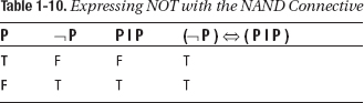
The last column of Table 1-10 shows that regardless of the truth value of P, ¬P is always logically equivalent with P|P. The proof that you can also express AND and OR in terms of NAND is left as an exercise at the end of this chapter.

The main reason why every textbook on the science of logic ends up with the five operators introduced earlier lies in the origin of this particular science: “concerning language and speech” or “human reasoning.” If you study natural languages, you’ll discover that the five operators introduced here are the ones we (human beings) use when reasoning.

Special Predicate Categories

Two predicate categories deserve a special name: tautologies and contradictions.

Tautologies and Contradictions

A tautology is a propositional form that’s TRUE for every possible combination of truth values of the propositional variables. A contradiction is a propositional form that’s false regardless of the truth values the propositional variables happen to take. Examples of tautologies are as follows:

The first example illustrates what is known in logic as “ Tertium non datur,” or the law of the excluded middle. The second example is rather obvious. The third one is TRUE regardless of the truth value of P. You can prove the last tautology using a truth table, as shown in Table 1-11.

As you can see, the last column of Table 1-11 contains only TRUE; this means that the predicate P ⇒ ( P ∨ Q ) in the corresponding column header is always TRUE regardless of the individual truth values of the variables P and Q, and therefore a tautology. Table 1-10 (expressing the NOT connective with NAND) also shows an example of a tautology.

Along the same lines, a propositional form is a contradiction if it always evaluates to FALSE, regardless of the individual truth values of its components. The following expression is a contradiction:

If you set up a truth table for this predicate, you’ll end up with only FALSE in the corresponding column. Do you think it’s obvious that the expression is a contradiction? Perhaps this example will give you some feel for the importance of being able to perform purely formal analysis on logic expressions, without regard for what the variables P and Q involved stand for.

Modus Ponens and Modus Tollens

The Modus Ponens (Latin: mode that affirms) and Modus Tollens (Latin: mode that denies) are probably the most famous examples of tautologies in logic. In regular text, they respectively read as follows:

• If P implies Q and P is TRUE, then Q must be TRUE.
• If P implies Q and Q is FALSE, then P must be FALSE.

You can also express these two tautologies using the logic operator symbols:

The Modus Ponens represents the most direct form of everyday reasoning; therefore it is also referred to as direct reasoning. The Modus Tollens is also known as indirect reasoning, a form of reasoning that’s much less familiar. Take a look at the following example.

Let P represent the predicate “Employee e is a manager” and let Q represent “Employee e earns a monthly salary of more than 10K.” Further assume that the company you work at has the following business rule: “Managers always earn more then 10K,” or, using symbols, P ⇒ Q. Indirect reasoning allows you to deduce that if you aren’t earning more than 10K monthly then you are not a manager.

Logical Equivalences and Rewrite Rules

Table 1-8 showed the truth table of the logical equivalence connective. Logical equivalences deserve our special attention because they’re extremely important, for many reasons. The most important application of logical equivalences is that you can use them to derive new equivalent predicates from existing ones; as such, they provide an alternative for using truth tables, as you’ll see in this section. They’re especially important for specifying data integrity constraints in different ways; you’ll see a lot of this in Part 2 of this book.

Setting up truth tables for complicated predicates can become quite labor intensive. For example, if the predicate you want to examine contains four proposition variables (say P, Q, R, and S), you need to set up a truth table with sixteen rows, reflecting all possible truth value combinations. You might want to use a spreadsheet to fill such a truth table efficiently once you have entered the first row, but you’ll see that using (a particular kind of) logical equivalence can be much more efficient.

Rewrite Rules

A rewrite rule is a rule that allows us to replace a given propositional form X by another propositional form Y, in such a way that X and Y are guaranteed to have the same truth value regardless of the value of the propositional variables. Such a replacement is permissible if and only if the equivalence X ⇔ Y is a tautology. This equivalence is referred to as the rewrite rule.

You already encountered an equivalence that is a tautology in the section “Functional Completeness.” It showed how implication can be expressed using a combination of disjunction and negation:

The truth table shown in Table 1-12 proves that this equivalence is indeed a tautology.

As you can see, the last column of Table 1-12 contains only TRUE. This tautology is an important rewrite rule allowing you to convert an implication into a disjunction (and vice versa). If you encounter a propositional form—or component within a propositional form—that is of the form P ⇒ Q, then you’re allowed to replace that with ¬P ∨ Q.

Table 1-12 lists the most important and well-known rewrite rules, divided in named categories. Using these rewrite rules you can replace a component (one that matches either side of a rewrite rule) in a compound predicate with some other expression (the other side of the rule) without changing the meaning of the compound predicate.

Table 1-13. Some Important Rewrite Rules

Category	Rewrite Rule
Idempotence	( P ∧ P ) ⇔ P ( P ∨ P ) ⇔ P
Double negation	P ⇔ ¬¬P
Commutativity	( P ∧ Q ) ⇔ ( Q ∧ P ) ( P ∨ Q ) ⇔ ( Q ∨ P ) ( P ⇔ Q ) ⇔ ( Q ⇔ P )
Associativity	( ( P ∧ Q ) ∧ R ) ⇔ ( P ∧ ( Q ∧ R ) ) ( ( P ∨ Q ) ∨ R ) ⇔ ( P ∨ ( Q ∨ R ) )
Distribution	( ( P ∨ Q ) ∧ R ) ⇔ ( ( P ∧ R ) ∨ ( Q ∧ R ) ) ( ( P ∧ Q ) ∨ R ) ⇔ ( ( P ∨ R ) ∧ ( Q ∨ R ) )
De Morgan Laws	¬ ( P ∨ Q ) ⇔ ( ¬P ∧ ¬Q ) ¬ ( P ∧ Q ) ⇔ ( ¬P ∨ ¬Q )
Special cases	( P ∧ TRUE ) ⇔ P ( P ∨ FALSE ) ⇔ P ( P ∨ TRUE ) ⇔ TRUE ( P ∧ FALSE ) ⇔ FALSE ( P ∧ ¬P ) ⇔ FALSE ( P ∨ ¬P ) ⇔ TRUE
Implication rewrite	( P ⇒ Q ) ⇔ ( ¬P ∨ Q )

The preceding 19 rewrite rules constitute key knowledge for a database professional. Most of these are intuitively obvious. The Distribution and De Morgan Laws might need a little more thought to see that they are in fact reasonably intuitive too. We’ll spend some more time on these rewrite rules in the first section of Chapter 3.

Rewrite rules will help you in your task of formulating queries and data integrity constraints. They are crucial for database management systems too; they allow optimizers to rewrite predicates in such a way that alternative execution plans (with possibly better performance) become available while guaranteeing the same results under all circumstances.

Using Existing Rewrite Rules to Prove New Ones

Suppose you want to investigate the following logical equivalence, to see whether it is a rewrite rule:

You could use a truth table, as shown before, but you can also use existing rewrite rules such as the ones listed in Table 1-13 to prove that this logical equivalence is in fact a tautology. Table 1-14 shows what such a proof might look like. Here we make use of the aforementioned rewrite rule that enables you to convert an implication into a disjunction and vice versa:

Table 1-14. Proving Rewrite Rules with Rewrite Rules

Input Expression	Equivalent Expression	Comment
( P ⇒ Q )	⇔ ( ( P ⇒ Q ) ∨ FALSE )	Trivial; second special case in Table 1-13
	⇔ ( ( ¬P ∨ Q ) ∨ FALSE )	Convert implication into disjunction
	⇔ ( ( ¬P ∨ ¬¬Q ) ∨ FALSE )	Double negation
	⇔ ( ¬ ( P ∧ ¬Q ) ∨ FALSE )	De Morgan
	⇔ ( ( P ∧ ¬Q) ⇒ FALSE )	Convert disjunction to implication

This completes the proof; we have derived a new rewrite rule from the ones we already knew, without using a truth table. If you look back at Table 1-7 with the definition of the implication connective, our new rewrite rule in the preceding text makes sense; it precisely corresponds with the only situation where the implication returns FALSE, also known as the broken promise.

Chapter Summary

Before continuing with the exercises in the next section, you might want to revisit certain sections of this chapter if you don’t feel comfortable about one of the following concepts, introduced in this first chapter about logic:

• A value is an individual constant with a well-determined meaning.
• A variable is a holder for a (representation of a) value.
• A proposition is a declarative sentence that is unequivocally either TRUE or FALSE.
• A predicate is a truth-valued function with parameters.
• You can convert a predicate into a proposition by providing values for the parameters or by binding parameters with a quantifier.
• You can build compound predicates by applying logical connectives to existing ones; this chapter introduced negation, conjunction, disjunction, implication, and equivalence.
• Logical connectives can be regarded as logical operators; they take one or more (input) predicates as their operands, and return another predicate as their output.
• The input predicates of a compound predicate are also referred to as the components of the compound predicate.
• The precise meaning of all logical connectives can be defined using truth tables, and you can use truth tables to investigate the truth value of compound predicates.
• A tautology is a proposition that is always TRUE, and a contradiction is a proposition that is always FALSE.
• A rewrite rule is a tautology that has the form of an equivalence.
• You can use rewrite rules to derive new rewrite rules without using truth tables.

Exercises

1. Which of these predicates are propositions?
   1. The sun is made of orange juice
   2. y + x > y
   3. There exists a database management system that is truly relational
   4. If you are not female you must be male
   5. 5 is an even number
2. Express the logical connectives AND and OR in terms of the NAND connective, as defined in Table 1-9.
3. Show that the rewrite rules in Table 1-13 are correct, by setting up a truth table for each of them or by using the rewrite rules you checked earlier during this exercise.
4. Show that the following important rewrite rules concerning the implication are correct:
   1. ( P ⇒ Q ) ⇔ ( ¬Q ⇒ ¬P )
   2. ( P ⇔ Q ) ⇔ ( ( P ⇒ Q ) ∧ ( Q ⇒ P ) )
   3. ¬ ( P ⇒ Q ) ⇔ ( P ∧ ¬ Q )
   4. ¬ ( P ∧ Q ) ⇔ ( P ⇒ ¬Q )
   5. ( ( P ⇒ Q ) ∧ ( P ⇒ ¬Q ) ) ⇔ ¬P (the absurdity rule)
5. Look at the following predicates, and check whether they are tautologies:
   1. P ⇒ ( P ∧ Q )
   2. P ⇒ ( P ∨ Q )
   3. ( P ∧ Q ) ⇒ P
   4. ( P ∨ Q ) ⇒ P
   5. ( P ∧ ( P ⇒ Q ) ) ⇒ Q
   6. ( P ⇒ Q ) ⇒ ( P ∧ Q )
   7. ( P ∧ Q ) ⇒ ( P ⇒ Q )
   8. ( ( P ⇒ Q ) ∧ ( Q ⇒ R ) ) ⇒ ( P ⇒ R )
   9. ( P ⇒ R ) ⇒ ( ( P ⇒ Q ) ∧ ( Q ⇒ R ) )
   10. ( P ∨ Q ) ⇔ ( ¬P ⇒ Q )
   11. ( P ∨ Q ∨ R ) ⇔ ( ( ¬P ∧ ¬Q ) ⇒ R )
   12. ( P ∨ Q ∨ R ) ⇔ ( ¬P ⇒ ( Q ∨ R ) )
   13. P ∨ ( Q ∧ R ) ⇔ ( ¬P ⇒ Q ) ∨ ( ¬P ⇒ R )
   14. P ∨ ( Q ∧ R ) ⇔ ( ¬P ⇒ Q ) ∧ ( ¬P ⇒ R )