This chapter is about set theory. Set theory provides an excellent language to reliably describe complex database designs, data retrieval, and data manipulation. Set theory is reliable because it is both precise and powerful; this will become clear from Chapter 5 onwards. As explained before, you’ll need to exercise some patience: Chapters 1 through 4 first lay down the foundation.

In the section “Sets and Elements,” the concepts of a set and an element of a set are introduced. In the section “Methods to Specify Sets,” you’ll see how you can specify sets using the enumerative, predicative, or substitutive method.

You probably remember your math teacher drawing pictures on the blackboard while explaining sets; the third section introduces these so-called Venn diagrams. Venn diagrams can be useful as graphical illustrations when you’re working with multiple sets. However, note that Venn diagrams are “just” pictures, just like the well-known entity-relationship diagrams are pictures that you can draw for database designs. They are often imprecise, they always leave out important details, and they can even be “misleading by suggestion.” Nevertheless, when used with caution, they can be quite helpful.

The section “Cardinality and Singleton Sets” discusses the cardinality of a set and introduces the concept of a singleton set.

Then we’ll discuss subsets and their most important properties in the section “Subsets,” followed by the well-known set operators union, intersection, and (symmetric) difference in the section “Union, Intersection, and Difference.” In the same section we’ll explore disjoint sets—that is, sets with an empty intersection.

The section “Powersets and Partitions” introduces two slightly more advanced set theory concepts: powersets and partitions. These two concepts are quite useful in database modeling, as you’ll see in later chapters.

Ordered pairs (x;y) have a first coordinate x and a second coordinate y. In the section “Ordered Pairs and Cartesian Product,” we’ll explore sets of ordered pairs and the Cartesian product of two sets. As you’ll find out in Chapter 4, we’ll use sets of ordered pairs to define (binary) relations and functions, which in turn will be used to define tables and databases—so we’re getting closer and closer to the application of the mathematics.

The section “Sum Operator” introduces the sum operator.

You’ll find a “Chapter Summary” at the end of the chapter, followed by an “Exercises” section. We strongly advise you to spend sufficient time on these exercises before moving on to other chapters.

Sets and Elements

Set theory is about sets, obviously. And there we are, faced with our first problem: what exactly is a set? A set is a collection of objects, and those objects are called the elements of the set. In mathematics, we like to be precise—so we want formal definitions of all terms we use. Just like in geometry, we all have a common understanding of what a point is, but providing a formal definition of a point turns out to be difficult. That’s why we declare them as primitive terms; that is, they are just given, and you don’t need to define them. Probably the best definition of a set is the one given by Definition 2-1.

As a rather obvious but important consequence, no two distinct sets contain the same elements; moreover:

• The elements of a set don’t have any ordering
• Sets don’t contain duplicate elements

Two sets, say A and B, are the same if each element of A is also an element of B and each element of B is also an element of A.

Note that elements of a set can be any type of object. They can even be sets on their own; you’ll see numerous examples of sets containing sets as elements in the remainder of this book.

Set theory has a mathematical symbol ∈ that is used to state that some object is an element of some set. The following expression states that object x is an element of set S:

The negation of this, saying that x is not an element of S, is expressed as follows:

This latter expression is shorthand for the negation of the former expression:

Table 2-1 lists these and some other commonly used set-theory symbols.

Table 2-1. Set-Theory Symbols

Symbol	Meaning
∈	Is an element of
∉	Is not an element of
Z	The set of all positive and negative integers, including value zero
N	The set of natural numbers; that is, integers greater than or equal to zero
∅	The empty set

N and Z are examples of sets from regular arithmetic; following are some other examples:

• The set, say P, of all prime numbers less than 20:
  P := {2,3,5,7,11,13,17,19}
• The set, say W, of the seven names of the days of the week:
  W := {'sunday','monday', 'tuesday','wednesday','thursday','friday','saturday'}

Here we use the enumerative method of specifying a set: listing all elements, separated by commas, between braces. This and some other methods of specifying a set are introduced in the next section.

The empty set symbol ∅ represents a set that has no elements. {} is also used for the representation of the empty set.

As soon as you have given your sets a name, as we did for the preceding two sets P and W, you can write expressions such as the following:

Note that the first four expressions are in fact propositions; all of them have truth value TRUE, by the way. The last one is a predicate (assuming x represents a numeric variable).

You can try to keep your expressions readable by adopting certain standards; for example, it’s common practice to use lowercase naming for elements and uppercase naming for sets. However, note that this is a naming convention only; you cannot draw any conclusions from the fact that an identifier name is spelled in uppercase or lowercase. Consider the following expression:

This expression is defined only if Y represents (or refers to) a set; otherwise, it is an undefined, meaningless, or ill-formed formula. That is, if Y doesn’t refer to a set, you cannot say whether the statement is TRUE or FALSE. On the other hand, both X and Y could refer to sets, because sets may contain sets as elements. Check out the following three examples:

3∈5 is neither TRUE nor FALSE; it is a meaningless expression

1∈{1,2} is TRUE and 2∈{1,2} is TRUE

{1,2}∈{1,2} is FALSE

{1,2}∈{{1,2},3} is TRUE

To clarify the last example being a TRUE proposition, let’s give the set at the right-hand side a name:

Then set S contains two elements: the first element is set {1,2} and the other element is the numeric value 3. Therefore, the statement {1,2}∈{{1,2},3} is a TRUE proposition.

Methods to Specify Sets

So far, you have already seen several examples of sets; with the exception of sets Z and N, they all used the enumerative method to specify their elements, listing all their elements as a comma-separated list enclosed in braces. The other methods we’ll discuss in this section are based on a given set and use predicates to derive new sets.

Enumerative Method

Enumeration (literally, to name one by one) is by far the simplest set specification method; you list all elements of a set between braces (also known as accolades) separated by commas. See Listing 2-1 for some examples.

Note that in mathematics, elements of the same set don’t need to be of the same type; for example, set E2 in Listing 2-1 contains a mixture of numbers and characters.

Note also that the order in which you specify the elements of a set is irrelevant; moreover, repeating the same element more than once is not forbidden but meaningless. Therefore, the following three sets are equal:

The disadvantage of the enumerative method to specify sets becomes obvious as soon as the number of elements of the set increases; it takes a lot of time to write them all down, and the expressions become too long.

Predicative Method

For a large set, an alternative way to specify the set is the predicative method. Let S be a given set (for instance the set of natural numbers), and let P(x) be a given predicate with exactly one parameter named x of type S (that is, the elements in S constitute the values that parameter x is allowed to take). Then, the following definition of a set, called E4, is a valid one:

This method also uses braces to enclose the set specification (just like the enumerative method) but now you specify a vertical bar symbol (|) somewhere between the braces. This vertical bar should be read as “. . . such that . . .” or “. . . for which the following is true: . . .”

At the right-hand side of the vertical bar you specify a predicate, and at the left-hand side you specify a set from which to choose values for the parameter involved in the predicate. The preceding syntax should be read as follows: “The set E4 consists of all elements x of S for which the predicate P(x) becomes TRUE.”

See Listing 2-2 for some examples of using this method (assume EMP represents some set containing “employee records,” loosely speaking). The first example uses the mod (modulo) function, which might be unfamiliar for you; it returns the remainder of division of the first argument by the second argument.

Set E5 has as its elements all even integers (zero remains after division by two) whose quadratic is less than or equal to 169. Set E6 has as its elements all employee records whose JOB value equals 'SALESREP'.

Substitutive Method

The third method to specify sets is the substitutive method. See Listing 2-3 for some examples of using this method.

The preceding specification for set E7 should be read as follows: “The set E7 consists of all x2 – 1 values where x is an element of N.” In general, the left-hand side of both set specifications (E7 and E8) now contains an expression; the right-hand side after the vertical bar tells you from which set you must choose the values for x to substitute in that expression.

Hybrid Method

Optionally, the right-hand side can be followed by a predicate that has x as a parameter. This enables you to specify set E4 also, as follows:

The left-hand side now contains just x, instead of some expression using x. Often it is convenient to use a hybrid combination of the predicative and the substitutive method for a set specification. Take a look at the example in Listing 2-4.

Formally, this is a contraction of the following specification of set E9 consisting of two steps, using an intermediate set definition T1:

T1 := { x∈N | mod(x,3) = 1 } (Using the predicative method first)

E9 := { x2 – 1 | x∈T1 } (Followed by the substitutive method)

Of course, we don’t formally split up set definitions like this. The predicative, substitutive, and hybrid methods all have in common that they allow you to use a given set and predicates in cases where using the enumerative method would become too labor intensive. For every set you want to specify, you just select the most appropriate specification method. In this book, the hybrid method will be the main method used to specify large sets.

Venn Diagrams

Venn diagrams (named after the Scottish professor John Venn) are pictures of sets. They can help you visualize the relationships between multiple sets. However, keep in mind that Venn diagrams are “just” pictures; they can also be confusing and even misleading. You probably remember Venn diagrams from the math lessons during your school days. See Figure 2-1 for Venn diagram examples showing the three sets E1, E2, and E3 from Listing 2-1.

Figure 2-1. Venn diagram examples

The Venn diagram of set E3 is already confusing, because it contains the numbers 8 and 6 twice; moreover, it isn’t immediately obvious that set E3 contains three elements. It isn’t clear how you should represent an element that is a set itself in a Venn diagram. Evidently set E3 is not suited to be represented as a Venn diagram. And if you want to investigate the empty set, you face the tough problem of how to draw an empty set in a Venn diagram. As long as you keep their limitations in mind, Venn diagrams can be quite helpful. In the rest of this chapter, they’ll be used to clarify various set-theory concepts.

Cardinality and Singleton Sets

Sets can be finite and infinite; however, when dealing with databases all your sets are finite by definition. For every finite set S, the cardinality is defined as the number of elements of S. A common notation for the cardinality of a set S is |S|, where you put the name (or specification) of the set between vertical bars. However, in this book we prefer to use the # symbol, as used in Definition 2-2, to denote the cardinality operator, because we use the vertical bar already quite heavily in predicative and substitutive set specifications.

Listing 2-5 shows some examples of sets and their cardinality.

Note the subtle difference between the first and second example. The third example shows that duplicates are not counted as separate elements; the last example shows that the set consisting of the empty set is not empty—it contains a single element, namely the empty set.

Singleton Sets

Listing 2-5 shows two examples of sets with cardinality one—the second and the last example. Sets with exactly one element are called a singleton (see Definition 2-3).

Note that a singleton is still a set; therefore, {42} is not the same as 42. {42} is a set and 42—its only element—is an integer value. Be careful; it is a common mistake to mix up a singleton set with the element it contains.

The Choose Operator

We introduce a special operator that allows you to “extract” or “choose” the single element from a singleton set. In this book we use the symbol ↵ for this operator; for example:

For singleton sets, you could consider the choose operator as an “unbracer,” enabling you to write expressions that would otherwise be somewhat more awkward. The ↵ operator always expects a singleton set as its operand; therefore, the following expression is an ill-formed, meaningless formula:

The operand here is not a singleton, but a set with a cardinality of 2.

Subsets

The concept of a subset is rather intuitive, so let’s start with the definition right away, as shown in Definition 2-4, which also introduces the reverse concept: a superset.

Note that this definition does not exclude the possibility that sets A and B are equal; the symbol we use for subsets (⊆) actually suggests this possibility explicitly. If you want to exclude the possibility of equality, you should use the special subset flavor with its corresponding symbol, as shown in Definition 2-5.

You can use the diagonal stroke as a negation; for example, A ⊄ B means that A is not a proper subset of B. Apart from this ⊄ symbol with a built-in negation, you can always use a separate negation symbol to write a logically equivalent statement, as follows:

See Listing 2-6 for some examples of propositions about subsets; check out for yourself that they are all TRUE.

The last two examples of Listing 2-6 are interesting, because they illustrate the following two important properties of subsets:

• Every set is a subset of itself: A ⊆ A
• The empty set is a subset of every set: ∅ ⊆ A

Two more subset properties worth mentioning here are the following ones:

• Transitivity: ( ( A ⊆ B ) ∧ ( B ⊆ C ) ) ⇒( A ⊆ C )
• Equality: ( A = B) ⇔ ( ( A ⊆ B ) ∧ ( B ⊆ A ) )

Union, Intersection, and Difference

You can apply various operations on sets. The most well-known set operators are union, intersection, and difference. For the difference operator, we have two flavors: the regular difference and the symmetric difference. The formal definitions and the corresponding mathematical symbols for these four operators are shown in Table 2-2.

Table 2-2. Common Set Operators

Name	Symbol	Definition
Union	∪	A ∪ B = { x | x∈A ∨ x∈B }
Intersection	∩	A ∩ B = { x | x∈A ∧ x∈B }
Difference	–	A – B = { x | x∈A ∧ x∉B }
Symmetric difference	÷	A ÷ B = ( A – B ) ∪ ( B – A )

Figure 2-2 shows corresponding Venn diagrams; the gray areas indicate the union, intersection, difference, and symmetric difference of the two sets A and B.

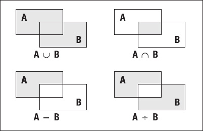
Figure 2-2. Venn diagram of the union, intersection, and difference

Let’s look at an example. Suppose the following two sets A and B are given:

Then the union, intersection, difference, and symmetric difference of A and B are as follows:

Figure 2-3 shows a Venn diagram visualizing the various areas (mentioned earlier) that correspond to the preceding expressions.

Figure 2-3. Venn diagram of A (set {1,3,5}) and B (set {3,4,5,6})

An important property of operators in general is the closure property. An operator is said to be closed over some given set, if every operation on elements of that given set always results in an(other) element of that same set.

The set operators introduced in this section always result in sets. Union, intersection, and (symmetric) difference are said to be closed over sets. The next section will discuss a few more properties of the set operators.

Properties of Set Operators

Just like we investigated various properties of the logical connectives in the previous chapter, we can do the same for set operators. Table 2-3 shows some conclusions you can draw about the properties of the four set operators.

Table 2-3. Properties of Set Operators

Property	Set Operators
Commutativity	A ∪ B = B ∪ A A ∩ B = B ∩ A A ÷ B = B ÷ A
Associativity	( A ∪ B ) ∪ C = A ∪ ( B ∪ C ) ( A ∩ B ) ∩ C = A ∩ ( B ∩ C )
Distributivity	A ∪ ( B ∩ C ) = ( A ∪ B ) ∩ ( A ∪ C ) A ∩ ( B ∪ C ) = ( A ∩ B ) ∪ ( A ∩ C )

Note that the regular difference operator is not commutative.

If you draw a Venn diagram with three sets A, B, and C, you can illustrate the associative and distributive properties of the union and the intersection intuitively (see Table 2-3), as shown in Figure 2-4.

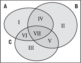
Figure 2-4. Venn diagram to illustrate associativity and distributivity

As you can see, with three sets (A, B, C) you already have seven different areas in your Venn diagram. Let’s check the following distributive property: A∩(B∪C) = (A∩B)∪(A∩C).

Set Operators and Disjoint Sets

This section explores how the set operators introduced in the previous section behave under special circumstances; namely, if the intersection of the two operands is the empty set. First, we introduce a new term to indicate that situation. See Definition 2-6 for a definition of disjoint sets.

Two sets are called disjoint if and only if they have no elements in common; that is, if and only if their intersection is the empty set. Listing 2-7 shows some properties of disjoint sets, apart from the fact that their intersection is the empty set by definition.

Set Operators and the Empty Set

As another special case, it’s always a good idea to check the behavior of the empty set, because we want it to behave just like any other set. So let’s see how the union, intersection, and difference set operators behave if the empty set is involved as one of their operands:

In other words, a union with the empty set doesn’t add anything. Every intersection with the empty set is empty because there are no common elements; the difference and the symmetric difference don’t take any elements out, so they don’t change anything either.

The following logical equivalence is also a tautology—that is, it is a rewrite rule:

You can prove this equivalence in two steps, with the following reasoning:

• If A – B is the empty set, then you can show that A is a subset of B;
• if B – A is also the empty set, then you can also show that B is a subset of A;
• but then A must be equal to B.

The proof of the other direction of the equivalence is trivial; if A and B are equal, then A – B and B – A are obviously the empty set.

Powersets and Partitions

Powersets and partitions are two more advanced set theory concepts. Let’s start with the definition of the important concept of the powerset, as shown in Definition 2-7.

Now let’s look at an example. Suppose the following two sets are given:

Then the powerset of V looks like this:

And the powerset of W looks like this:

Note that the set V itself is an element of the powerset of V, and the empty set too—which we already mentioned as being two important properties of subsets. Check for yourself that the following propositions are all TRUE, based on the same two sets V and W:

Listing 2-8 shows two properties related to powersets.

The first logical equivalence follows immediately from the definition of the powerset; the second one becomes clear if you consider that for every possible subset, each element of A can be selected as an element or can be left out—that is, for every element of A you have two choices. Therefore, if set A contains n elements, the total number of possible subsets becomes 2n ( 2 power n), the two extreme subsets being the empty set ( n times “left out”) and the set itself ( n times “selected”). See also the earlier example of set V, containing three elements ({1,2,3} ), and its powerset ℘V, containing eight elements.

The concept of a powerset is one of two key stepping stones that will be used in Part 2 of this book, when we’ll introduce the concept of a database universe as a formal definition for a database design. The second key concept, which will be introduced in Chapter 4, is the concept of a generalized product of a set function.

Union of a Set of Sets

Before we discuss the concept of partitions in the next section, we first introduce a slightly more convenient flavor of the union operator. Although the union operator is dyadic (that is, it accepts two operands), it often occurs that you want to “union” several sets, not just two; for example:

To save a lot of typing (repeating the union symbol each time), we introduce a special monadic notation (accepting only one operand) for the union operator, as shown in Definition 2-8.

You see what this definition does? The result of the union ∪A contains all elements x that occur in some set, say Ai, which is an element of A. Remember, for this definition to be valid, every element of set A must be a set.

If you look at the following examples, you’ll see that this “union of a set of sets” is indeed a more powerful and generic union operator than the dyadic one we used so far, because now you can produce the union of any number of sets with a convenient shorthand notation. In these examples, S and T represent a set:

If you don’t understand these equalities at first sight, you might want to check them against the formal Definition 2-8. Take a look at the following rather simple example; you can see that this operator acts as a “brace remover:”

Suppose: S := {{1,2,3},{2,3,4},{4,5,6}} (a set consisting of sets)

Then: ∪S = {1,2,3,4,5,6}

Partitions

Now that we’ve introduced the union of a set of sets, we can define partitions as shown in Definition 2-9.

Or, described in a more formal way, you could use the following equation:

This definition states the following:

• P is a proper subset of the powerset ℘S (because the empty set is excluded).
• Any two elements of the partition must be disjoint.
• The union of partition P must result in the original set S .

If you want to think in terms of Venn diagrams, a partition is simply a matter of segmenting the original set in a number of non-empty non-overlapping pieces, as illustrated in Figure 2-5. Suppose S := {1,2,3,4,5,6,7,8,9} and P := {{1},{2,4},{3,6,7},{5},{8,9}} . Then every element of S occurs in precisely one element of partition P.

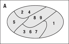
Figure 2-5. Venn diagram of partition P

Let’s look at another rather simple numeric example:

Suppose: T := {1,2,3}

Then the sets P1 through P5 are all the possible partitions of T:

Note that the last example shows that in general {S} is always a partition of S. Always? Even if S is the empty set? Check this statement carefully against the definition of a partition; this check is left as an exercise at the end of this chapter.

Ordered Pairs and Cartesian Product

If a set contains two elements, the order of those two elements is irrelevant. For example, the set {1,2} is identical to the set {2,1}. On the other hand, in geometry we normally represent points with x and y coordinates, where the order of the coordinates is important. If you swap the x and y coordinates of a given point, assuming they are not the same value, you end up with a different point.

Ordered Pairs

This section introduces the concept of ordered pairs, allowing you to make the distinction in the order of two values that are paired together. We use a special notation for this, as shown in Definition 2-10.

The concept of an ordered pair is important in this book. That’s not only because we’ll use ordered pairs to introduce the Cartesian product operator; but moreover, we will need them to introduce binary relations and functions in Chapter 4, which in turn will be used to represent tuples (we note now that this word is pronounced such that it rhymes with “couples”).

The two elements of an ordered pair are also referred to as the first and second coordinates of the ordered pair. Because the order of the coordinates of an ordered pair is important, the following two properties hold:

The second property in the preceding equation is also known as the “equality axiom.” Using De Morgan’s rewrite rules you can also specify this axiom as follows:

We introduce operators π₁ and π₂ to retrieve the first and second coordinates from an ordered pair. For a given ordered pair—say (a;b)—the first coordinate can be retrieved using the expression π₁(a;b), which results in a, and the second coordinate via expression π₂(a;b), which equals b.

Cartesian Product

The Cartesian product of two given sets can now be defined using ordered pairs, as shown by Definition 2-11.

That is, the Cartesian product A×B is the set of all ordered pairs you can construct by choosing a first coordinate from set A and a second coordinate from set B. Let’s look at an example. Suppose the following sets are given:

Then

And

This example clearly shows that A×B is in general not the same as B×A. In other words, the Cartesian product operator is not commutative. You can even prove that in case A×B and B×A are the same, A and B must be equal (and vice versa):

Note also that the two example sets A and B contain numbers as their elements, while the results of both Cartesian products contain ordered pairs. In this regard, the Cartesian product clearly differs from the operators we discussed before. The union, intersection, and difference operators all repeat (or leave out) elements of their operands; they don’t create new types of elements.

Because the Cartesian product produces every possible combination of two coordinates from the two finite input sets, the following property is also rather intuitive (also see the preceding example):

The cardinality of a Cartesian product is equal to the product of the cardinalities of the two operands. Last but not least, let’s not forget to check the empty set:

Sum Operator

We conclude this introductory chapter on set theory by establishing the sum operator (see Definition 2-12). With the sum operator, you can evaluate a numeric expression for every element in a given set and compute the sum of all these evaluations.

Here are a few examples:

The first example sums values -1, 2, and 5. This results in 6. The second example is a somewhat elaborate way to compute the cardinality of the set {-1,2, 5 }; it sums value 1 for every element in this set and results in 3. The third example computes the sum 2*0 + 2*1 + 2*2 + 2*3 + 2*4 and results in 20. The fourth example computes 1 + 1 + 5, resulting in 7.

Some Convenient Shorthand Set Notations

We use some (finite) sets frequently in the database world: dates, numbers, and strings. Therefore, we introduce the set specification shorthand listed in Table 2-4.

Table 2-4. Some Convenient Set Specification Shorthand

Shorthand	Definition
date	{ d | d is a date between January 1, 4712 BC and December 31, 4712 AD }
number(p,s)	{ n | n is a valid number with precision p and scale s }
varchar(n)	{ s | s is a string with at least 1 and at most n characters }
[n..m]	{ x∈Z | x ≥ n ∧ x ≤ m }

As you can see, this shorthand shows a rather obvious resemblance with the common data types that are supported by SQL database management systems. For the date shorthand, the boundaries defined are those that are implemented by at least one common DBMS vendor. The last shorthand in Table 2-4 allows you to specify closed intervals of integers.

Chapter Summary

This section provides a summary of this chapter, formatted as a bulleted list. You can use it to check your understanding of the various concepts introduced in this chapter before continuing with the exercises in the next section.

• Sets are fully characterized by their elements and nothing but their elements.
• You can specify sets by enumeration, by using the predicative method, by using the substitutive method, or a mixture of the predicative and substitutive methods.
• Venn diagrams are pictures of sets, and as such can provide a visual aid when working with sets; however, keep their limitations in mind.
• The number of elements of a finite set is known as its cardinality. We use the symbol # to represent the cardinality operator.
• A set with precisely one element is known as a singleton; for singletons we can use the “choose” operator (↵) to unpack the singleton element.
• A is a subset of B if every element of A is also an element of B; the notation is A⊆B. If A is also not equal to B, it is called a proper subset of B (the notation is A⊂B ).
• Every set is a subset of itself, and the empty set is a subset of every set.
• The most common set operators are union, intersection, and (symmetric) difference.
• Two sets are called disjoint if their intersection is the empty set.
• The powerset ℘V of a set V is the set consisting of all possible subsets of V. If V contains n elements, then the powerset ℘V contains 2n elements (including the empty set and V itself).
• The union of a set of sets is a generalization of the dyadic union operator, allowing you to produce the union of an arbitrary number of sets.
• A partition of a non-empty set S is a set of mutually disjoint, non-empty subsets of S for which the union equals S .
• An ordered pair (a;b) consists of two coordinates, a and b, for which the order is important; in other words, ( (a;b) = (c;d) ) ⇔ ( a = c ∧ b = d ).
• The π₁ and π₂ operators enable you to retrieve the first and second coordinates from an ordered pair.
• The Cartesian product of two sets is the set consisting of all possible ordered pairs you can construct by choosing a first coordinate from the first set and a second coordinate from the second set.
• The sum operator enables you to compute the sum of a given expression across a given set.

Exercises

1. Suppose the following set is given: A := {1,2,3,4,5 }

   Which of the following expressions are TRUE?

   1. 3 ∈ A
   2. 3 ⊂ A
   3. ∅ ⊆ A
   4. ∅ ∈ A
   5. {2} ⊂ A
   6. {3,4} ∈ A
   7. {3,4} ⊂ A
   8. {{3,4}} ⊄ A
   9. #{{3,4}} = 2
   10. ∅ ∈ {∅}
   11. ∅ ⊂ ∅
   12. ∅ ∈ {0}
   13. {1,2,3,∅} = {1,2,3}
2. Give an enumerative specification of the following sets:
   1. { 2x - 1 | x ∈ N ∧ 1 < x < 6 } = ...
   2. { y | y ∈ N ∧ y = y+1 } = ...
   3. { z | z ∈ N ∧ z = 2*z } = ...
3. Give a formal (predicative) specification for the following sets:
   1. The set of all quadratics of the natural numbers
   2. The set of all even natural numbers
   3. The set of all ordered pairs with natural number coordinates such that the sum of both coordinates does not exceed 10
4. Draw a Venn diagram of the following three sets:
   A := {1,2,4,7,8}
B := {3,4,5,7,9}
C := {2,4,5,6,7}

   Enumerate the elements of the following set expressions:

   1. B ∪ ∅
   2. B ∪ {∅}
   3. A – (B – C )
   4. ( A – B ) – C
   5. B ÷ C
   6. A – B ∩ C
5. Which of the following seven sets are equal?
   A := ∅
B := {0}
C := {∅}
D := {{∅}}
E := { x∈N | x = x+1 }
F := { x∈N | x = 2x }
G := { x∈N | x = x2 }
6. Suppose the following set is given:
   S := {1,2,3,{1,2},{1,3}}

   Which of the following expressions are TRUE?

   1. {1,2} ⊂ S
   2. {1,2} ∈ S
   3. {1,2} ∈ ℘S
   4. {2,3} ⊂ S
   5. {2,3} ∈ S
   6. {2,3} ∈ ℘S
   7. {1} ∉ ℘S
   8. {∅,S} ⊆ ℘S
   9. {∅} ∈ ℘℘S
   10. #℘℘S = 25
   11. ∪S = {1,2,3}
   12. {{1,2,3},{{1,2}},{{1,3}}} is a partition of S

       Evaluate the following set expressions:

   13. #S = ...
   14. { x∈ ℘S| #x = 2 } = ...
   15. S – ∅ = ...
   16. ∅ – S = ...
   17. S ∩ ∅ = ...
7. Continuing with the example set S of the previous exercise, which connection symbols can you substitute for the ellipsis character ( ... ) in the first column of the following table, in such a way that it becomes a TRUE proposition?

   

   

8. Suppose you have three sets A, B, and C, satisfying the following conditions:
   #(A∩B) = 11
#(A∩C) = 12
#(A∩B∩C) = 5

   What is the minimum cardinality of set A?

9. The following two sets are given:
   S := {1,2,3,4,5}
T := {6,7,{6,7}}

   Evaluate the following expressions:

   1. ∪{S,T} = ...
   2. ℘S – S = ...
   3. ℘T – T = ...
   4. T– ℘ T = ...
   5. #∪℘S = ...