C H A P T E R  13

Performance Tuning and Optimization

SQL Server 2012 and the Windows operating systems that it runs on perform very well storing, maintaining, and presenting data to your users. Many of the processes that make them run so well are built into SQL Server 2012 and the operating system. Sometimes, because of a variety of factors, such as data changes, new code, or poor design choices, performance can suffer. To understand how well, or poorly, your server is performing, you need to understand how to measure that performance.

A number of methods of collecting performance data are available, including the Performance Monitor utility in Windows and the dynamic management objects (DMOs) in SQL Server. All this server information can be automatically collected through the use of a utility built into SQL Server 2012, the data collector. But understanding how the server is performing is not enough. You also need to know how the queries running on the server are performing. You can gather this information using Extended Events sessions. Once you know which queries or processes are running slowly, you’ll need to understand what’s going wrong with them. Again, SQL Server provides a tool—execution plans, which allow you to look into the functions within a query. If you really need help with performance, another automated utility called the Database Tuning Advisor can help.

If this topic sounds large, it is. Entire books have been written about tuning the server and queries. This chapter will act as an introduction to the various mechanisms of performance monitoring and the processes available for tuning and optimizing performance. Some tools, such as the Resource Governor and data compression, can even help you automatically control performance on your server. The Resource Governor will help prevent any one process from consuming too many of the limited resources available on a server. Data compression will automatically make your data and indexes smaller, using fewer resources and, in some cases, speeding up the server.

Measuring SQL Server Performance

The metrics necessary to understand how your server is performing can be grouped into four basic areas: memory, central processing unit (CPU), disk input/output (I/O), and network. When your server is running slowly, one of these four elements needs tuning. To gather the information about these processes, and many more besides, the Windows operating system exposes what are called performance counters for your use. There are three ways to look at performance counters: using the Performance Monitor utility, using DMOs, and using the Data Collector.

Understanding Performance Counters

Before getting into the methods to look at performance counters, we’ll discuss which performance counters are most useful to you. When you see the list of available performance counters, you’re likely to be overwhelmed. Table 13-1 describes the most commonly used and useful performance counters, what they measure, and what represents potentially problematic measurement. Performance counters are grouped together by what are referred to as objects. Objects may have a particular application called an instance. Under this are the actual counters. To present the information, the Object(Instance):Counter format is usually used.

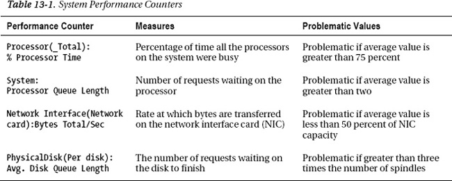
These basic counters will show you the amount of time that the various system processes are spending working on your system. With the queue length of the processor and the disk, you can see whether some processes are waiting on others to complete. Knowing that a process is waiting for resources is one of the best indications you’ll get that there is a performance problem. You can also look at the amount of information being sent over your network interface card (NIC) as a general measure of problems on your network. Just these few simple counters can show you how the server is performing.

To use these counters, you need a general idea of what constitutes a potential problem. For example, % Processor Time is problematic when a sustained load is 75 percent or greater. But you will see occasional spikes of 100 percent. Spikes of this nature are a problem only when you also begin to see the Processor Queue Length value grow. Understanding that the Average Disk Queue Length value is growing will alert you to potential problems with I/O, but it will also let you know that your system is beginning to scale and that you may need to consider more, or different, disks and disk configurations.

Several counters will show you the performance and behavior of SQL Server itself. These are available in the same places as the system counters, but as you’ll see in Table 13-2, they are formatted slightly differently. You’ll see these as SQL Server:Object(Instance):Counter.

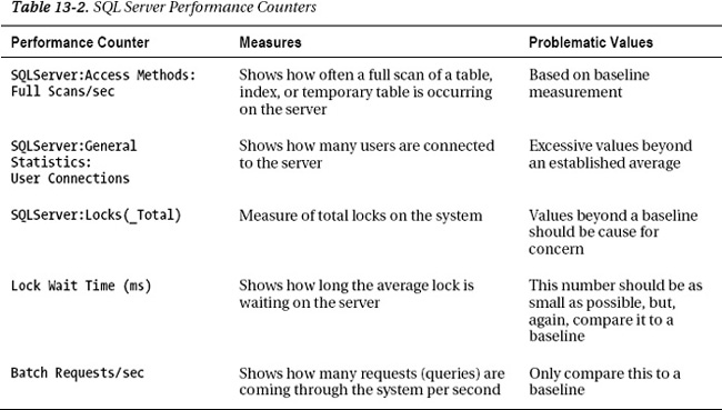
The first counter listed in Table 13-2, Full Scans/sec, lets you know how many full scans (a complete read of an index or a table row by row) the system is experiencing. Large numbers here indicate poorly written queries or missing indexes. The second counter, User Connections, simply shows the number of user connections in the system. This is useful when combined with other measures to see how the server is behaving. Lock Wait Time is an indication that a lot of activity is occurring on the server and processes are holding locks that are necessary to manipulate data. This may suggest that transactions are running slowly. Finally, the counter Batch Requests/sec indicates just how much load the server is operating under by showing the number of requests in the system.

The counters displayed in Tables 13-1 and 13-2 are a very small subset of the total counters available, but these will give you a general indication of the health of your server. You would need to look at a number of other counters to get an accurate measure of a system’s health. The counters mentioned here are the ones that are most likely indicative of a problem on the system. The idea here is that anything that is causing queuing, in other words, waits in the CPU or I/O, is a problem that needs to be identified and dealt with. Within SQL Server, growing numbers of scans or lock waits can also indicate deteriorating performance. So, although these counters won’t provide an overall health for the system, they do act like a check on the pulse of the system, which is an early indicator of other problems. There are multiple ways to access these counters on your systems.

Performance Monitor

The Performance Monitor tool comes installed with all versions of the Windows operating system. This tool provides a graphical interface for accessing the performance counters introduced in the preceding section. The easiest way to access the Performance Monitor tool, often referred to as Perfmon because of the name of the executable file, is to click the Start menu on your server and click the Run icon. Type perfmon, and then click the OK button. This will open a window that looks like Figure 13-1.

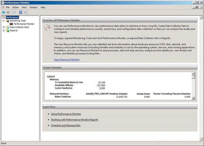
Figure 13-1. Performance Monitor suite

A number of tasks are possible with the Perfmon tool, including viewing performance monitor counters, creating logs of counters, and scheduling the capture of counters to files that can then be viewed through the Perfmon tool or imported into databases for more sophisticated data manipulation. I’ll simply show how to view a few of the counters introduced in the previous section.

You first have to access the Performance Monitor tool. Click the icon on the left side of the screen labeled Performance Monitor. This will display a screen similar to Figure 13-2.

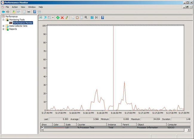
Figure 13-2. Initial Performance Monitor window

To add counters to the Performance Monitor window, click the plus icon near the center of the toolbar at the top of the window. This will open the Add Counters window, shown in Figure 13-3.

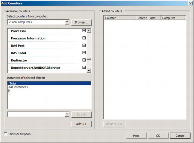
Figure 13-3. The Add Counters window in Perfmon

To select counters for a particular computer, you’ll need to supply the name of the computer in the “Select counters from computer” combo box, or you can simply let the tool select from the local computer, as displayed in Figure 13-3. To supply the name, you can either type it or select from a list of computers on your network. Once that’s done, you’ll need to select one of the performance objects. As shown in Figure 13-2, the % Processor Time object has already been selected for you. To select additional counters, scroll within the “Available counters” window. For this example, select the object General Statistics, which will have your server’s instance name in front of it so that it would read ServerInstance:General Statistics if you used the example name from Chapter 2. Scroll down until you find the User Connections counter, and then click it. Click the Add button to add this counter to the “Added counters” list on the right. When you’re done adding counters, click the OK button.

Now the Perfmon window will show activity from the two counters selected. The window shows a set period of time, and you can see the variations in data across the period, as shown in Figure 13-4.

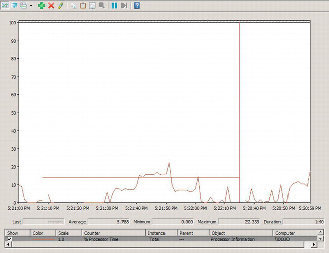
Figure 13-4. Perfmon displaying performance counters and activity

Looking at the screen displayed in Figure 13-4, you can see how the performance counters change over time. The data is collected and aggregated so that you can see important information such as the Last, Average, Maximum, and Minimum values. The duration, the amount of time on display, is also shown. You can see the list of counters that is currently on display. You can even highlight a counter by selecting it in the list and then clicking the lightbulb icon in the toolbar at the top of the screen.

With the Perfmon tool, you can further manipulate the display to show different types of graphs or raw data and change the properties of the counters displayed to adjust the color they’re displayed in or the scale on which they display. You can also choose to have the Perfmon tool output to a log. There are other ways to get at performance counters, and one of them is within SQL Server using T-SQL.

Dynamic Management Objects

Introduced in SQL Server 2005, dynamic management objects (DMOs) are mechanisms for looking into the underlying structures and processes of the SQL Server 2012 system and, to a lesser degree, into the operating system. Of particular interest for looking at performance counters is the dynamic management view (DMV) sys.dm_os_performance_counters. This shows a list of SQL Server performance counters within the results of a query. It does not show the operating system performance counters. The performance counters for the operating system are not as easily queried as are those for SQL Server. Querying sys.dm_os_performance_counters is as simple as querying a table:

This query will return all the performance counters at this instance in time. To see a specific counter or instance of a counter, you just need to add a WHERE clause to the query so that you return only the counter you’re interested in, like this:

This will return a data set similar to that shown in Figure 13-5.

Figure 13-5. Results from query against sys.dm_os_performance_counters

The column, cntr_value, shows the value for the counter being selected. If there were no other operations on the server and you were to run the query again, in this instance the counter would go up by 1 to become 44974 because even the query against the DMV counts as a batch request. Other values for other counters may go up or down or even remain the same, depending on what each of the counters and instances is recording. You can use this data in any way you like, just like a regular T-SQL query, including storing it into a table for later access. The main strength of the sys.dm_os_performance_counters DMV is that you can access the data in T-SQL and use the data it displays with the T-SQL tools that you’re used to using.

Performance counters are not the only way to tell what is occurring within SQL Server. Another method of looking at performance data is the plethora of other DMOs. Detailing all the possible details for information that you could collect through queries against DMOs is beyond the scope of the book. The DMVs within SQL Server can be roughly grouped as either server DMOs or database DMOs. There are 17 different divisions of DMOs. We won’t list them all, but we will list the groups directly used to access performance data about the system or the database:

• Database: These are primarily concerned with space and the size of the database, which is important information for understanding performance.
• Execution: The DMVs and dynamic management functions (DMFs) in this group are very much focused on the performance and behavior of the queries against the database. Some of these will be covered in the section “Tuning Queries.”
• Index: Like the database-related DMOs, these are mostly about size and placement, which is useful information. You can also track which indexes are used and whether there are missing indexes.
• I/O related: These DMOs are mainly concerned with the performance of operations against disks and files.
• Resource Governor: These DMOs are not directly related to performance but are a means of addressing the settings, configuration, and behavior of the Resource Governor, which is directly related to performance. This is covered in detail in the section “Limiting Resource Use.”
• SQL Server operating system:  Information about the operating system, such as memory, CPU, and associated information around the management of resources is available to the DMVs and DMFs grouped here.
• Transaction: With the DMOs in this group, you can gather information about active transactions or completed transactions, which is very useful for understanding the performance of the system.

The ability to query all this information in real time or to run queries that gather the data into permanent tables for later analysis makes these DMVs a very important tool for monitoring the performance of the system. They’re also useful for later tuning that performance because you can use them to measure changes in behavior. But real-time access to this data is not always a good idea, and it doesn’t let you establish a baseline for performance. To do this, another way to collect performance data is needed. This is the Data Collector.

Data Collector

Introduced with SQL Server 2008, the data collector is a means of gathering performance metrics, including performance counters, from multiple SQL Server systems (2008 and above) and collecting all the data in one place, namely, the management data warehouse. The data collector will gather performance data, including performance counters, procedure execution time, and other information. Because it exposes a full application program interface (API), you can customize it to collect any other kind of information that you want. For our purposes, we’ll focus on the three default collections: Disk Usage, Query Activity, and Server Activity.

The data collector is a great way to look at information over a long period of time so that you can provide information for tuning purposes. For example, you would want to start collecting data on a new application right away. This initial set of data is known as a baseline. It gives you something to compare when someone asks you whether the system is running slowly or whether the databases are growing quickly. You’ll also have the ability to collect performance data before and after you make a change to the system. So if you need to know whether adding a new index, changing a query, or installing a hotfix changed the performance in the system, you’ll have data collected that allows you to compare behavior before and after the change you introduced to the system. All of this makes the data collector a vital tool in your performance-monitoring and tuning efforts.

Setting Up the Data Collector

To begin using the data collector, you need to first establish security, a login, that will be used on all your servers for collecting data. You can approach this in two basic ways. First, you can have a single login across all your servers that have sysadmin privileges, which allows the login to do anything. Second, you can use the built-in data collector roles that are stored in the msdb system database. Detailing all the variations for setting up security for the data collector is beyond the scope of this book. For details, refer to “Data Collector Security” in Books Online.

Once the security is set, you’ll need to establish a server as the host to the management data warehouse, where the performance data gathered through the data collector will be stored. When you have the server ready, open SQL Server Management Studio (SSMS), and connect to the server. Scroll down the folders available in the Object Explorer window to the Management folder. Expand this. It should look something like Figure 13-6, although if you haven’t configured it, you may see a small red arrow like the one visible on the Resource Governor icon.

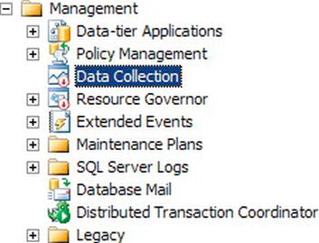
Figure 13-6. The Data Collector tool inside the Management folder

Once you have navigated to the Data Collector icon, as shown in Figure 13-6, you can begin to establish the management data warehouse. Right-click the Data Collector icon, and select Configure Management Data Warehouse from the context menu. This will open the welcome screen to the Configure Management Data Warehouse Wizard. Click the Next button to get past that screen, as shown in Figure 13-7.

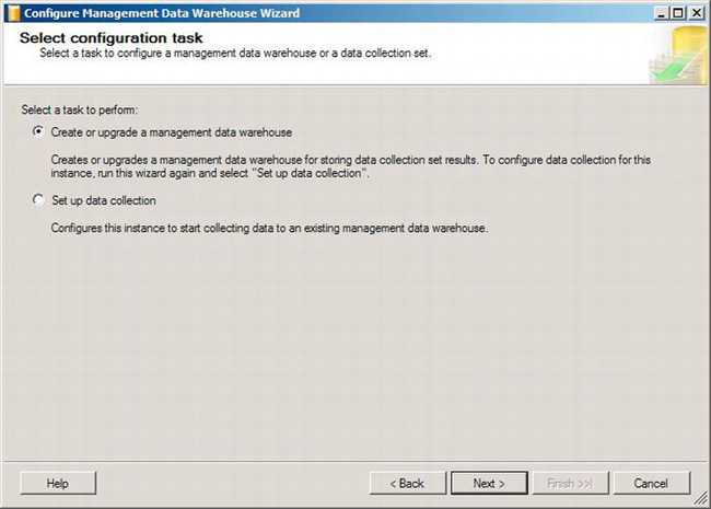
Figure 13-7. Management Data Warehouse Wizard’s “Select configuration task” page

The default behavior is to create or upgrade a management data warehouse, which is exactly what needs to happen. The other option is to set up data collection on the server that you run this on. This is how you would set up the data collector, and there will be more on that later in this section. Click the Next button. This will open the next page of the wizard, shown in Figure 13-8.

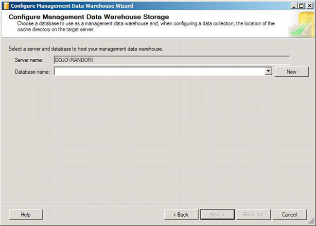
Figure 13-8. Management Data Warehouse Wizard’s Configure Management Data Warehouse Storage page

This process is very simple. Either you select an existing database to act as the management data warehouse, or you click the New button to create one when the standard Create Database window opens. Which you do depends on your system. We strongly advise against placing the data collected for the management data warehouse into one of your online transactional systems. You could place it into an existing reporting or management system. If you choose to select a new database, another window, called Map Logins and Users, will open for setting up security. Adjust this as needed for the security within your system and finish the wizard. That’s the entire process. Behind the scenes, more occurred than you can immediately see. Inside the database you selected or created, several tables were created that are used by the process to manage the collection and store the data. Stored procedures, views, user-defined functions, and other objects were also added to the database. All these objects are used to gather and present the data as it comes in from the various servers where you’ve enabled the data collector.

To configure the servers that will send their information to the management data warehouse, connect to those servers through SSMS. Navigate to the Management folder so that you can see the data collector, just like in Figure 13-6. Right-click and select Configure Management Data Warehouse from the context menu. This will again open the wizard’s welcome screen. Click Next. This will open the Select Configuration Task page like in Figure 13-7. Click the radio button “Set up data collection,” and click Next. This will open the Configure Management Data Warehouse Storage page, shown in Figure 13-9.

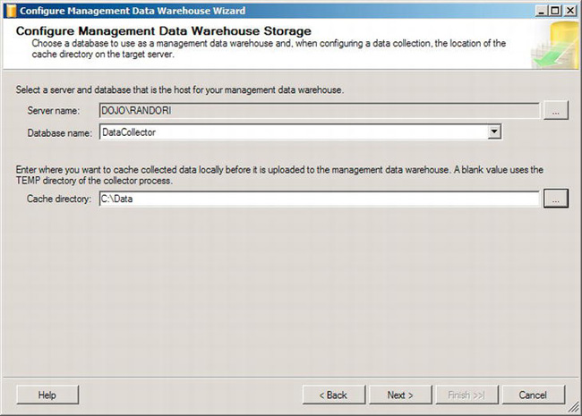
Figure 13-9. Configure Management Data Warehouse Storage page

From the server where you want to collect data, you must define the server where the management data warehouse is stored. Select the server by clicking the ellipsis button, which will enable the “Database name” drop-down. Make sure you select the database that you created previously. Finally, you need to define a directory for data to be cached while it waits for the process to pick it up for storage. Choose an appropriate location on your system. The default is to place it on the system drive (usually C:). Depending on your environment, this is probably a poor choice. Instead, a storage collection that you can manage that won’t affect other processes is a more appropriate location. The data collector is now configured and running.

Viewing the Data Collector Data

The data collector is now running on the server where you designated it. It’s collecting the data and storing it in the cache directory you defined. To start to view this data, you need to first get it from the cache directory to the management data warehouse. All the collection jobs are set up and running, but they’re not transmitting the data collected, and this transmission must be started. Initially, you can do this manually. Later, you may want to set up scheduled jobs through the SQL Agent to gather the data collector data. To get the data manually, right-click any of the defined data collection sets, and choose Collect and Upload Now from the context menu. This will take the data from the disk cache and load it into the management data warehouse. It’s now ready for viewing. You should perform this step if you’re following along to have data visible in the next steps.

The data is available in standard tables, so you could access it directly through SQL queries if you wanted. However, the data collector comes installed with a few standardized reports. If you right-click the data collector icon in the Object Explorer window, you can select Reports from the context menu and then select Management Data Warehouse from there. With the default install, three reports are available:

• Server Activity History
• Disk Usage Summary
• Query Statistics History

Server Activity History

If you select the first item in the list, Server Activity History, you’ll see a window with a number of charts. All this information represents basic server-level data, showing information such as the amount of CPU or memory used, what processes are waiting when running inside SQL Server, and the aggregated number of activities over time. All of this information is very useful for performance monitoring and tuning. There are so many charts that we can’t show them all in a single figure. The top half of the report will look like Figure 13-10.

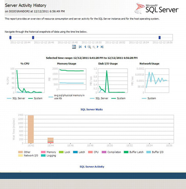
Figure 13-10. Server Activity History report, top section

At the top, you can see which server the data is being displayed for. Below that is the time period for which the data is being displayed, and you can modify or scroll through the various time periods using the controls provided. As you change the time period, the other graphs on the chart will change. Immediately below the controls, the time range currently selected is displayed. In the case of Figure 13-10, it’s showing a time range between “4/24/2009 2:00AM” and “4/24/2009 6:00AM.”

Next are a series of graphs showing different information about the system. Each graph, where appropriate, shows information about the operating system and SQL Server, color-coded as green and blue, respectively. These graphs are nice, but if you need detailed information, you need to click one of the lines. Figure 13-11 shows the detail screen for the % CPU for the system.

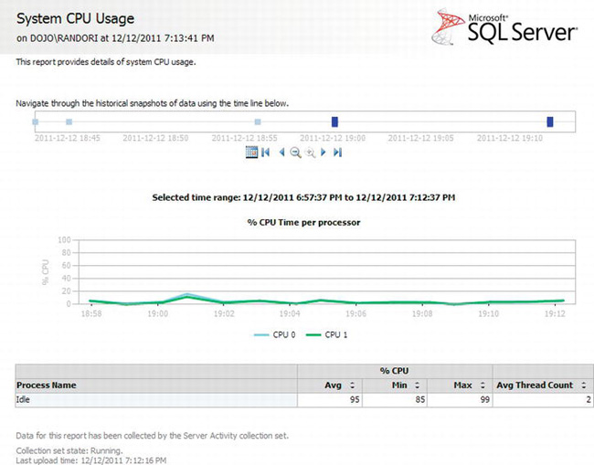
Figure 13-11. % CPU Time per processor details report

You can see that once more you have the ability to change the time frame for the report. It also displays a nice graph, even breaking down the behavior by CPU and, finally, showing aggregate numbers for % CPU over the time period. Each of the separate graphs in the main window will show different detail screens with more information specific to that performance metric. To navigate back to the main report, you click the Navigate Backward button located near the top of the window.

Back on the main window of the Server Activity History report, the bottom half of the report looks like Figure 13-12.

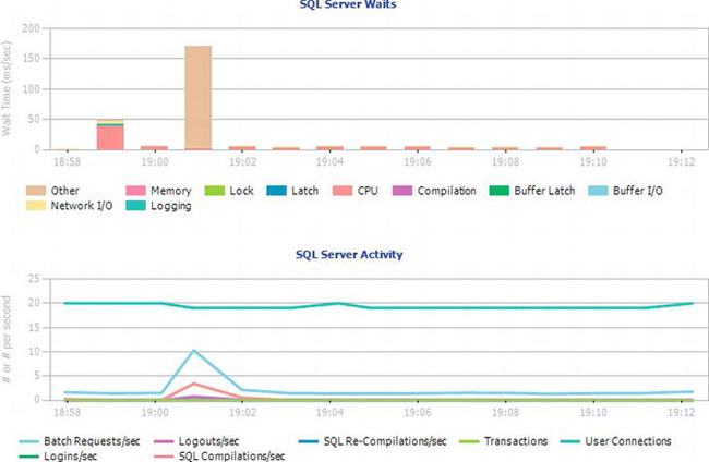
Figure 13-12. Server Activity History report, bottom section

Once again, these are incredibly useful reports all by themselves, showing the SQL Server waits broken down by wait type and showing SQL Server activity broken down by process type. With either of these reports, it is possible, as before, to select one of the lines or bars of data and get a drill-down menu showing more information.

Disk Usage Summary

When you open the Disk Usage Summary report, you see a single graph. The report lists the databases over a period when the data collector was gathered. This allows you to see how the sizes of the databases are changing over time. Figure 13-13 shows the Disk Usage Summary report.

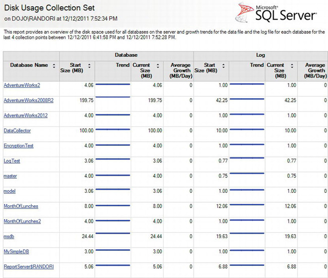
Figure 13-13. Disk Usage Summary report

As you can see, the information is laid out between the data files, shown as the database sizes, and the transaction log, shown as the log sizes. Each one shows a starting size and the current size, which allows you to see a trend. Running this report once a week or once a month will quickly let you know which databases or logs you need to keep an eye on for explosive growth.

You can click the database name to open a new report, the Disk Usage for Database report, as shown in Figure 13-14.

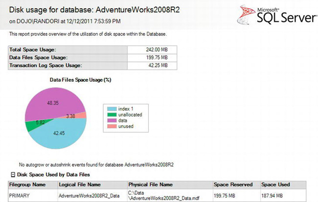
Figure 13-14. Disk Usage for Database report

The Disk Usage for Database report details how much of the space allocated to the database is being used and how much is free. It also shows whether the space used is taken up by indexes or data.

Query Statistics History

The most common source of performance problems in SQL Server is poorly written code. Gathering information on the performance metrics of queries is a vital part of performance monitoring and tuning. Opening the Query Statistics History report will display a window similar to Figure 13-15.

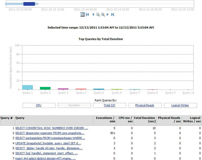
Figure 13-15. Query Statistics History report

At the top of the report is the (by now familiar) time control so that you can determine the time period you’re interested in viewing. The graph shows queries ordered by different criteria, such as CPU, Duration, Total I/O, Physical Reads, and Logical Writes. Clicking any one of these will change the display to show the top ten queries for that particular metric. In Figure 13-15, Duration has been selected, so the queries are ordered by the total duration of the query for the time period selected. This ability makes this tool incredibly useful because each of these metrics represents a possible bottleneck in your system. So, you may be seeing a number of waits on your system on the CPU in the Server Activity History report. If you then open the Query Statistics History report and sort by CPU, you can see the top ten worse offenders and begin to tune the queries (query tuning is covered in a later section called “Tuning Queries”).

Clicking one of the queries will open the Query Details report, shown in Figure 13-16. At the top of the report is the text of the query. Depending on what was run inside the query, this can be quite long. Figure 13-16 shows only the bottom half of the report.

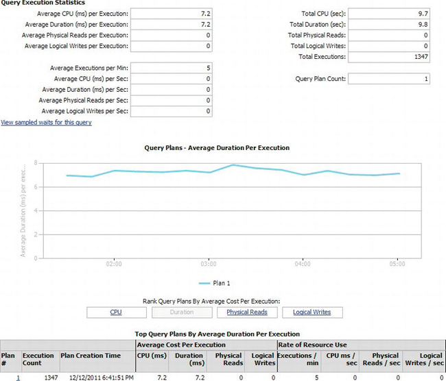
Figure 13-16. Query Details report, bottom half

The Query Details report shows a lot of information about the query selected. Starting at the top of Figure 13-16, you can see the Query Execution Statistics area. This includes various information such as the average CPU per execution, the average executions per minute, or the total number of executions for the time period. All this information provides you with details to enable you to understand the load that this particular query places on the system. The graph in the middle of Figure 13-16 shows data about the different execution plans that have been created for this query. Selecting each of the different rankings will reorder the execution plans just as it did the queries in the Query Statistics History report. Execution plans are the way that SQL Server figures out how to perform the actions you’ve requested in the query. They’re covered in more detail in the section “Understanding Execution Plans.” Being able to look at the information in the Query Details report for a query and compare it to previous entries will be a powerful tool when you begin to tune queries.

Tuning Queries

Tuning SQL Server queries can be as much of an art as a science. However, you can use a number of tools and methods to make tuning your queries easier. The first thing to realize is that most of the time, when queries are running slowly, it’s because the T-SQL code within them is incorrect or badly structured. Frequently, queries run slowly because a well-written query is not using an index correctly or an index is missing from the table. Sometimes, you even run into odd bits of behavior that just require extra work from you to speed up the query.

Regardless of the cause of the performance problem, you’ll need a mechanism to identify what is occurring within the T-SQL query. SQL Server provides just such a mechanism in the form of execution plans. You’ll also need some method of retrieving query performance data and other query information directly from SQL Server. You can capture query execution times using Extended Events. You may not have the time to learn all the latest methods and tricks for tuning your system, but you’re going to want it tuned anyway. This is where the Database Tuning Advisor comes in. These three tools—execution plans, Extended Events, and Database Tuning Advisor—provide the means for you to identify queries for tuning, understand what’s occurring within the query, and automatically provide some level of tuning to the query.

Understanding Execution Plans

There are two types of execution plans in SQL Server: estimated and actual. Queries that manipulate data, also known as Data Manipulation Language (DML) queries, are the only ones that generate execution plans. When a query is submitted to SQL Server, it goes through a process known as query optimization. The query optimization process uses the statistics about the data, the indexes inside the databases, and the constraints within and between the tables in SQL Server to figure out the best method for accessing the data that was defined by the query. It makes these estimates based on the estimated cost to the system in terms of the length of time that the query will run. The cost-based estimate that comes out of the optimization process is the estimated execution plan. The query and the estimated execution plan are passed to the data access engine within SQL Server. The data access engine will, most of the time, use the estimated execution plan to gather the data. Sometimes, it will find conditions that cause it to request a different plan from the optimizer. Either way, the plan that is used to access the data becomes the actual execution plan.

Each plan is useful in its own way. The best reason to use an estimated plan is because it doesn’t actually execute the query involved. This means that if you have a very large query or a query that is running for very excessive amounts of time, rather than waiting for the query to complete its execution and an actual plan to be generated, you can immediately generate an estimated plan. The main reason to use actual plans is that they show some actual metrics from the query execution as well as all the information supplied with the estimated plan. When the data access engine gets a changed plan, you will see the changed execution plan, not the estimated plan, when you look at the actual execution plan.

There are a number of possible ways to generate both estimated and actual execution plans. There are also a number of different formats that the plans can be generated in. These include the following:

• Graphical: This is one of the most frequently used execution plans and one of the easiest to browse. Most of the time, you’ll be reading this type of execution plan.
• XML: SQL Server stores and manipulates its plans as XML. It is possible for you to get to this raw data underneath the graphical plan when you need to do so. By itself, the XML format is extremely difficult to read. However, it can be converted into a graphical plan quite easily. This format for the execution plan is very handy for sending to coworkers, consultants, or Microsoft Support when someone is helping you troubleshoot bad performance.
• Text: The text execution plans are being phased out of SQL Server. They can be easy to read as long as the plan is not very big, and they are quite mobile for transmitting to others. However, since this format is on the deprecation list for SQL Server, no time will be spent on it here.

The easiest and most frequently used method for generating a graphical execution plan is through the query window in SQL Server Management Studio. Open Management Studio, connect to your server, and right-click a database. From the context menu, select New Query. A new query window will open. For this example, we’re using Microsoft’s test database, AdventureWorks2008R2. Type a query into the window that selects from a table or executes a stored procedure. Here’s the query we’re using (salesquery.sql in the download):

You can run this query and get results. To see the estimated execution plan, click the appropriate icon on the SQL Editor toolbar. It’s the circled icon on the toolbar in Figure 13-17.

Figure 13-17. SQL Editor toolbar with the Display Estimated Execution Plan icon and tooltip

This will immediately open a new tab in the results pane of the Query Editor window. On this tab will be displayed the estimated execution plan. Figure 13-18 shows the estimated execution plan.

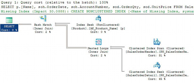
Figure 13-18. Estimated execution plan

The first thing to note is that the query was not executed. Instead, the query was passed to the optimizer inside SQL Server, and the output of the optimizer, this execution plan, was returned. There’s a lot of information to understand on this execution plan. At the top of Figure 13-18, you see the text “Query 1: Query cost (relative to the batch): 100%.” When there is more than one statement inside a query, meaning two SELECT statements, a SELECT statement and an INSERT statement, and so on, each of the individual statements within the query batch will show its estimated cost to the entire batch. In this case, there’s only one query in the batch, so it takes 100 percent of the cost. Just below that, the text of the query is listed. Next, printed in green, is Missing Index information. This will only be visible if the optimizer has identified a potential missing index. In some instances, the optimizer can recognize that an index may improve performance. When it does, it will return that information with the execution plan. Immediately below this is the graphical execution plan. A graphical plan consists of icons representing operations, or operators, within the query and arrows connecting these operations. The arrows present the flow of data from one operator to the next.

There is a lot more to be seen within the execution plan, but instead of exploring the estimated plan in detail, we’ll drill down on the actual execution plan. To enable the actual execution plan, refer to Figure 13-17. Use the icon second from the right of the figure to enable the display of actual execution plans. When you click it, nothing will happen, but it’s a switch. It will stay selected. Now execute the query. When the query completes, the result set and/or the Messages tab will be displayed as it normally would. In addition, the Execution Plan tab is visible. Click that, and you will see something similar to Figure 13-19.

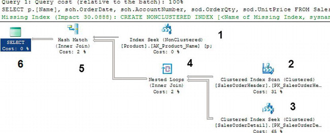
Figure 13-19. Actual execution plan, including operator order

The numbers displayed to the right of each of the operators were added and will be explained a little later. You’ll see that this actual execution plan looks more or less identical to the estimated execution plan shown in Figure 13-18. In lots of instances, the statistics on the indexes and data within the database are good enough that the estimated plan will be the same as the actual execution plan. There are, however, large differences not immediately visible, but we’ll get to those later.

Graphical execution plans show two different flows of information. They are displayed in a manner that defines the logical flow of data; there is a SELECT statement that has to pull information from a hash match operator, and so on. The physical flow of information is read from the top, right, and then down and to the left. But you have to take into account that some operations are being fed from other operators. We’ve shown the sequence that this particular execution plan is following through the numbers to the right of the operators. The first operator in sequence is the Clustered Index Scan operator at the top of the execution plan. This particular operator represents the reads necessary from the clustered index, detailed on the graphical plan, SalesOrderheader.PK_SaleOrderHeaderId. You can see a number below that: “Cost: 51%.” That number represents the optimizer’s estimates of how much this operator will cost, compared to all the other operations in the execution plan. But it’s not an actual number; it represents the number of seconds that the optimizer estimates this operation will take. These estimates are based on the statistics that the optimizer deals with and the data returned by preceding operations. When this varies, and it does frequently, these estimated costs will be wrong. However, they don’t change as the execution plan changes. The output from the Clustered Index Scan is represented by the thin little arrow pointing to operator 5. That arrow represents the rows of data coming out of the Clustered Index Scan operator. The size of the arrow is emblematic of the number of rows being moved. Because the next operation, Hash Match, relies on two feeds of data, you must resolve the feed before resolving the Hash Match operator. That’s why you then move back over to the right to find operation 2, Index Seek. The output from 2, Index Seek, feeds into 4, the Nested Loop operator. Since the Nested Loop operator has two feeds, you again must find the source of the other feed, which is 3, the other Index Seek operator. Operations 2 and 3 combine in operation 4, and then output from operation 4 combines with that of operation 1 inside operation 5. The final output goes to operation 6, the SELECT statement.

It can sound daunting and possibly even confusing to explain how the data flows from one operator to the next, but the arrows representing the rows of data should help show the order. There are more than 100 different operations and operators, so we won’t detail them here. In this instance, the operators that are taking multiple feeds represent the JOIN operations within the query that combines the data from multiple tables. A lot more information is available within the graphical execution plan. If you hover over an operator with the mouse pointer, you’ll get a tooltip displaying details about the operator. Figure 13-20 shows the tooltip for Nested Loops (Inner Join).

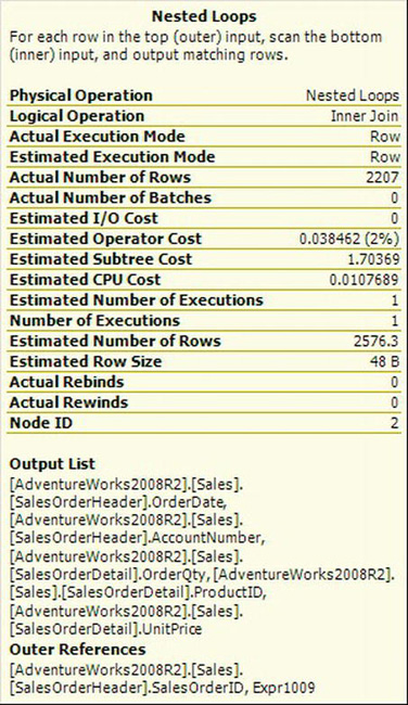
Figure 13-20. Nested Loops tooltip

The tooltip gives you a lot more information about the operator. Each of the operator tooltips is laid out in roughly the same way, although the details will vary. You can see a description at the top window that names the operator and succinctly describes what it does and how it works. Next is a listing of measurements about the operation. In these measurements, you can begin drilling down on the operators to understand what each individual operator is doing and how well it’s doing it. You can see some of the differences between the estimated and actual execution plans here. Near the top of Figure 13-20 is the measurement Actual Number of Rows and a value of 2207. Just below halfway down is the Estimated Number of Rows measurement and a value of 2576.3. This means that although there are an estimated 2576.3 rows being returned, the actual number of rows is a slightly less, at 2207. At the bottom of the tooltip are details about the operator: the output, the input, or the objects on which the operator is working. In this case, it was the output of the operator and the references used to do the loop join. When you move the mouse again, the tooltip closes.

You can also get a tooltip about the rows of information. Again, hover over the arrow instead of the operator. Figure 13-21 shows an example of the data flow tooltip.

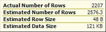
Figure 13-21. Data flow tooltip

The data flow tooltip just shows the information you see. The actual plan shows the number of rows in addition to the estimated rows available in the estimated execution plan. It’s useful to see how much data is being moved through the query.

Even more details about the operators are available. Right-click one of the operators, and select Properties from the context menu to open a properties view similar to the one shown in Figure 13-22.

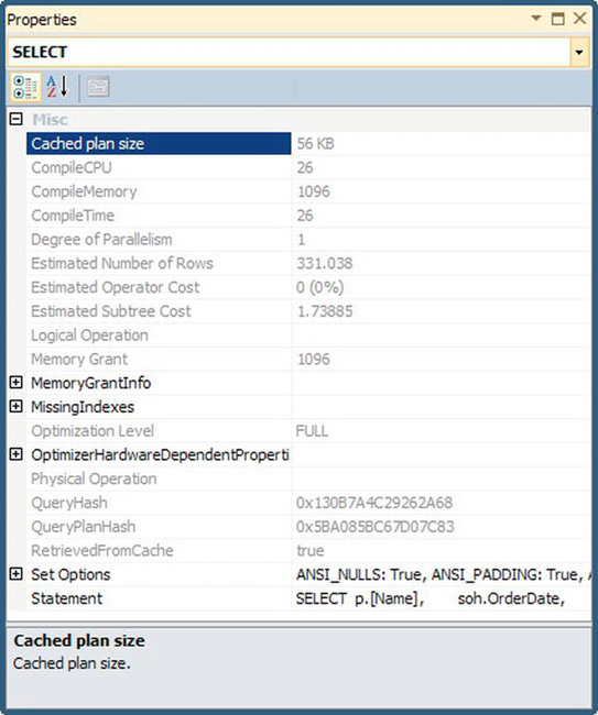
Figure 13-22. Execution plan operator properties

A lot of the information available on the tooltip is repeated here in the properties, and the Properties window has even more information available. You can open the pieces of data that have a plus sign next to them to get more information. All this is available to you so you can understand what’s happening within a query. However, getting to the information from the graphical execution plan a little bit of work. If you want to deal with nothing but raw data, you need to look at the XML execution plan.

There are a few ways to generate an XML execution plan, but since even the graphical execution plans we’ve been working with have XML behind the scenes, it’s possible to simply use a graphical plan to generate XML. Right-click inside the execution plan, and select Show Execution Plan XML. This will open a new window. Figure 13-23 shows a partial representation of an XML execution plan.

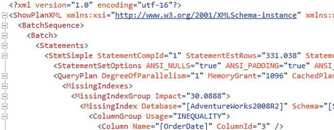
Figure 13-23. The XML execution plan

All the information available through the graphical part of the plan and from the properties of the plan is available within the XML. Unfortunately, XML is somewhat difficult to read. Primarily, you’ll use the XML plans as a means to transmit the execution plan to coworkers or support personnel. But, you can write XQuery queries against the execution plans as a way to programmatically access the information available in the execution plans; that type of query is beyond the scope of this book.

Gathering Query Information with Extended Events

Extended Events are a mechanism for gathering and viewing detailed information about the queries being executed on your system, among other things. The events provide a means to gather this information in an automated fashion so that you can use them to identify long-running or frequently called procedures. You can also gather other types of real-time information such as users logging into or out of the system, error conditions such as a deadlocks, locking information, and transactions. But the primary use is in gathering information about stored procedures as they are executed and doing this over a period of time.

Extended Event sessions are created through T-SQL commands. You can learn the T-SQL necessary to set up the commands, but you can also take advantage of the graphical user interface that was introduced in SQL Server 2012. Extended Events offer a number of methods for output of the information gathered, and we’ll focus in the two most common here. You can set up Extended Events to output to a live feed that you can watch through SSMS. You can also, in addition, set up the session to output to a file so that you can gather information over time and then report on it later at your leisure.

Extended Events operate, as we’ve already mentioned, within a construct called a session. A session is simply the definition of which events are being collected and what output you want for the events. Each event collects a default set of columns that represent information about itself. There are some columns that you can add in addition to the default columns as well as additional sets of data called actions. These can be expensive operations from a performance standpoint, and using them inappropriately can seriously impact your servers. Our suggestion is to stay away from actions until you’re 100 percent sure you’re collecting the right kind of information. The standard events and their columns will provide most of what you need anyway.

There are two graphical user interfaces that you can take advantage of for setting up Extended Event sessions. Both create the same sets of events and will start the same types of sessions. One is the standard interface used to create and edit sessions. The other is a wizard that walks you through the process of creating a session. We’ll discuss both, but we’ll spend most of our time working with the wizard. To get started with the wizard, navigate through the Object Explorer window in SSMS to the Management folder. Open that folder. Inside it is another folder called Extended Events. Expand this folder to see the folder inside labeled Sessions. Right-click the Sessions folder, and select New Session Wizard from the context menu to open the wizard shown in Figure 13-24.

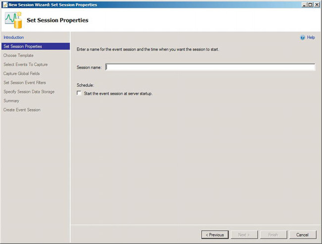
Figure 13-24. New Session Wizard for Extended Events

First, you supply a name for the session. This is a standard description and shouldn’t require much thought. We’re calling our session Gather Query Performance Metrics. You also have the option of starting a session when you start SQL Server. You can do this for gathering query metrics; just be prepared to deal with a lot of data. Once you’ve supplied a name, you can click the Next button to open the Choose Template page, shown in Figure 13-25.

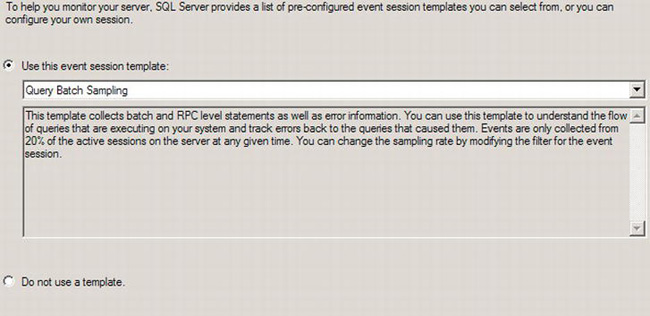
Figure 13-25. Choosing a template for the Extended Events session

On this page of the wizard, you can decide if you want to use one of the Microsoft-supplied templates or put together your own particular session. The sessions supplied by Microsoft are a great foundation to get started with. Plus, you can edit the settings that they make for you, so you’re not locked in. For a basic session that gathers query metrics, I think the Query Batch Sampling template that I have selected in Figure 13-25 is more than adequate as a starting point. You can even read about the session in the description just below the drop-down menu. Once you’ve decided whether or not you’re using a template and selected a template if you need one, you can click the Next button. You’ll see the Select Events to Capture window, shown in Figure 13-26.

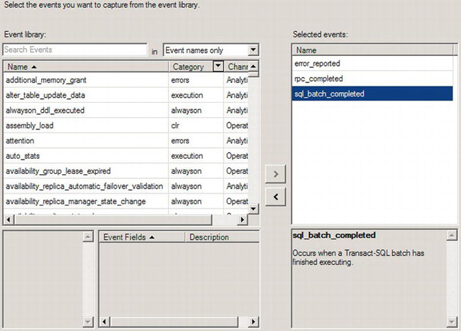
Figure 13-26. Selecting events for your Extended Events session

Three events are already selected on the right side of the screen: error_reported, rpc_completed, and sql_batch_completed. Below each of the events is a description, so you don’t have to try to decipher the names if they’re not completely clear to you. On the left side of the screen is a list of all the possible events you could capture. You can use the Search Events text box to find events and filter the information in different ways by selecting from the drop-down box next to it. If you do select additional events, you can use the little arrow buttons in the middle of the screen to move events in and out of the Selected Evens list.

The next screen is Capture Global Fields, and it contains the actions we suggested earlier that you avoid. Click Next again to open the Set Session Event Filters window, shown in Figure 13-27.

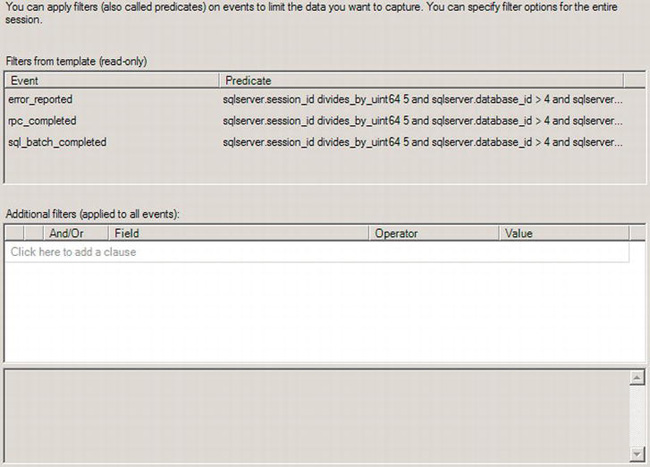
Figure 13-27. Set Session Event Filters in the Extended Events wizard

Three filters are already created for the three events in the template. You can add additional filters using the wizard page shown in Figure 13-27. You can’t edit the filters for the template within the wizard, but you can edit them once the session is created using the standard session editor. If you hover your mouse over the Predicate column for the events, you can get a look at the filters already applied, as shown in Figure 13-28.

Figure 13-28. Extended Event filter

The filter shown in Figure 13-28 tried to capture events only where the session_id is divisible by 5, therefore eliminating a substantial number of events but still capturing a representative sample. This is a valid method for gathering performance metrics on the system while keeping the overall amount of data collected low. If you’re looking for more accurate information, you’d need to edit this filter after it is created. The rest of the filter is eliminating calls to the system databases.

Clicking the Next button will open the Specify Data Storage window, visible in Figure 13-29.

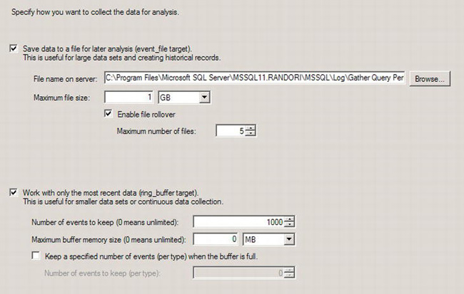
Figure 13-29. Determining where the session will output through the Specify Data Storage window

Finally, you need to determine where the information gathered during the Extended Events session will go. You can specify output to a file, to the window, or both at the same time. If you’re trying to collect performance metrics about your system, you should plan on having this information go out to a file. You can then load that information into tables at a later date for querying and aggregating the information to identify the most frequently called or most resource-intensive query.

Clicking Next will bring up a summary window where you can see all the choices that have been made while setting up this session. The back button is always available, and you can use the window choices on the left side of the screen to go back to a previous step and edit it.

When you click the Finish button, the session is created, but it is not started. This means you can decide when you want to start the session. You do get the opportunity to start it from the wizard, but having the session created, but not started, is a great way to allow you to get into the session and make any adjustments you want without having to deal with data that doesn’t meet your requirements. For the purposes of this example, we’ve started the session and launched the viewing window. The output is visible in Figure 13-30.

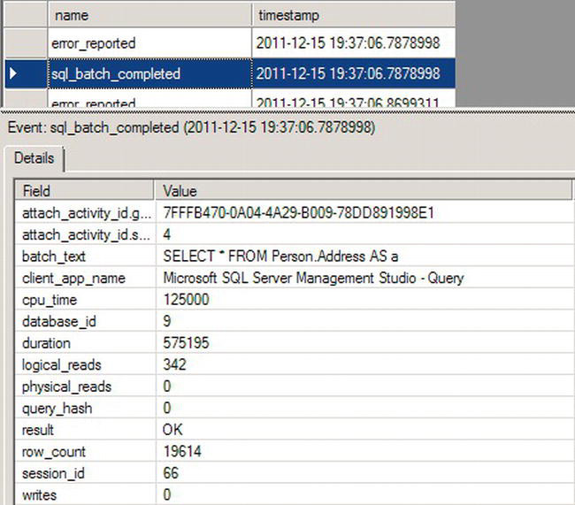
Figure 13-30. Extended Events session output

The window is divided into two parts. At the top is a series of events as they occur. Selecting a particular event will open the details in the lower window. There, you can see all the metrics that make Extended Events so incredibly useful for performance tuning. You can see the query that was called in the batch_text column. And you can see the rows returned, the number writes and reads, and the duration of the query—all necessary pieces of information when determining if the query is running fast enough or not.

Using the Database Engine Tuning Advisor

Among the principal methods that SQL Server uses to maintain and control queries are indexes and the statistics on those indexes. Taking direct control over these indexes yourself can take a lot of time and effort and require education and discovery. Fortunately, SQL Server has a tool that will help you create indexes—the Database Engine Tuning Advisor (DTA). The DTA can be run a number of different ways to help you. You can capture a trace data set and send it to the DTA for analysis. You can pass a query from the Query Editor inside Management Studio straight into the DTA for analysis. Now, with SQL Server 2012, you can use the query plans that exist in the plan cache on a server as the base data for the DTA.

To see it in action, we’ll run the DTA against the query used previously (salesquery.sql in the download):

In the query window, right-click the query text, and select Analyze Query in Database Engine Tuning Advisor from the context menu. This will open the DTA in a window that looks like Figure 13-31.

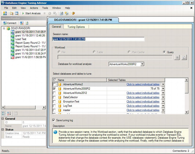
Figure 13-31. Database Engine Tuning Advisor’s General tab

Figure 13-31 shows a simple example. With more complicated examples that include data from other databases that are being run based on the workload supplied by a trace, you would have more databases selected. In this case, it’s a single query against a single database.

From here, you can move to the Tuning Options tab to adjust the possible changes being proposed by the DTA. For this example, we’ll let the default values work. On the DTA toolbar, click the Start Analysis button, and a new tab showing the progress of the analysis will open. Once the analysis completes, another new tab showing recommendations from the DTA will open. Figure 13-32 shows the recommendations for the query.

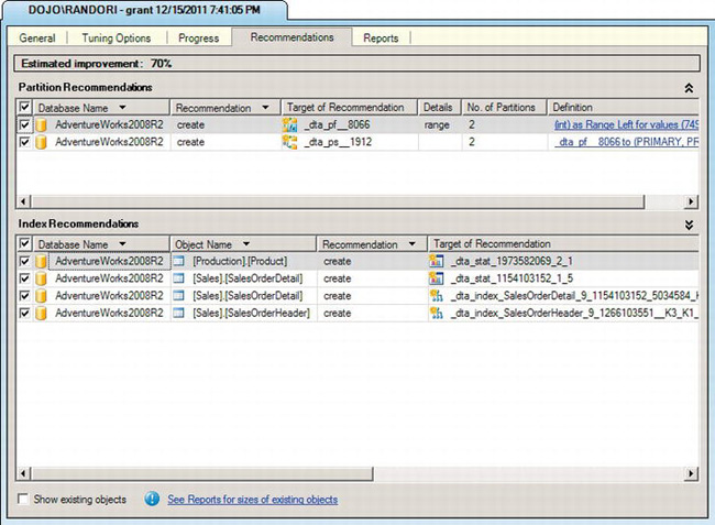
Figure 13-32. Database Engine Tuning Advisor Recommendations tab

For the query supplied, the DTA ran through the information in the query and the information in the tables, and it arrived at three indexes that it thinks will achieve a 70 percent increase in speed. You should take any and all recommendations from the DTA and test them prior to implementing them in production. It is not always right.

Managing Resources

Another way to control performance is to just prevent the processes from using as much of the CPU, memory, or disk space as possible. If any one process can’t access very much memory, more memory is available to all the other resources. If you use less space on the disks, you will have more room for growth. SQL Server 2012 supplies tools that let you manage resources. The Resource Governor lets you put hard stops on the amount of memory or CPU that requests coming in to the server can consume. Table and index compression is now built into SQL Server.

Limiting Resource Use

The Resource Governor helps you solve common problems such as queries that just run and run, consuming as many resources as they can; uneven work loads where the server is sometimes completely overwhelmed and other times practically asleep; and the ability to say that one particular process has a higher, or lower, priority than other processes. The Resource Governor will identify that a process matches a particular pattern as it arrives at the server, and it will then enforce the rules you’ve defined as appropriate for that particular pattern. Prior to setting up the Resource Governor, you will need to have a good understanding of the behavior of your application using tools already outlined such as Performance Monitor, the Data Collector, and profile traces.

When you’ve gathered at least a few days’ worth of performance data so that you know what limits you can safely impose on the system, you’ll want to configure the Resource Governor. You can control the Resource Governor through SQL Server Management Studio or T-SQL statements. T-SQL statements are going to give you more granular control and the ability to program behaviors, and they are required for some functions, but using SSMS for most functions will be easier until you have a full understanding of the concepts.

The Resource Governor is not enabled by default. To enable it, navigate to the Management folder in the Object Explorer in SSMS. Right-click the Resource Governor icon, and select Enable from the context menu. The Resource Governor is now running.

The Resource Governor works by managing the resources available in pools. A resource pool describes how much memory and CPU will be available to processes that run within that pool. To create a new pool, you first have to enable the Resource Governor by right-clicking the icon and selecting Enable Resource Governor. Next, right-click the Resource Governor icon, and choose New Resource Pool from the context menu. A window similar to Figure 13-33 will open.

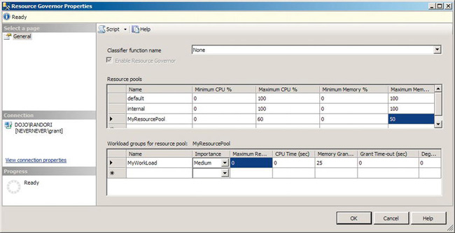
Figure 13-33. Resource Governor Properties window

We’ve created a new resource pool called MyResourcePool and placed limits on the Maximum CPU % of 60 percent and on the Maximum Memory % of 50 percent. This means that processes that run within the pool will be able to use only 60 percent of the processor power on the server and no more than 50 percent of the memory.

You define the processes that run within a pool by creating a workload. Figure 13-29 shows that we created a workload called MyWorkLoad. In the workload, you can further control the behavior of processes. These are the metrics you can control:

• Importance: This sets the priority of the particular workload within the resource pool. It doesn’t affect behavior outside that pool. This is useful for specifying which workload gets more of the resources within the pool.
• Maximum Requests: This limits the number of simultaneous requests within the pool.
• CPU Time (sec): Use this to put a limit on how long a process within the workload can wait for resources to be freed. Setting this limit gets processes out of the way if there’s a lot of stress on the server.
• Memory Grant %: This one limits how much memory can be granted from the pool to any individual process within the workload.
• Grant Time-out(sec): This is like the CPU time limit, but it limits how long the process can wait for memory.
• Degree of Parallelism: In systems with multiple processors, this limits how many processors can be used by processes within the workload.

Finally, to set up the Resource Governor to get it to recognize that processes belong to this pool and this workload, you need to define a function called a classifier. The classifier is a user-defined function that uses some sort of logic to decide whether the processes coming into the system need to be passed on to the Resource Governor. An example might be to limit the amount of resources available to queries run from Management Studio on your server. Inside the database you want to govern, you would create a function that looks something like this (governorclassifier.sql in the download):

You have to assign this to the workload only through the drop-down available in the Resource Governor Properties window, as shown in Figure 13-34. Now, when queries come in from SQL Server Management Studio, they will be limited, as defined by the workgroup and the pool, to the available resources. This will leave more resources for all other processes, thereby preventing their performance from degrading, which works out to be the same as improving it.

Leveraging Data Compression

Index and data compression are available only in the Enterprise and Developer editions of SQL Server. Data in SQL Server is stored on a construct referred to as a page. When you read data off the disk, you have to read a whole page. Frequently, especially when running queries that return large sets of data, you have to read a number of pages. Reading data from disk, as well as writing it there, are among the most expensive processes that SQL Server performs. Compression forces more data onto a page. This means that when the data is retrieved, fewer reads against the disk are necessary with more data returned. This can radically increase performance. Compression does not come without a cost, however. The process of compressing and uncompressing the data must be taken up the CPU. On systems that are already under significant stress in and around the CPU, introducing compression could be a disaster. The good news is that CPU speed keeps increasing, and it’s one of the easiest ways to increase performance. No application or code changes are required to deal with compressed data or indexes.

You can compress a table or indexes for the table separately or together. It’s worth noting that you can’t count on the compression on a table or a clustered index to automatically get transmitted to the nonclustered indexes for that table. They must be created with compression enabled individually. Compression can be implemented at the row or page level. Page compression uses row compression, and it compresses the mechanisms that describe the storage of the page. Actually, implementing either of these types of compression is simply a matter of definition when you create the table. The following script (createcompressedtable.sql in the download) shows how it works:

This will create the table dbo.MyTable with page-level compression. To create the table with row-level compression instead, just substitute ROW for PAGE in the syntax. To create an index with compression, the following syntax will work (createcompressedindex.sql in the download):

Using fewer resources for storage can and will result in performance improvements, but you will need to monitor the CPU on systems using compression.

Summary

To know how to tune your system, you first need to understand the baseline behavior that system. That’s why you use tools such as Extended Events and the data collector on systems before you’re having trouble with performance. Once you’re experiencing performance issues, you use the data collected through these tools to understand where the slowdowns are occurring. To identify what is causing the slowdowns, you would use tools like Profiler to create a trace to capture the behavior of queries and procedures. You could also write queries against dynamic management views to see the performance information stored in the system.

Once you understand what’s going wrong, you need to use execution plans to explore the behavior of the queries to find the processes that are running slowly and causing problems. With the Database Engine Tuning Advisor, you can fix some of the bad indexing on your system so that your queries will run faster. If you really need to, though, you can just limit the amount resources used by some processes through the Resource Governor. All this combines to enable you to tweak and tune the system to improve its performance and optimize its behavior.

This chapter only begins the process of explaining performance tuning. For more detail and a lot more information, check out Grant Fritchey’s SQL Server 2012 Query Performance Tuning (Apress, 2012).