
Chapter 8
![]()
Fragmentation Analysis
As explained in Chapter 4, index column values are stored in the leaf pages of an index’s B-tree structure. When you create an index (clustered or nonclustered) on a table, the cost of data retrieval is reduced by properly ordering the leaf pages of the index and the rows within the leaf pages. In an OLTP database, data changes continually, causing fragmentation of the indexes. As a result, the number of reads required to return the same number of rows increases over time.
In this chapter, I cover the following topics:
- The causes of index fragmentation, including an analysis of page splits caused by INSERT and UPDATE statements
- The overhead costs associated with fragmentation
- How to analyze the amount of fragmentation
- Techniques used to resolve fragmentation
- The significance of the fill factor in helping to control fragmentation
- How to automate the fragmentation analysis process
Causes of Fragmentation
Fragmentation occurs when data is modified in a table. When you insert or update data in a table (via INSERT or UPDATE), the table’s corresponding clustered indexes and the affected nonclustered indexes are modified. This can cause an index leaf page split if the modification to an index can’t be accommodated in the same page. A new leaf page will then be added that contains part of the original page and maintains the logical order of the rows in the index key. Although the new leaf page maintains the logical order of the data rows in the original page, this new page usually won’t be physically adjacent to the original page on the disk. Or, put a slightly different way, the logical key order of the index doesn’t match the physical order within the file.
For example, suppose an index has nine key values (or index rows) and the average size of the index rows allows a maximum of four index rows in a leaf page. As explained in Chapter 4, the 8KB leaf pages are connected to the previous and next leaf pages to maintain the logical order of the index. Figure 8-1 illustrates the layout of the leaf pages for the index.
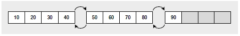
Since the index key values in the leaf pages are always sorted, a new index row with a key value of 25 has to occupy a place between the existing key values 20 and 30. Because the leaf page containing these existing index key values is full with the four index rows, the new index row will cause the corresponding leaf page to split.
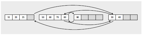
A new leaf page will be assigned to the index, and part of the first leaf page will be moved to this new leaf page so that the new index key can be inserted in the correct logical order. The links between the index pages will also be updated so that the pages are logically connected in the order of the index. As shown in Figure 8-2, the new leaf page, even though linked to the other pages in the correct logical order, can be physically out of order.
The pages are grouped together in bigger units called extents, which can contain eight pages. SQL Server uses an extent as a physical unit of allocation on the disk. Ideally, the physical order of the extents containing the leaf pages of an index should be the same as the logical order of the index. This reduces the number of switches required between extents when retrieving a range of index rows. However, page splits can physically disorder the pages within the extents, and they can also physically disorder the extents themselves. For example, suppose the first two leaf pages of the index are in extent 1, and say the third leaf page is in extent 2. If extent 2 contains free space, then the new leaf page allocated to the index because of the page split will be in extent 2, as shown in Figure 8-3.
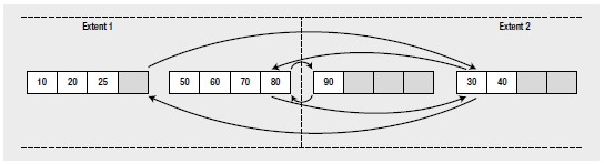
Figure 8-3. Out-of-order leaf pages distributed across extents
With the leaf pages distributed between two extents, ideally you expect to read a range of index rows with a maximum of one switch between the two extents. However, the disorganization of pages between the extents can cause more than one extent switch while retrieving a range of index rows. For example, to retrieve a range of index rows between 25 and 90, you will need three extent switches between the two extents, as follows:
- First extent switch to retrieve the key value 30 after the key value 25
- Second extent switch to retrieve the key value 50 after the key value 40
- Third extent switch to retrieve the key value 90 after the key value 80
This type of fragmentation is called external fragmentation. External fragmentation is always undesirable.
Fragmentation can also happen within an index page. If an INSERT or UPDATE operation creates a page split, then free space will be left behind in the original leaf page. Free space can also be caused by a DELETE operation. The net effect is to reduce the number of rows included in a leaf page. For example, in Figure 8-3, the page split caused by the INSERT operation has created an empty space within the first leaf page. This is known as internal fragmentation.
For a highly transactional database, it is desirable to deliberately leave some free space within your leaf pages so that you can add new rows, or change the size of existing rows, without causing a page split. In Figure 8-3, the free space within the first leaf page allows an index key value of 26 to be added to the leaf page without causing a page split.
![]() Note Note that this index fragmentation is different from disk fragmentation. The index fragmentation cannot be fixed simply by running the disk defragmentation tool, because the order of pages within a SQL Server file is understood only by SQL Server, not by the operating system.
Note Note that this index fragmentation is different from disk fragmentation. The index fragmentation cannot be fixed simply by running the disk defragmentation tool, because the order of pages within a SQL Server file is understood only by SQL Server, not by the operating system.
Heap pages can become fragmented in exactly the same way. Unfortunately, because of how heaps are stored and how any nonclustered indexes use the physical data location for retrieving data from the heap, defragmenting heaps is quite problematic. You can use the REBUILD command of ALTER TABLE to perform a heap rebuild, but understand that you will force a rebuild of any nonclustered indexes associated with that table.
SQL Server 2012 exposes the leaf pages and other data through a dynamic management view called
sys.dm_db_index_physical_stats. It stores both the index size and the fragmentation. I’ll cover it in more
detail in the next section. The DMV is much easier to work with than the old DBCC SH0WC0NTIG.
Let’s now take a look at the mechanics of fragmentation.
Page Split by an UPDATE Statement
To show what happens when a page split is caused by an UPDATE statement, I’ll use a constructed. This small test table will have a clustered index, which orders the rows within one leaf (or data) page as follows (you’ll find this code in --fragment in the code download):
IF (SELECT OBJECT_ID('Test1')
) IS NOT NULL
DROP TABLE dbo.Test1 ;
GO
CREATE TABLE dbo.Test1
(C1 INT,
C2 CHAR(999),
C3 VARCHAR(10)
)
INSERT INTO dbo.Test1
VALUES (100, 'C2', ''),
(200, 'C2', ''),
(300, 'C2', ''),
(400, 'C2', ''),
(500, 'C2', ''),
(600, 'C2', ''),
(700, 'C2', ''),
(800, 'C2', '') ;
CREATE CLUSTERED INDEX iClust
ON dbo.Test1(C1) ;
The average size of a row in the clustered index leaf page (excluding internal overhead) is not just the sum of the average size of the clustered index columns; it’s the sum of the average size of all the columns in the table, since the leaf page of the clustered index and the data page of the table are the same. Therefore, the average size of a row in the clustered index based on the foregoing sample data is as follows:
= (Average size of [C1]) + (Average size of [C2]) + (Average size of [C3]) bytes = (Size of INT) + (Size of CHAR(999)) + (Average size of data in [C3]) bytes
= 4 + 999 + 0 = 1,003 bytes
The maximum size of a row in SQL Server is 8,060 bytes. Therefore, if the internal overhead is not very high, all eight rows can be accommodated in a single 8KB page.
To determine the number of leaf pages assigned to the iClust clustered index, execute the SELECT statement against sys.dm_db_index_physical_stats:
SELECT ddips.avg_fragmentation_in_percent,
ddips.fragment_count,
ddips.page_count,
ddips.avg_page_space_used_in_percent,
ddips.record_count,
ddips.avg_record_size_in_bytes
FROM sys.dm_db_index_physical_stats(DB_ID('AdventureWorks2008R2'),
OBJECT_ID(N'dbo.Test1'), NULL,
NULL,'Sampled') AS ddips ;
You can see the results of this query in Figure 8-4.
![]()
Figure 8-4. Physical layout of index i1
From the page_count column in this output, you can see that the number of pages assigned to the clustered index is 1. You can also see the average space used, 100, in the avg_ page_space_used_in_percent column. From this you can infer that the page has no free space left to expand the content of C3, which is of type VARCHAR(10) and is currently empty.
![]() Note I’ll analyze more of the information provided by sys.dm_db_index_physical_stats in the “Analyzing the Amount of Fragmentation” section later in this chapter.
Note I’ll analyze more of the information provided by sys.dm_db_index_physical_stats in the “Analyzing the Amount of Fragmentation” section later in this chapter.
Therefore, if you attempt to expand the content of column C3 for one of the rows as follows, it should cause a page split:
UPDATE dbo.Test1
SET C3 = 'Add data'
WHERE C1 = 200 ;
Selecting the data from sys.dm_db_index_physical_stats results in the information in Figure 8-5.
![]()
Figure 8-5. i1 index after a data update
From the output in Figure 8-5, you can see that SQL Server has added a new page to the index. On a page split, SQL Server generally moves half the total number of rows in the original page to the new page. Therefore, the rows in the two pages are distributed as shown in Figure 8-6.
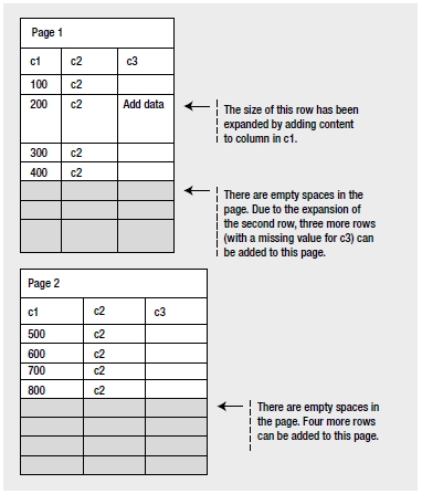
Figure 8-6. Page split caused by an UPDATE statement
From the preceding tables, you can see that the page split caused by the UPDATE statement results in an internal fragmentation of data in the leaf pages. If the new leaf page can’t be written physically next to the original leaf page, there will be external fragmentation as well. For a large table with a high amount of fragmentation, a larger number of leaf pages will be required to hold all the index rows.
Another way to look at the distribution of pages is to use some less thoroughly documented DBCC commands. First up, we can look at the pages in the table using DBCC IND:
DBCC IND(AdventureWorks2008R2,'dbo.Test1',-1)
This command lists the pages that make up a table. You get an output like Figure 8-7.
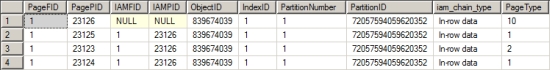
Figure 8-7. Output from DBCC IND showing two pages
If you focus on the PageType, you can see that there are now two pages of PageType = 1, which is a data page. There are other columns in the output that also show how the pages are linked together.
To show the resultant distribution of rows shown in the previous pages, you can add a trailing row to each page (--Test1_insert in the download):
INSERT INTO dbo.Test1
VALUES (410, 'C4', ''),
(900, 'C4', '') ;
These new rows are accommodated in the existing two leaf pages without causing a page split. You can confirm this by querying the other mechanism for looking at page information, DBCC PAGE. To call this, you’ll need to get the PagePID from the output of DBCC IND. This will enable you to pull back a full dump of everything on a page:
DBCC TRACEON(3604);
DBCC PAGE('AdventureWorks2008R2',1,23125,3);
The output from this is very involved to interpret, but if you scroll down to the bottom, you can see the output as shown in Figure 8-8.
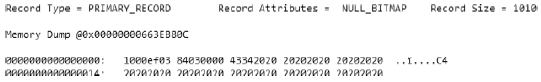
Figure 8-8. Pages after the addition of more rows
On the right side of the screen, you can see the output from the memory dump, a value, “C4”. That was added by the foregoing data. Both rows were added to one page in my tests. Getting into a full explanation of all possible permutations of these two DBCC calls is very far beyond the scope of this chapter. Know that you can determine which page data is stored on for any given table.
Page Split by an INSERT Statement
To understand how a page split can be caused by an INSERT statement, create the same test table (--fragment) as you did previously, with the eight initial rows and the clustered index. Since the single index leaf page is completely filled, any attempt to add an intermediate row as follows should cause a page split in the leaf page:
INSERT INTO Test1
VALUES (110, 'C2', '') ;
You can verify this by examining the output of sys.dm_db_index_physical_stats (Figure 8-9).
![]()
Figure 8-9. Pages after insert
As explained previously, half the rows from the original leaf page are moved to the new page. Once space
is cleared in the original leaf page, the new row is added in the appropriate order to the original leaf page.
Be aware that a row is associated with only one page; it cannot span multiple pages. Figure 8-10 shows the resultant distribution of rows in the two pages.
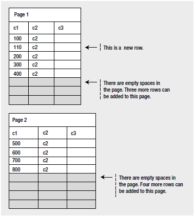
Figure 8-10. Page split caused by an INSERT statement
From the previous index pages, you can see that the page split caused by the INSERT statement spreads the rows sparsely across the leaf pages, causing internal fragmentation. It often causes external fragmentation also, since the new leaf page may not be physically adjacent to the original page. For a large table with a high amount of fragmentation, the page splits caused by the INSERT statement will require a larger number of leaf pages to accommodate all the index rows.
To demonstrate the row distribution shown in the index pages, you can run Test1_insert.sql again, adding more rows to the pages:
INSERT INTO dbo.Test1
VALUES (410, 'C4', ''),
(900, 'C4', '') ;
The result is the same as for the previous example: these new rows can be accommodated in the two existing leaf pages without causing any page split. You can validate that by calling DBCC IND and DBCC PAGE. Note that in the first page, new rows are added in between the other rows in the page. This won’t cause a page split, since free space is available in the page.
What about when you have to add rows to the trailing end of an index? In this case, even if a new page is required, it won’t split any existing page. For example, adding a new row with C1 equal to 1,300 will require a new page, but it won’t cause a page split since the row isn’t added in an intermediate position. Therefore, if new rows are added in the order of the clustered index, then the index rows will be always added at the trailing end of the index, preventing the page splits otherwise caused by the INSERT statements.
Fragmentation caused by page splits hurts data-retrieval performance, as you will see next.
Fragmentation Overhead
Both internal and external fragmentations adversely affect data-retrieval performance. External fragmentation causes a noncontiguous sequence of index pages on the disk, with new leaf pages far from the original leaf pages, and their physical ordering different from their logical ordering. Consequently, a range scan on an index will need more switches between the corresponding extents than ideally required, as explained earlier in the chapter. Also, a range scan on an index will be unable to benefit from read-ahead operations performed on the disk. If the pages are arranged contiguously, then a read-ahead operation can read pages in advance without much head movement.
For better performance, it is preferable to use sequential I/O, since this can read a whole extent (eight 8KB pages together) in a single disk I/O operation. By contrast, a noncontiguous layout of pages requires nonsequential or random I/O operations to retrieve the index pages from the disk, and a random I/O operation can read only 8KB of data in a single disk operation (this may be acceptable, however, if you are retrieving only one row). The increasing speed of hard drives, especially SSDs, has reduced the impact of this issue, but it’s still there.
In the case of internal fragmentation, rows are distributed sparsely across a large number of pages, increasing the number of disk I/O operations required to read the index pages into memory and increasing the number of logical reads required to retrieve multiple index rows from memory. As mentioned earlier, even though it increases the cost of data retrieval, a little internal fragmentation can be beneficial, because it allows you to perform INSERT and UPDATE queries without causing page splits. For queries that don’t have to traverse a series of pages to retrieve the data, fragmentation can have minimal impact.
To understand how fragmentation affects the cost of a query, create a test table with a clustered index, and insert a highly fragmented data set in the table. Since an INSERT operation in between an ordered data set can cause a page split, you can easily create the fragmented data set by adding rows in the following order (--createfragmented in the code download):
IF (SELECT OBJECT_ID('Test1’)
) IS NOT NULL
DROP TABLE dbo.Test1 ;
GO
CREATE TABLE dbo.Test1
(C1 INT,
C2 INT,
C3 INT,
c4 CHAR(2000)
) ;
CREATE CLUSTERED INDEX i1 ON dbo.Test1 (C1) ;
WITH Nums
AS (SELECT 1 AS n
UNION ALL
SELECT n + 1
FROM Nums
WHERE n < 21
)
INSERT INTO dbo.Test1
(C1, C2, C3, c4)
SELECT n,
n,
n,
'a'
FROM Nums ;
WITH Nums
AS (SELECT 1 AS n
UNION ALL
SELECT n + 1
FROM Nums
WHERE n < 21
)
INSERT INTO dbo.Test1
(C1, C2, C3, c4)
SELECT 41 - n,
n,
n,
'a'
FROM Nums;
To determine the number of logical reads required to retrieve a small result set and a large result set from this fragmented table, execute the two SELECT statements with STATISTICS IO and TIME set to ON (--fragmentstats in the download):
--Reads 6 rows
SELECT *
FROM dbo.Test1
WHERE C1 BETWEEN 21 AND 25 ;
--Reads all rows
SELECT *
FROM dbo.Test1
WHERE C1 BETWEEN 1 AND 40 ;
The number of logical reads performed by the individual queries is, respectively, as follows:
Table 'Test1'. Scan count 1, logical reads 6
CPU time = 0 ms, elapsed time = 52 ms.
Table 'Test1'. Scan count 1, logical reads 15
CPU time = 0 ms, elapsed time = 80 ms.
To evaluate how the fragmented data set affects the number of logical reads, rearrange the index leaf pages physically by rebuilding the clustered index:
ALTER INDEX i1 ON dbo.Test1 REBUILD ;
With the index leaf pages rearranged in the proper order, rerun --fragmentstats. The number of logical reads required by the preceding two SELECT statements reduces to 5 and 13, respectively:
Table 'Test1'. Scan count 1, logical reads 5
CPU time = 0 ms, elapsed time = 47 ms.
Table 'Test1'. Scan count 1, logical reads 13
CPU time = 0 ms, elapsed time = 72 ms.
Notice, though, that the execution time wasn’t radically reduced, because dropping a single page from the read just isn’t likely to increase speed much. The cost overhead because of fragmentation usually increases in line with the number of rows retrieved, because this involves reading a greater number of out-of-order pages. For point queries (queries retrieving only one row), fragmentation doesn’t usually matter, since the row is retrieved from one leaf page only, but this isn’t always the case. Because of the internal structure of the index, fragmentation may increase the cost of even a point query. For instance, the following SELECT statement (--singlestat in the download) performs two logical reads with the leaf pages rearranged properly, but it requires three logical reads on the fragmented data set. To see this in action, run --createfragmented again. Now run this query with STATISTICS IO and TIME enabled:
SELECT *
FROM dbo.Test1
WHERE C1 = 10 ;
The resulting message in the query window for this script is as follows:
Table 'Test1'. Scan count 1, logical reads 3 CPU time = 0 ms, elapsed time = 0 ms.
Once more, rebuild the index using this script:
ALTER INDEX i1 ON dbo.Test1 REBUILD;
Running the earlier SELECT statement again results in the following output:
Table 'Test1'. Scan count 1, logical reads 2
CPU time = 0 ms, elapsed time = 0 ms.
Remember that this test is on a very small scale, but the number of reads was decreased by a third. Imagine what reducing a third of the number of reads against a table with millions of rows could accomplish.
![]() Note The lesson from this section is that, for better query performance, it is important to analyze the amount of fragmentation in an index and rearrange it if required.
Note The lesson from this section is that, for better query performance, it is important to analyze the amount of fragmentation in an index and rearrange it if required.
Analyzing the Amount of Fragmentation
You can analyze the fragmentation ratio of an index by using the sys.dm_db_index_physical_ stats dynamic management function. For a table with a clustered index, the fragmentation of the clustered index is congruous with the fragmentation of the data pages, since the leaf pages of the clustered index and data pages are the same. sys.dm_db_index_physical_stats also indicates the amount of fragmentation in a heap table (or a table with no clustered index). Since a heap table doesn’t require any row ordering, the logical order of the pages isn’t relevant for the heap table.
The output of sys.dm_db_index_physical_stats shows information on the pages and extents of an index (or a table). A row is returned for each level of the B-tree in the index. A single row for each allocation unit in a heap is returned. As explained earlier, in SQL Server, eight contiguous 8KB pages are grouped together in an extent that is 64KB in size. For very small tables (much less than 64KB), the pages in an extent can belong to more than one index or table—these are called mixed extents. If there are lots of small tables in the database, mixed extents help SQL Server conserve disk space.
As a table (or an index) grows and requests more than eight pages, SQL Server creates an extent dedicated to the table (or index) and assigns the pages from this extent. Such an extent is called a uniform extent, and it serves up to eight page requests for the same table (or index). Uniform extents help SQL Server lay out the pages of a table (or an index) contiguously. They also reduce the number of page creation requests by an eighth, since a set of eight pages is created in the form of an extent. Information stored in a uniform extent can still be fragmented, but to access an allocation of pages is going to be much more efficient. If you have mixed extents, pages shared between multiple objects, and you have fragmentation within those extents, access of the information becomes even more problematic. But there is no defragmenting done on mixed extents.
To analyze the fragmentation of an index, let’s re-create the table with the fragmented data set used in the “Fragmentation Overhead” section (--createtlfragmented). You can obtain the fragmentation detail of the clustered index (Figure 8-11) by executing the query against the sys.dm_db_index_physical_stats dynamic view used earlier:
SELECT ddips.avg_fragmentation_in_percent,
ddips.fragment_count,
ddips.page_count,
ddips.avg_page_space_used_in_percent,
ddips.record_count,
ddips.avg_record_size_in_bytes
FROM sys.dm_db_index_physical_stats(DB_ID('AdventureWorks2008R2'),
OBJECT_ID(N'dbo.Test1'), NULL, NULL,
'Sampled') AS ddips ;
The dynamic management function sys.dm_db_index_physical_stats scans the pages of an index to return the data. You can control the level of the scan, which affects the speed and the accuracy of the scan. To quickly check the fragmentation of an index, use the Limited option. You can obtain an increased accuracy with only a moderate decrease in speed by using the Sample option, as in the previous example, which scans 1 percent of the pages. For the most accuracy, use the Detailed scan, which hits all the pages in an index. Just understand that the Detailed scan can have a major performance impact depending on the size of the table and index in question. If the index has fewer than 10,000 pages and you select the Sample mode, then the Detailed mode is used instead. This means that despite the choice made in the earlier query, the Detailed scan mode was used. The default mode is Limited.
By defining the different parameters, you can get fragmentation information on different sets of data. By removing the OBDECTID function in the earlier query and supplying a NULL value, the query would return information on all indexes within the database. Don’t get surprised by this and accidently run a Detailed scan on all indexes. You can also specify the index you want information on or even the partition with a partitioned index.
The output from sys.dm_db_index_physical_stats includes 21 different columns. I selected the basic set of columns used to determine the fragmentation and size of an index. This output represents the following:
- avg_fragmentation_in_percent: This number represents the logical average fragmentation for indexes and heaps as a percentage. If the table is a heap and the mode is Sampled, then this value will be NULL. If average fragmentation is less than 10 to 20 percent, fragmentation is unlikely to be an issue. If the index is between 20 and 40 percent, fragmentation might be an issue, but it can generally be resolved by defragmenting the index through an index reorganization (more information on index reorganization and index rebuild is available in the “Fragmentation Resolutions” section). Large-scale fragmentation, usually greater than 40 percent, may require an index rebuild. Your system may have different requirements than these general numbers.
- fragment_count: This number represents the number of fragments, or separated groups of pages, that make up the index. It’s a useful number to understand how the index is distributed, especially when compared to the pagecount value. fragmentcount is NULL when the sampling mode is Sampled. A large fragment count is an additional indication of storage fragmentation.
- page_count: This number is a literal count of the number of index or data pages that make up the statistic. This number is a measure of size but can also help indicate fragmentation. If you know the size of the data or index, you can calculate how many rows can fit on a page. If you then correlate this to the number of rows in the table, you should get a number close to the pagecount value. If the pagecount value is considerably higher, you may be looking at a fragmentation issue. Refer to the avg_ fragmentation_in_percent value for a precise measure.
- avg_page_space_used_in_percent: To get an idea of the amount of space allocated within the pages of the index, use this number. This value is NULL when the sampling mode is Limited.
- recordcount: Simply put, this is the number of records represented by the statistics. For indexes, this is the number of records within the current level of the B-tree as represented from the scanning mode. (Detailed scans will show all levels of the B-tree, not simply the leaf level.) For heaps, this number represents the records present, but this number may not correlate precisely to the number of rows in the table since a heap may have two records after an update and a page split.
- avg_record_size_in_bytes: This number simply represents a useful measure for the amount of data stored within the index or heap record.
Running sys.dm_db_index_physical_stats with a Detailed scan will return multiple rows for a given index. That is, multiple rows are displayed if that index spans more than one level. Multiple levels exist in an index when that index spans more than a single page. To see what this looks like and to observe some of the other columns of data present in the dynamic management function, run the query this way:
SELECT ddips.*
FROM sys.dm_db_index_physical_stats(DB_ID('AdventureWorks2008'),
OBJECT_ID(N'dbo.tlTest1'), NULL, NULL,
'Detailed') AS ddips ;
To make the data readable, I’ve broken down the resulting data table into three pieces in a single graphic;
see Figure 8-12.
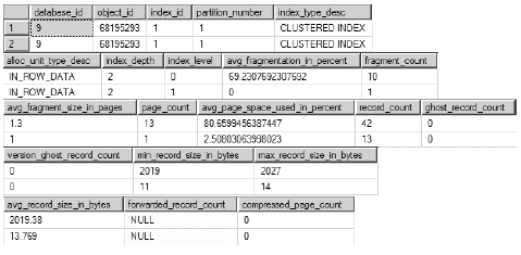
As you can see, two rows were returned, representing the leaf level of the index (index_ level = 0) and representing the first level of the B-tree (index_level = 1), which is the second row. You can see the additional information offered by sys.dm_db_index_physical_stats that can provide more detailed analysis of your indexes. For example, you can see the minimum and maximum record sizes, as well as the index depth (the number of levels in the B-tree) and how many records are on each level. A lot of this information will be less useful for basic fragmentation analysis, which is why I chose to limit the number of columns in the samples as well as use the Sampled scan mode.
Analyzing the Fragmentation of a Small Table
Don’t be overly concerned with the output of sys.dm_db_index_physical_stats for small tables. For a small table or index with fewer than eight pages, SQL Server uses mixed extents for the pages. For example, if a table (SmallTable1 or its clustered index) contains only two pages, then SQL Server allocates the two pages from a mixed extent instead of dedicating an extent to the table. The mixed extent may contain pages of other small tables/indexes also, as shown in Figure 8-13.
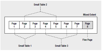
Figure 8-13. Mixed extent
The distribution of pages across multiple mixed extents may lead you to believe that there is a high amount of external fragmentation in the table or the index, when in fact this is by design in SQL Server and is therefore perfectly acceptable.
To understand how the fragmentation information of a small table or index may look, create a small table with a clustered index (--createsmalltlfragmented in the download):
IF (SELECT OBJECT_ID('dbo.Test1')
) IS NOT NULL
DROP TABLE dbo.Test1 ;
GO
CREATE TABLE dbo.Test1
(C1 INT,
C2 INT,
C3 INT,
C4 CHAR(2000)
) ;
DECLARE @n INT = 1 ;
WHILE @n <= 28
BEGIN
INSERT INTO dbo.Test1
VALUES (@n, @n, @n, 'a') ;
SET @n = @n + 1 ;
END
CREATE CLUSTERED INDEX FirstIndex ON dbo.Test1(C1) ;
In the preceding table, with each INT taking 4 bytes, the average row size is 2,012 (=4 + 4 + 4 + 2,000) bytes. Therefore, a default 8KB page can contain up to four rows. After all 28 rows are added to the table, a clustered index is created to physically arrange the rows and reduce fragmentation to a minimum. With the minimum internal fragmentation, seven (= 28 / 4) pages are required for the clustered index (or the base table). Since the number of pages is not more than eight, SQL Server uses pages from mixed extents for the clustered index (or the base table). If the mixed extents used for the clustered index are not side by side, then the output of sys.dm_db_index_physical_stats may express a high amount of external fragmentation. But as a SQL user, you can’t reduce the resultant external fragmentation. Figure 8-14 shows the output of sys.dm_db_index_physical_stats.
![]()
Figure 8-14. Fragmentation of a small clustered index
From the output of sys.dm_db_index_physical_stats, you can analyze the fragmentation of the small clustered index (or the table) as follows:
- avgfragmentationinpercent: Although this index may cross to multiple extents, the fragmentation shown here is not an indication of external fragmentation because this index is being stored on mixed extents.
- avgpagespaceusedinpercent: This shows that all or most of the data is stored well within the seven pages displayed in the pagecount field. This eliminates the possibility of logical fragmentation.
- fragmentcount: This shows that the data is fragmented and stored on more than one extent, but since it’s less than eight pages long, SQL Server doesn’t have much choice about where it stores the data.
In spite of the preceding misleading values, a small table (or index) with fewer than eight pages is simply unlikely to benefit from efforts to remove the fragmentation because it will be stored on mixed extents.
Once you determine that fragmentation in an index (or a table) needs to be dealt with, you need to decide which defragmentation technique to use. The factors affecting this decision, and the different techniques, are explained in the following section.
Fragmentation Resolutions
You can resolve fragmentation in an index by rearranging the index rows and pages so that their physical and logical orders match. To reduce external fragmentation, you can physically reorder the leaf pages of the index to follow the logical order of the index. You achieve this through the following techniques:
- Dropping and re-creating the index
- Re-creating the index with the DROP_EXISTING clause
- Executing the ALTER INDEX REBUILD statement on the index
- Executing the ALTER INDEX REORGANIZE statement on the index
Dropping and Re-creating the Index
One of the apparently easiest ways to remove fragmentation in an index is to drop the index and then re-create it. Dropping and re-creating the index reduces fragmentation the most, since it allows SQL Server to use completely new pages for the index and populate them appropriately with the existing data. This avoids both internal and external fragmentation. Unfortunately, this method has a large number of shortcomings:
- Blocking: This technique of defragmentation adds a high amount of overhead on the system, and it causes blocking. Dropping and re-creating the index blocks all other requests on the table (or on any other index on the table). It can also be blocked by other requests against the table.
- Missing index: With the index dropped, and possibly being blocked and waiting to be re-created, queries against the table will not have the index available for use. This can lead to the poor performance that the index was intended to remedy.
- Nonclustered indexes: If the index being dropped is a clustered index, then all the nonclustered indexes on the table have to be rebuilt after the cluster is dropped. They then have to be rebuilt again after the cluster is re-created. This leads to further blocking and other problems such as statement recompiles (covered in detail in Chapter 10).
- Unique constraints: Indexes that are used to define a primary key or a unique constraint cannot be removed using the DROP INDEX statement. Also, both unique constraints and primary keys can be referred to by foreign key constraints. Prior to dropping the primary key, all foreign keys that reference the primary key would have to be removed first. Although this is possible, this is a risky and time-consuming method for defragmenting an index.
It is possible to use the ONLINE option for dropping a clustered index, which means the index is still readable while it is being dropped, but that saves you only from the foregoing blocking issue. For all these reasons, dropping and re-creating the index is not a recommended technique for a production database, especially at anything outside off-peak times.
Re-creating the Index with the DROP_EXISTING Clause
To avoid the overhead of rebuilding the nonclustered indexes twice while rebuilding a clustered index, use the DROPEXISTING clause of the CREATE INDEX statement. This re-creates the clustered index in one atomic step, avoiding re-creating the nonclustered indexes since the clustered index key values used by the row locators remain the same. To rebuild a clustered key in one atomic step using the DROPEXISTING clause, execute the CREATE INDEX statement as follows:
CREATE UNIQUE CLUSTERED INDEX FirstIndex
ON dbo.Test1(C1)
WITH (DROP_EXISTING = ON) ;
You can use the DROP_EXISTING clause for both clustered and nonclustered indexes, and even to convert a nonclustered index to a clustered index. However, you can’t use it to convert a clustered index to a nonclustered index.
The drawbacks of this defragmentation technique are as follows:
- Blocking: Similar to the DROP and CREATE methods, this technique also causes and faces blocking from other queries accessing the table (or any index on the table).
- Index with constraints: Unlike the first method, the CREATE INDEX statement with DROP_EXISTING can be used to re-create indexes with constraints. If the constraint is a primary key or the unique constraint is associated with a foreign key, then failing to include the UNIQUE keyword in the CREATE statement will result in an error like this:
![]() Msg 1907, Level 16, State 1, Line 1 Cannot recreate index ‘PK_Name’. The new index definition does not match the constraint being enforced by the existing index.
Msg 1907, Level 16, State 1, Line 1 Cannot recreate index ‘PK_Name’. The new index definition does not match the constraint being enforced by the existing index.
- Table with multiple fragmented indexes: As table data fragments, the indexes often become fragmented as well. If this defragmentation technique is used, then all the indexes on the table have to be identified and rebuilt individually.
You can avoid the last two limitations associated with this technique by using ALTER INDEX REBUILD, as explained next.
Executing the ALTER INDEX REBUILD Statement
ALTER INDEX REBUILD rebuilds an index in one atomic step, just like CREATE INDEX with the DROP_EXISTING clause. Since ALTER INDEX REBUILD also rebuilds the index physically, it allows SQL Server to assign fresh pages to reduce both internal and external fragmentation to a minimum. But unlike CREATE INDEX with the DROP_EXISTING clause, it allows an index (supporting either the PRIMARY KEY or UNIQUE constraint) to be rebuilt dynamically without dropping and re-creating the constraints.
To understand the use of ALTER INDEX REBUILD to defragment an index, consider the fragmented table used in the “Fragmentation Overhead” and “Analyzing the Amount of Fragmentation” sections (--createfragmented). This table is repeated here:
IF (SELECT OBJECT_ID('Test1')
) IS NOT NULL
DROP TABLE dbo.Test1 ;
GO
CREATE TABLE dbo.Test1
(C1 INT,
C2 INT,
C3 INT,
c4 CHAR(2000)
) ;
CREATE CLUSTERED INDEX i1 ON dbo.Test1 (C1) ;
WITH Nums
AS (SELECT 1 AS n
UNION ALL
SELECT n + 1
FROM Nums
WHERE n < 21
)
INSERT INTO dbo.Test1
(C1, C2, C3, c4)
SELECT n,
n,
n,
'a'
FROM Nums ;
WITH Nums
AS (SELECT 1 AS n
UNION ALL
SELECT n + 1
FROM Nums
WHERE n < 21
)
INSERT INTO dbo.Test1
(C1, C2, C3, c4)
SELECT 41 - n,
n,
n,
'a'
FROM Nums;
If you take a look at the current fragmentation, you can see that it is both internally and externally fragmented (Figure 8-15).
![]()
Figure 8-15. Internal and external fragmentation
You can defragment the clustered index (or the table) by using the ALTER INDEX REBUILD statement:
ALTER INDEX i1 ON dbo.Test1 REBUILD;
Figure 8-16 shows the resultant output of the standard SELECT statement against sys. dm_db_index_physical_stats.
![]()
Figure 8-16. Fragmentation resolved by ALTER INDEX REBUILD
Compare the preceding results of the query in Figure 8-16 with the earlier results in Figure 8-15. You can see that both internal and external fragmentation have been reduced efficiently. Here’s an analysis of the output:
- Internal fragmentation: The table has 42 rows with an average row size (2,019.38 bytes) that allows a maximum of four rows per page. If the rows are highly defragmented to reduce the internal fragmentation to a minimum, then there should be 11 data pages in the table (or leaf pages in the clustered index). You can observe the following in the preceding output:
- Number of leaf (or data) pages: pagecount = 11
- Amount of information in a page: avg_page_space_used_in_percent = 95.33 percent
- External fragmentation: A minimum of two extents is required to hold the 11 pages. For a minimum of external fragmentation, there should not be any gap between the two extents, and all pages should be physically arranged in the logical order of the index. The preceding output illustrates the number of out-of-order pages = avg_ fragmentation_in_percent = 27.27 percent. Although this may not be a perfect level of fragmentation, being greater than 20 percent, this is adequate considering the size of the index. With fewer extents, aligned with each other, access will be faster.
Rebuilding an index in SQL Server 2005 and greater will also compact the large object (LOB) pages. You can choose not to by setting a value LOB_COMPACTION = OFF.
When you use the PAD_INDEX setting while creating an index, it determines how much free space to leave on the index intermediate pages, which can help you deal with page splits. This is taken into account during the index rebuild, and the new pages will be set back to the original values you determined at the index creation unless you specify otherwise.
If you don’t specify otherwise, the default behavior is to defragment all indexes across all partitions. If you want to control the process, you just need to specify which partition you want to rebuild when.
As shown previously, the ALTER INDEX REBUILD technique effectively reduces fragmentation. You can also use it to rebuild all the indexes of a table in one statement:
ALTER INDEX ALL ON dbo.Test1 REBUILD;
Although this is the most effective defragmentation technique, it does have some overhead and limitations:
- Blocking: Similar to the previous two index-rebuilding techniques, ALTER INDEX REBUILD introduces blocking in the system. It blocks all other queries trying to access the table
(or any index on the table). It can also be blocked by those queries. - Transaction rollback: Since ALTER INDEX REBUILD is fully atomic in action, if it is stopped before completion, then all the defragmentation actions performed up to that time are lost. You can run ALTER INDEX REBUILD using the ONLINE keyword, which will reduce the locking mechanisms, but it will increase the time involved in rebuilding the index.
Executing the ALTER INDEX REORGANIZE Statement
ALTER INDEX REORGANIZE reduces the fragmentation of an index without rebuilding the index. It reduces external fragmentation by rearranging the existing leaf pages of the index in the logical order of the index key. It compacts the rows within the pages, reducing internal fragmentation, and discards the resultant empty pages. This technique doesn’t use any new pages for defragmentation.
To avoid the blocking overhead associated with ALTER INDEX REBUILD, this technique uses a nonatomic online approach. As it proceeds through its steps, it requests a small number of locks for a short period. Once each step is done, it releases the locks and proceeds to the next step. While trying to access a page, if it finds that the page is being used, it skips that page and never returns to the page again. This allows other queries to run on the table along with the ALTER INDEX REORGANIZE operation. Also, if this operation is stopped intermediately, then all the defragmentation steps performed up to then are preserved.
Since ALTER INDEX REORGANIZE doesn’t use any new pages to reorder the index and it skips the locked pages, the amount of defragmentation provided by this approach is usually less than that of ALTER INDEX REBUILD. To observe the relative effectiveness of ALTER INDEX REORGANIZE compared to ALTER INDEX REBUILD, rebuild the test table (--createfragmented) used in the previous section on ALTER INDEX REBUILD.
Now, to reduce the fragmentation of the clustered index, use ALTER INDEX REORGANIZE as follows:
ALTER INDEX i1 ON dbo.Test1 REORGANIZE;
Figure 8-17 shows the resultant output from sys.dm_db_index_physical_stats.
![]()
Figure 8-17. Results of ALTER INDEX REORGANIZE
From the output, you can see that ALTER INDEX REORGANIZE doesn’t reduce fragmentation as effectively as ALTER INDEX REBUILD, as shown in the previous section. For a highly fragmented index, the ALTER INDEX REORGANIZE operation can take much longer than rebuilding the index. Also, if an index spans multiple files, ALTER INDEX REORGANIZE doesn’t migrate pages between the files. However, the main benefit of using ALTER INDEX REORGANIZE is that it allows other queries to access the table (or the indexes) simultaneously.
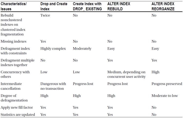
Table 8-1 summarizes the characteristics of these four defragmentation techniques.
Table 8-1. Characteristics of Four Defragmentation Techniques
You can also reduce internal fragmentation by compressing more rows within a page, reducing free spaces within the pages. The maximum amount of compression that can be done within the leaf pages of an index is controlled by the fill factor, as you will see next.
When dealing with very large databases and the indexes associated, it may become necessary to split the tables and the indexes up across disks using partitioning. Indexes on partitions can also become fragmented as the data within the partition changes. When dealing with a portioned index, you will need to determine whether you want to either REORGANIZE or REBUILD one, some, or all partitions as part of the ALTER INDEX command. Partitioned indexes cannot be rebuilt online. Keep in mind that doing anything that affects all partitions is likely to be a very costly operation.
If compression is specified on an index, even on a partitioned index, you must be sure to set the compression while performing the ALTER INDEX operation to what it was before; if you don’t, it will be lost, and you’ll have to rebuild the index again. This is especially important for nonclustered indexes, which will not inherit the compression setting from the table.
Significance of the Fill Factor
The internal fragmentation of an index is reduced by getting more rows per leaf page in an index. Getting more rows within a leaf page reduces the total number of pages required for the index and in turn decreases disk I/O and the logical reads required to retrieve a range of index rows. On the other hand, if the index key values are highly transactional, then having fully used index pages will cause page splits. Therefore, for a transactional table, a good balance between maximizing the number of rows in a page and avoiding page splits is required.
SQL Server allows you to control the amount of free space within the leaf pages of the index by using the fill factor. If you know that there will be enough INSERT queries on the table or UPDATE queries on the index key columns, then you can pre-add free space to the index leaf page using the fill factor to minimize page splits. If the table is read-only, you can create the index with a high fill factor to reduce the number of index pages.
The default fill factor is 0, which means the leaf pages are packed to 100 percent, although some free space is left in the branch nodes of the B-tree structure. The fill factor for an index is applied only when the index is created. As keys are inserted and updated, the density of rows in the index eventually stabilizes within a narrow range. As you saw in the previous chapter’s sections on page splits caused by UPDATE and INSERT, when a page split occurs, generally half the original page is moved to a new page, which happens irrespective of the fill factor used during the index creation.
To understand the significance of the fill factor, let’s use a small test table (--filltest in the download) with 24 rows:
IF (SELECT OBJECT_ID('dbo.Test1')
) IS NOT NULL
DROP TABLE dbo.Test1;
GO
CREATE TABLE dbo.Test1 (C1 INT, C2 CHAR(999)) ;
WITH Nums
AS (SELECT 1 AS n
UNION ALL
SELECT n + 1
FROM Nums
WHERE n < 24
)
INSERT INTO dbo.Test1
(C1, C2)
SELECT n * 100,
'a'
FROM Nums ;
Increase the maximum number of rows in the leaf (or data) page by creating a clustered index with the default fill factor:
CREATE CLUSTERED INDEX FillIndex ON Test1(C1);
Since the average row size is 1,010 bytes, a clustered index leaf page (or table data page) can contain a maximum of eight rows. Therefore, at least three leaf pages are required for the 24 rows. You can confirm this in the sys.dm_db_index_physical_stats output shown in Figure 8-18.
![]()
Figure 8-18. Fill factor set to default value of 0
Note that avg_page_space_used_in_percent is 100 percent, since the default fill factor allows the maximum number of rows to be compressed in a page. Since a page cannot contain a part row to fill the page fully,
avg_page_space_used_in_percent will be often a little less than 100 percent, even with the default fill factor.
To prevent page splits caused by INSERT and UPDATE operations, create some free space within the leaf (or data) pages by re-creating the clustered index with a fill factor as follows:
ALTER INDEX FillIndex ON dbo.Test1 REBUILD
WITH (FILLFACTOR= 75) ;
Because each page has a total space for eight rows, a fill factor of 75 percent will allow six rows per page. Thus, for 24 rows, the number of leaf pages should increase to four, as in the sys.dm_db_index_physical_stats output shown in Figure 8-19.
![]()
Figure 8-19. Fill factor set to 75
Note that avg_page_space_used_in_percent is about 75 percent, as set by the fill factor. This allows two more rows to be inserted in each page without causing a page split. You can confirm this by adding two rows to the first set of six rows (C1 = 100 - 600, contained in the first page):
INSERT INTO dbo.Test1
VALUES (110, 'a'), --25th row
(120, 'a') ; --26th row
Figure 8-20 shows the current fragmentation.
![]()
Figure 8-20. Fragmentation after new records
From the output, you can see that the addition of the two rows has not added any pages to the index. Accordingly, avg_page_space_used_in_percent increased from 74.99 percent to 81.25 percent. With the addition of two rows to the set of the first six rows, the first page should be completely full (eight rows). Any further addition of rows within the range of the first eight rows should cause a page split and thereby increase the number of index pages to five:
INSERT INTO dbo.Test1
VALUES (130, 'a') ; --27th row
Now sys.dm_db_index_physical_stats displays the difference in Figure 8-21.
![]()
Figure 8-21. Number of pages goes up
Note that even though the fill factor for the index is 75 percent, Avg. Page Density (full) has decreased to 67.49 percent, which can be computed as follows:
Avg. Page Density (full)
= Average rows per page / Maximum rows per page
= (27 / 5) / 8
= 67.5%
From the preceding example, you can see that the fill factor is applied when the index is created. But later, as the data is modified, it has no significance. Irrespective of the fill factor, whenever a page splits, the rows of the original page are distributed between two pages, and avg_page_space_used_in_percent settles accordingly. Therefore, if you use a nondefault fill factor, you should ensure that the fill factor is reapplied regularly to maintain its effect.
You can reapply a fill factor by re-creating the index or by using ALTER INDEX REORGANIZE or ALTER INDEX REBUILD, as was shown. ALTER INDEX REORGANIZE takes the fill factor specified during the index creation into account. ALTER INDEX REBUILD also takes the original fill factor into account, but it allows a new fill factor to be specified, if required.
Without periodic maintenance of the fill factor, for both default and nondefault fill factor settings, avg_page_space_used_in_percent for an index (or a table) eventually settles within a narrow range. Therefore, in most cases, without manual maintenance of the fill factor, the default fill factor is generally good enough.
You should also consider one final aspect when deciding upon the fill factor. Even for a heavy OLTP application, the number of database reads typically outnumbers writes by a factor of 5 to 10. Specifying a fill factor other than the default can degrade read performance by an amount inversely proportional to the fill factor setting, since it spreads keys over a wider area. Before setting the fill factor at a database-wide level, use Performance Monitor to compare the SOL Server:Buffer Manager:Page reads/sec counter to the SOL Server:Buffer Manager:Page writes/sec counter, and use the fill factor option only if writes are a substantial fraction of reads (greater than 30 percent).
Automatic Maintenance
In a database with a great deal of transactions, tables and indexes become fragmented over time. Thus, to improve performance, you should check the fragmentation of the tables and indexes regularly, and you should defragment the ones with a high amount of fragmentation. You can do this analysis for a database by following these steps:
1. Identify all user tables in the current database to analyze fragmentation.
2. Determine fragmentation of every user table and index.
3. Determine user tables and indexes that require defragmentation by taking into account the following considerations:
- high level of fragmentation where avg_fragmentation_in_percent is greater than
20 percent - Not a very small table/index—that is, pagecount is greater than 8
4. Defragment tables and indexes with high fragmentation.
A sample SQL stored procedure (IndexDefrag.sql in the download) is included here for easy reference. This script will perform the basic actions, and I include it here for educational purposes. But for a fully functional script that includes a large degree of capability, I strongly recommend using the script from Michelle Ufford located here: http://sqlfool.com/wp-content/uploads/2011/06/dba_indexDefrag_sp_v41.txt
My script performs the following actions:
- Walks all databases on the system and identifies indexes on user tables in each database that meets the fragmentation criteria and saves them in a temporary table
- Based on the level of fragmentation, reorganizes lightly fragmented indexes and rebuilds those that are highly fragmented
Here’s how to analyze and resolve database fragmentation (store this where appropriate on your system; we have a designated database for enterprise-level scripts):
CREATE PROCEDURE IndexDefrag
AS
DECLARE @DBName NVARCHAR(255),
@TableName NVARCHAR(255),
@SchemaName NVARCHAR(255),
@IndexName NVARCHAR(255),
@PctFrag DECIMAL,
@Defrag NVARCHAR(MAX)
IF EXISTS ( SELECT *
FROM sys.objects
WHERE object_id = OBJECT_ID(N'#Frag') )
DROP TABLE #Frag ;
CREATE TABLE #Frag
(DBName NVARCHAR(255),
TableName NVARCHAR(255),
SchemaName NVARCHAR(255),
IndexName NVARCHAR(255),
AvgFragment DECIMAL
)
EXEC sys.sp_MSforeachdb
'INSERT INTO #Frag ( DBName, TableName, SchemaName, IndexName, AvgFragment ) SELECT ''?'' AS DBName ,t.Name AS TableName ,sc.Name AS SchemaName ,i.name AS IndexName ,s.avg_fragmentation_in_percent FROM ?.sys.dm_db_index_physical_stats(DB_ID(''?''), NULL, NULL,
NULL, ''Sampled'') AS s JOIN ?.sys.indexes i ON s.Object_Id = i.Object_id
AND s.Index_id = i.Index_id JOIN ?.sys.tables t ON i.Object_id = t.Object_Id JOIN ?.sys.schemas sc ON t.schema_id = sc.SCHEMA_ID
WHERE s.avg_fragmentation_in_percent > 20
AND t.TYPE = ''U''
AND s.page_count > 8
ORDER BY TableName,IndexName' ;
DECLARE cList CURSOR
FOR
SELECT *
FROM #Frag
OPEN cList ;
FETCH NEXT FROM cList
INTO @DBName, @TableName, @SchemaName, @IndexName, @PctFrag ;
WHILE @@FETCH_STATUS = 0
BEGIN
IF @PctFrag BETWEEN 20.0 AND 40.0
BEGIN
SET @Defrag = N'ALTER INDEX ' + @IndexName + ' ON ' + @DBName
+ '.' + @SchemaName + '.' + @TableName + ' REORGANIZE' ;
EXEC sp_executesql
@Defrag ;
PRINT 'Reorganize index: ' + @DBName + '.' + @SchemaName + '.'
+ @TableName + '.' + @IndexName ;
END
ELSE
IF @PctFrag > 40.0
BEGIN
SET @Defrag = N'ALTER INDEX ' + @IndexName + ' ON '
+ @DBName + '.' + @SchemaName + '.' + @TableName
+ ' REBUILD' ;
EXEC sp_executesql
@Defrag ;
PRINT 'Rebuild index: ' + @DBName + '.' + @SchemaName
+ '.' + @TableName + '.' + @IndexName ;
END
FETCH NEXT FROM cList
INTO @DBName, @TableName, @SchemaName, @IndexName, @PctFrag ;
END
CLOSE cList ;
DEALLOCATE cList ;
DROP TABLE #Frag ;
GO
To automate the fragmentation analysis process, you can create a SQL Server job from SQL Server Enterprise Manager by following these simple steps:
1. Open Management Studio, right-click the SQL Server Agent icon, and select New ä Job.
2. On the General page of the New Job dialog box, enter the job name and other details, as shown in Figure 8-22.
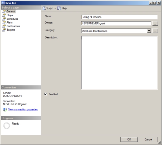
Figure 8-22. Entering the job name and details
3. On the Steps page of the New Job dialog box, click New, and enter the SQL command for the user database, as shown in Figure 8-23.
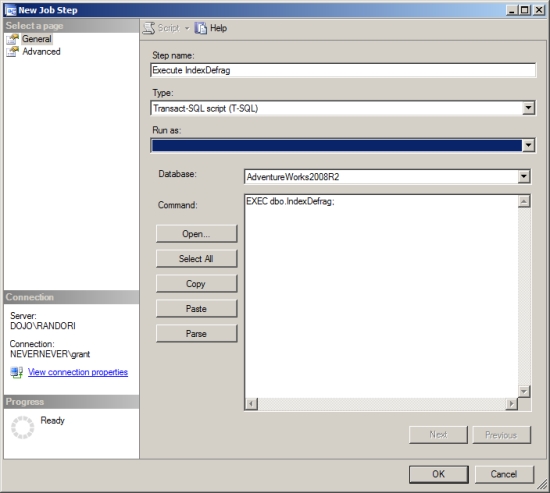
Figure 8-23. Entering the SQL command for the user database
4. On the Advanced page of the New Job Step dialog box, enter an output file name to report the fragmentation analysis outcome, as shown in Figure 8-24.
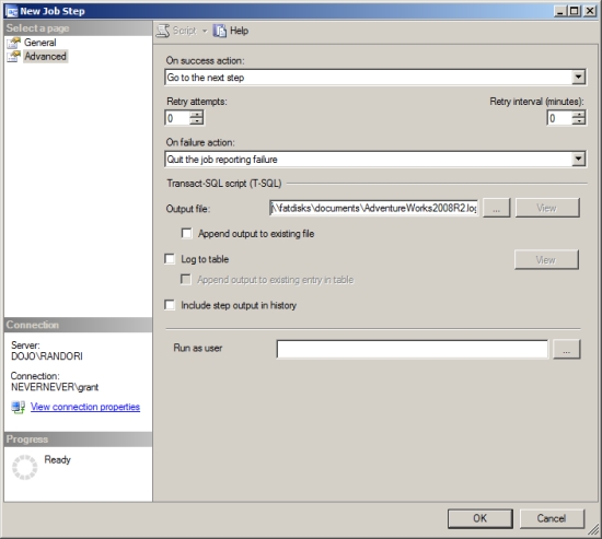
Figure 8-24. Entering an output file name
5. Return to the New Job dialog box by clicking OK.
6. On the Schedules page of the New Job dialog box, click New Schedule, and enter an appropriate schedule to run the SQL Server job, as shown in Figure 8-25.Schedule this stored procedure to execute during nonpeak hours. To be certain about the usage pattern of your database, log the SQLServer:SOL StatisticsBatch Requests/ sec performance counter for a complete day. It will show you the fluctuation in load on the database. (I explain this performance counter in detail in Chapter 2.)
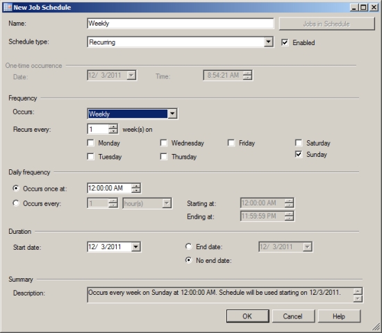
Figure 8-25. Entering a job schedule
7. Return to the New Job dialog box by clicking the OK button.
8. Once you’ve entered all the information, click OK in the New Job dialog box to create the SQL Server job. A SQL Server job is created that schedules the spIndexDefrag stored procedure to run at a regular (weekly) time interval.
9. Ensure that SQL Server Agent is running so that the SQL Server job will run automatically according to the set schedule.
The SQL job will automatically analyze and defragment the fragmentation of each database every Sunday at 1 a.m. Figure 8-26 shows the corresponding output of the FragmentationOutput.txt file.
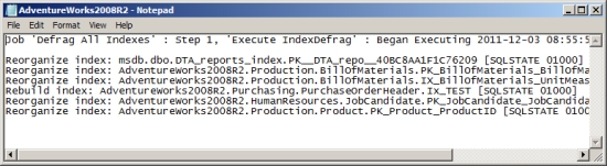
Figure 8-26. FragmentationOutput.txt file output
The output shows that the job analyzed the fragmentation of the database and identified a series of indexes for defragmentation, specifically for reorganization. Subsequently, it defragments the index. The stored procedure defragmented only the database object that was highly fragmented. Thus, the next run of the SQL job generally won’t identify these same indexes for defragmentation.
Summary
As you learned in this chapter, in a highly transactional database page splits caused by INSERT and UPDATE statements fragment the tables and indexes, increasing the cost of data retrieval. You can avoid these page splits by maintaining free spaces within the pages using the fill factor. Since the fill factor is applied only during index creation, you should reapply it at regular intervals to maintain its effectiveness. You can determine the amount of fragmentation in an index (or a table) using sys.dm_db_index_physical_stats. Upon determining a high amount of fragmentation, you can use either ALTER INDEX REBUILD or ALTER INDEX REORGANIZE, depending on the required amount of defragmentation and database concurrency.
Defragmentation rearranges the data so that its physical order on the disk matches its logical order in the table/index, thus improving the performance of queries. However, unless the optimizer decides upon an effective execution plan for the query, query performance even after defragmentation can remain poor. Therefore, it is important to have the optimizer use efficient techniques to generate cost-effective execution plans.
In the next chapter, I explain execution plan generation and the techniques the optimizer uses to decide upon an effective execution plan.