
![]()
At the heart of some applications lie specialized algorithms designed for a specific domain and based on assumptions that do not hold universally. Other applications rely on well-tested algorithms that fit many domains and have been relevant for decades in the entire field of computer software. We believe that every software developer can benefit and obtain insight from some of the crown jewels of algorithms research, as well as the algorithm categories on which software frameworks are based. Although some parts of this chapter might be somewhat difficult if you do not have a strong mathematical background, they are well worth the effort.
This chapter gently brushes against some of the pillars of computer science and reviews several examples of immortal algorithms and their complexity analysis. Supplied with these examples, you should feel more comfortable using existing algorithms, adapting them to your needs, and inventing your own.
![]() Note This is not a textbook on algorithms research, nor an introductory text into the most important algorithms in modern computer science. This chapter is deliberately short to make it explicitly clear that you cannot learn from it all you need to know. We have not delved into formal definitions in any detail. For example, our treatment of Turing machines and languages is not at all rigorous. For a textbook introduction to algorithms, consider Cormen, Leiserson, Rivest, and Stein’s “Introduction to Algorithms” (MIT Press, 2001) and Dasgupta, Papadimitriou, and Vazirani’s “Algorithms” (soon to appear, currently available online as a draft).
Note This is not a textbook on algorithms research, nor an introductory text into the most important algorithms in modern computer science. This chapter is deliberately short to make it explicitly clear that you cannot learn from it all you need to know. We have not delved into formal definitions in any detail. For example, our treatment of Turing machines and languages is not at all rigorous. For a textbook introduction to algorithms, consider Cormen, Leiserson, Rivest, and Stein’s “Introduction to Algorithms” (MIT Press, 2001) and Dasgupta, Papadimitriou, and Vazirani’s “Algorithms” (soon to appear, currently available online as a draft).
Chapter 5 had the chance to briefly mention the complexity of some operations on the .NET Framework’s collections and some collections of our own implementation. This section defines more accurately what Big-Oh complexity means and reviews the main complexity classes known in computability and complexity theory.
When we discussed the complexity of a lookup operation on a List<T> in Chapter 5, we said it had runtime complexity O(n). What we meant to say informally is that, when you have a list of 1,000 items and are trying to find in it another item, then the worst-case running time of that operation is 1,000 iterations through the list—namely, if the item is not already in the list. Thus, we try to estimate the order of magnitude of the running time’s growth as the inputs become larger. When specified formally, however, the Big-Oh notation might appear slightly confusing:
Suppose that the function T(A;n) returns the number of computation steps required to execute the algorithm A on an input size of n elements, and let f(n) be a monotonic function from positive integers to positive integers. Then, T(A;n) is O(f(n)), if there exists a constant c such that for all n, T(A;n) ≤ cf(n).
In a nutshell, we can say that an algorithm’s runtime complexity is O(f(n)), if f(n) is an upper bound on the actual number of steps it takes to execute the algorithm on an input of size n. The bound does not have to be tight; for example, we can also say that List<T> lookup has runtime complexity O(n4). However, using such a loose upper bound is not helpful, because it fails to capture the fact that it is realistic to search a List<T> for an element even if it has 1,000,000 elements in it. If List<T> lookup had tight runtime complexity O(n4), it would be highly inefficient to perform lookups even on lists with several thousand elements.
Additionally, the bound might be tight for some inputs but not tight for others; for example, if we search the list for an item that happens to be its first element, the number of steps is clearly constant (one!) for all list sizes—this is why we mentioned worst-case running time in the preceding paragraphs.
Some examples of how this notation makes it easier to reason about running time and compare different algorithms include:
- If one algorithm has runtime complexity 2n 3 + 4 and another algorithm has runtime complexity ½n3-n2, we can say that both algorithms have runtime complexity O(n3), so they are equivalent as far as Big-Oh complexity is concerned (try to find the constant c that works for each of these running times). It is easy to prove that we can omit all but the largest term when talking about Big-Oh complexity.
- If one algorithm that has runtime complexity n2 and another algorithm has runtime complexity 100n + 5000, we can still assert that the first algorithm is slower on large inputs, because it has Big-Oh complexity O(n2), as opposed to O(n). Indeed, for n = 1,000, it is already the case that the first algorithm runs significantly slower than the second.
Similar to the definition of an upper bound on runtime complexity, there are also lower bounds (denoted by Ω(f(n)) and tight bounds (denoted by Θ(f(n)). They are less frequently used to discuss algorithm complexity, however, so we omit them here.
THE MASTER THEOREM
The master theorem is a simple result that provides a ready-made solution for analyzing the complexity of many recursive algorithms that decompose the original problem into smaller chunks. For example, consider the following code, which implements the merge sort algorithm:
public static List<T> MergeSort(List<T> list) where T : IComparable < T > {
if (list.Count <= 1) return list;
int middle = list.Count / 2;
List<T> left = list.Take(middle).ToList();
List<T> right = list.Skip(middle).ToList();
left = MergeSort(left);
right = MergeSort(right);
return Merge(left, right);
}
private List < T > Merge(List < T > left, List < T > right) where T : IComparable < T > {
List < T > result = new List < T > ();
int i = 0, j = 0;
while (i < left.Count || j < right.Count) {
if (i < left.Count && j < right.Count) {
if (left[i].CompareTo(right[j]) <= 0)
result.Add(left[i++]);
else
result.Add(right[j++]);
} else if (i < left.Count) {
result.Add(left[i++];
} else {
result.Add(right++);
}
}
return result;
}
Analyzing this algorithm’s runtime complexity requires solving the recurrence equation for its running time, T(n), which is given recursively as T(n) = 2T(n/2) + O(n). The explanation is that, for every invocation of MergeSort, we recurse into MergeSort for each half of the original list and perform linear-time work merging the lists (clearly, the Merge helper method performs exactly n operations for an original list of size n).
One approach to solving recurrence equations is guessing the outcome, then trying to prove (usually by mathematical induction) the correctness of the result. In this case, we can expand some terms and see if a pattern emerges:
T(n) = 2T(n/2) + O(n) = 2(2T(n/4) + O(n/2)) + O(n) = 2(2(2T(n/8) + O(n/4)) + O(n/2)) + O(n) = . . .
The master theorem provides a closed-form solution for this recurrence equation and many others. According to the master theorem, T(n) = O(n logn), which is a well-known result about the complexity of merge sort (in fact, it holds for θ, as well as O). For more details about the master theorem, consult the Wikipedia article at http://en.wikipedia.org/wiki/Master_theorem.
Turing Machines and Complexity Classes
It is common to refer to algorithms and problems as being “in P” or “in NP” or “NP-complete”. These refer to different complexity classes. The classification of problems into complexity classes helps computer scientists easily identify problems that have reasonable (tractable) solutions and reject or find simplifications for problems that do not.
A Turing machine (TM) is a theoretical computation device that models a machine operating on an infinite tape of symbols. The machine’s head can read or write one symbol at a time from the tape, and internally the machine can be in one of a finite number of states. The device’s operation is fully determined by a finite set of rules (an algorithm), such as “when in state Q and the symbol on the tape is ‘A’, write ‘a’ ” or “when in state P and the symbol on the tape is ‘a’, move the head to the right and switch to state S”. There are also two special states: the start state from which the machine begins operation and the end state. When the machine reaches the end state, it is common to say it loops forever or simply halts execution. Figure 9-1 shows an example of a Turing machine’s definition—the circles are states, and the arrows indicate state transitions in the syntax read;write;head_move_direction.
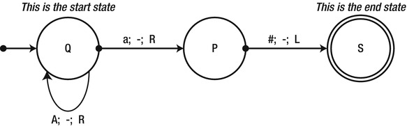
Figure 9-1 . A state diagram of a simple Turing machine. The leftmost arrow points into the initial state, Q. The looped arrow shows that when the machine is in state Q and reads the symbol A, it moves to the right and remains in state Q
When discussing the complexity of algorithms on a Turing machine, there is no need to reason in vague “iterations”—a computation step of a TM is a single state transition (including a transition from a state to itself). For example, when the TM in Figure 9-1 starts with the input “AAAa#” on its tape, it performs exactly four computation steps. We can generalize this to say that, for an input of n ‘A’s followed by “a#”, the machine performs O(n) steps. (Indeed, for such an input of size n, the machine performs exactly n + 2 steps, so the definition of O(n) holds, for example, with the constant c = 3.)
Modeling real-world computation using a Turing machine is quite difficult—it makes for a good exercise in an undergraduate course on automata theory, but has no practical use. The amazing result is that every C# program (and, in fact, every algorithm that can be executed on a modern computer) can be translated—laboriously—to a Turing machine. Roughly speaking, if an algorithm written in C# has runtime complexity O( f (n)), then the same algorithm translated to a Turing machine has runtime complexity of O( f 2(n)). This has very useful implications on analyzing algorithm complexity: if a problem has an efficient algorithm for a Turing machine, then it has an efficient algorithm for a modern computer; if a problem does not have an efficient algorithm for a Turing machine, then it, typically, does not have an efficient algorithm for a modern computer.
Although we could call O(n2) algorithms efficient and any “slower” algorithms inefficient, complexity theory takes a slightly different stance. P is the set of all problems a Turing machine can solve in polynomial time—in other words, if A is a problem in P (with input of size n), then there exists a Turing machine that produces the desired result on its tape within polynomial time (i.e. within O(n k ) steps for some natural number k). In many subfields of complexity theory, problems in P are considered easy—and algorithms that run in polynomial time are considered efficient, even though k and, therefore, the running time can be very large for some algorithms.
All of the algorithms considered so far in this book are efficient if we embrace this definition. Still, some are “very” efficient and others less so, indicating that this separation is not sufficiently subtle. You might even ask whether there are any problems that are not in P, problems that do not have efficient solutions. The answer is a resounding yes—and, in fact, from a theoretical perspective, there are more problems that do not have efficient solutions than problems that do.
First, we consider a problem that a Turing machine cannot solve, regardless of efficiency. Then, we see there are problems a Turing machine can solve, but not in polynomial time. Finally, we turn to problems for which we do not know whether there is a Turing machine that can solve them in polynomial time, but strongly suspect that there is not.
From a mathematical perspective, there are more problems than Turing machines (we say that Turing machines are “countable” and problems are not), which means there must be infinitely many problems that cannot be solved by Turing machines. This class of problems is often called undecidable problems.
WHAT DO YOU MEAN BY "COUNTABLE"?
In mathematics, there are many kinds of “infinite”. It is easy to see that there are an infinite number of Turing machines—after all, you could add a dummy state that does nothing to any Turing machine and obtain a new, larger Turing machine. Similarly, it is easy to see that there are an infinite number problems—this requires a formal definition of a problem (as a “language”) but leads to the same result. However, it is not obvious why there are “more” problems than Turing machines, especially since the number of both is infinite.
The set of Turing machines is said to be countable, because there is a one-to-one correspondence from natural numbers (1, 2, 3, . . .) to Turing machines. It might not be immediately obvious how to construct this correspondence, but it is possible, because Turing machines can be described as finite strings and the set of all finite strings is countable.
However, the set of problems (languages) is not countable, because a one-to-one correspondence from natural numbers to languages does not exist. A possible proof is along the following lines: consider the set of problems corresponding to all real numbers, where, for any real number r, the problem is to print the number or to recognize whether the number has been supplied as input. A well-known result (Cantor’s Theorem) is that the real numbers are uncountable, and, hence, this set of problems is uncountable as well.
To summarize, this seems like an unfortunate conclusion. Not only are there problems that cannot be solved (decided) by a Turing machine, but there are many more such problems than problems that can be solved by a Turing machine. Luckily, a great many problems can be solved by Turing machines, as the incredible evolution of computers in the 20th century shows, theoretical results notwithstanding.
The halting problem, which we now introduce, is undecidable. The problem is as follows: receive as input a program T (or a description of a Turing machine) and an input w to the program; return TRUE if T halts when executed on w and FALSE if it does not halt (enters an infinite loop).
You could even translate this problem to a C# method that accepts a program’s code as a string:
public static bool DoesHaltOnInput(string programCode, string input) { . . . }
. . .or even a C# method that takes a delegate and an input to feed it:
public static bool DoesHaltOnInput(Action< string > program, string input) { . . . }
Although it may appear there is a way to analyze a program and determine whether it halts or not (e.g. by inspecting its loops, its calls to other methods, and so on), it turns out that there is neither a Turing machine nor a C# program that can solve this problem. How does one reach this conclusion? Obviously, to say a Turing machine can solve a problem, we only need to demonstrate the Turing machine—but, to say that there exists no Turing machine to solve a particular problem, it appears that we have to go over all possible Turing machines, which are infinite in number.
As often is the case in mathematics, we use a proof by contradiction. Suppose someone came up with the method DoesHaltOnInput, which tests whether Then we could write the following C# method:
public static void Helper(string programCode, string input) {
  bool doesHalt = DoesHaltOnInput(programCode, input);
  if (doesHalt) {
    while (true) {} //Enter an infinite loop
  }
}
Now all it takes is to call DoesHaltOnInput on the source of the Helper method (the second parameter is meaningless). If DoesHaltOnInput returns true, the Helper method enters an infinite loop; if DoesHaltOnInput returns false, the Helper method does not enter an infinite loop. This contradiction illustrates that the DoesHaltOnInput method does not exist.
![]() Note The halting problem is a humbling result; it demonstrates, in simple terms, that there are limits to the computational ability of our computing devices. The next time you blame the compiler for not finding an apparently trivial optimization or your favorite static analysis tool for giving you false warnings you can see will never occur, remember that statically analyzing a program and acting on the results is often undecidable. This is the case with optimization, halting analysis, determining whether a variable is used, and many other problems that might be easy for a developer given a specific program but cannot be generally solved by a machine.
Note The halting problem is a humbling result; it demonstrates, in simple terms, that there are limits to the computational ability of our computing devices. The next time you blame the compiler for not finding an apparently trivial optimization or your favorite static analysis tool for giving you false warnings you can see will never occur, remember that statically analyzing a program and acting on the results is often undecidable. This is the case with optimization, halting analysis, determining whether a variable is used, and many other problems that might be easy for a developer given a specific program but cannot be generally solved by a machine.
There are many more undecidable problems. Another simple example stems again from the counting argument. There are a countable number of C# programs, because every C# program is a finite combination of symbols. However, there are uncountably many real numbers in the interval [0,1]. Therefore, there must exist a real number that cannot be printed out by a C# program.
Even within the realm of decidable problems—those that can be solved by a Turing machine—there are problems that do not have efficient solutions. Computing a perfect strategy for a game of chess on an n × n chessboard requires time exponential in n, which places the problem of solving the generalized chess game outside of P. (If you like checkers and dislike computer programs playing checkers better than humans, you should take some solace in the fact that generalized checkers is not in P either.)
There are problems, however, that are thought to be less complex, but for which we do not yet have a polynomial algorithm. Some of these problems would prove quite useful in real-life scenarios:
- The traveling salesman problem: Find a path of minimal cost for a salesman who has to visit n different cities.
- The maximum clique problem: Find the largest subset of nodes in a graph such that every two nodes in the subset are connected by an edge.
- The minimum cut problem: Find a way to divide a graph into two subsets of nodes such that there are a minimal number of edges crossing from one subset to the other.
- The Boolean satisfiability problem: Determine whether a Boolean formula of a certain form (such as “A and B or C and not A”) can be satisfied by an assignment of truth values to its variables.
- The cache placement problem: Decide which data to place in cache and which data to evict from cache, given a complete history of memory accesses performed by an application.
These problems belong in another set of problems called NP. The problems in NP are characterized as follows: if A is a problem in NP, then there exists a Turing machine that can verify the solution of A for an input of size n in polynomial time. For example, verifying that a truth assignment to variables is legal and solves the Boolean satisfiability problem is clearly very easy, as well as linear in the number of variables. Similarly, verifying that a subset of nodes is a clique is very easy. In other words, these problems have easily verifiable solutions, but it is not known whether there is a way to efficiently come up with these solutions.
Another interesting facet of the above problems (and many others) is that if any has an efficient solution, then they all have an efficient solution. The reason is that they can be reduced from one to another. Moreover, if any of these problems has an efficient solution, which means that problem is in P, then the entire NP complexity class collapses into P such that P = NP. Arguably the biggest mystery in theoretical computer science today is whether P = NP (most computer scientists believe these complexity classes are not equal).
Problems that have this collapsing effect on P and NP are called NP-complete problems. For most computer scientists, showing that a problem is NP-complete is sufficient to reject any attempts to devise an efficient algorithm for it. Subsequent sections consider some examples of NP-complete problems that have acceptable approximate or probabilistic solutions.
Memoization and Dynamic Programming
Memoization is a technique that preserves the results of intermediate computations if they will be needed shortly afterwards, instead of recomputing them. It can be considered a form of caching. The classic example comes from calculating Fibonacci numbers, which is often one of the first examples used to teach recursion:
public static ulong FibonacciNumber(uint which) {
  if (which == 1 || which == 2) return 1;
  return FibonacciNumber(which-2) + FibonacciNumber(which-1);
}
This method has an appealing look, but its performance is quite appalling. For inputs as small as 45, this method takes a few seconds to complete; finding the 100th Fibonacci number using this approach is simply impractical, as its complexity grows exponentially.
One of the reasons for this inefficiency is that intermediate results are calculated more than once. For example, FibonacciNumber(10) is calculated recursively to find FibonacciNumber(11) and FibonacciNumber(12), and again for FibonacciNumber(12) and FibonacciNumber(13), and so on. Storing the intermediate results in an array can improve this method’s performance considerably:
public static ulong FibonacciNumberMemoization(uint which) {
  if (which == 1 || which == 2) return 1;
  ulong[] array = new ulong[which];
  array[0] = 1; array[1] = 1;
  return FibonacciNumberMemoization(which, array);
}
private static ulong FibonacciNumberMemoization(uint which, ulong[] array) {
  if (array[which-3] == 0) {
    array[which-3] = FibonacciNumberMemoization(which-2, array);
  }
  if (array[which-2] == 0) {
    array[which-2] = FibonacciNumberMemoization(which-1, array);
  }
  array[which-1] = array[which-3] + array[which-2];
  return array[which-1];
}
This version finds the 10,000th Fibonacci number in a small fraction of a second and scales linearly. Incidentally, this calculation can be expressed in even simpler terms by storing only the last two numbers calculated:
public static ulong FibonacciNumberIteration(ulong which) {
  if (which == 1 || which == 2) return 1;
  ulong a = 1, b = 1;
  for (ulong i = 2; i < which; ++i) {
    ulong c = a + b;
    a = b;
    b = c;
  }
  return b;
}
![]() Note It is worth noting that Fibonacci numbers have a closed formula based on the golden ratio (see http://en.wikipedia.org/wiki/Fibonacci_number#Closed-form_expression for details). However, using this closed formula to find an accurate value might involve non-trivial arithmetic.
Note It is worth noting that Fibonacci numbers have a closed formula based on the golden ratio (see http://en.wikipedia.org/wiki/Fibonacci_number#Closed-form_expression for details). However, using this closed formula to find an accurate value might involve non-trivial arithmetic.
The simple idea of storing results required for subsequent calculations is useful in many algorithms that break down a big problem into a set of smaller problems. This technique is often called dynamic programming. We now consider two examples.
The edit distance between two strings is the number of character substitutions (deletions, insertions, and replacements) required to transform one string into the other. For example, the edit distance between “cat” and “hat” is 1 (replace ‘c’ with ‘h’), and the edit distance between “cat” and “groat” is 3 (insert ‘g’, insert ‘r’, replace ‘c’ with ‘o’). Efficiently finding the edit distance between two strings is important in many scenarios, such as error correction and spell checking with replacement suggestions.
The key to an efficient algorithm is breaking down the larger problem into smaller problems. For example, if we know that the edit distance between “cat” and “hat” is 1, then we also know that the edit distance between “cats” and “hat” is 2—we use the sub-problem already solved to devise the solution to the bigger problem. In practice, we wield this technique more carefully. Given two strings in array form, s[1. . .m] and t[1. . .n], the following hold:
- The edit distance between the empty string and t is n, and the edit distance between s and the empty string is m (by adding or removing all characters).
- If s[i] = t[j] and the edit distance between s[1. . .i-1] and t[1. . .j-1] is k, then we can keep the i-th character and the edit distance between s[1. . .i] and t[1. . .j] is k.
- If s[i] ≠ t[j], then the edit distance between s[1. . .i] and t[1. . .j] is the minimum of:
- The edit distance between s[1. . .i] and t[1. . .j-1], +1 to insert t[j];
- The edit distance between s[1. . .i-1] and t[1. . .j], +1 to delete s[i];
- The edit distance between s[1. . .i-1] and t[1. . .j-1], +1 to replace s[i] by t[j].
The following C# method finds the edit distance between two strings by constructing a table of edit distances for each of the substrings and then returning the edit distance in the ultimate cell in the table:
public static int EditDistance(string s, string t) {
  int m = s.Length, n = t.Length;
  int[,] ed = new int[m,n];
  for (int i = 0; i < m; ++i) {
    ed[i,0] = i + 1;
  }
  for (int j = 0; j < n; ++j) {
    ed[0,j] = j + 1;
  }
  for (int j = 1; j < n; ++j) {
    for (int i = 1; i < m; ++i) {
    if (s[i] == t[j]) {
    ed[i,j] = ed[i-1,j-1]; //No operation required
    } else { //Minimum between deletion, insertion, and substitution
    ed[i,j] = Math.Min(ed[i-1,j] + 1, Math.Min(ed[i,j-1] + 1, ed[i-1,j-1] + 1));
    }
    }
  }
  return ed[m-1,n-1];
}
The algorithm fills the edit distances table column-by-column, such that it never attempts to use data not yet calculated. Figure 9-2 illustrates the edit distances table constructed by the algorithm when run on the inputs “stutter” and “glutton”.
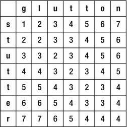
Figure 9-2 . The edit distances table, completely filled out
This algorithm uses O(mn) space and has running time complexity of O(mn). A comparable recursive solution that did not use memoization would have exponential running time complexity and fail to perform adequately even for medium-size strings.
The all-pairs-shortest-paths problem is to find the shortest distances between every two pairs of vertices in a graph. This can be useful for planning factory floors, estimating trip distances between cities, evaluating the required cost of fuel, and many other real-life scenarios. The authors encountered this problem in one of their consulting engagements. This was the problem description provided by the customer (see Sasha Goldshtein’s blog post at http://blog.sashag.net/archive/2010/12/16/all-pairs-shortest-paths-algorithm-in-real-life.aspx for the original story):
- We are implementing a service that manages a set of physical backup devices. There is a set of conveyor belts with intersections and robot arms that manipulate backup tapes across the room. The service gets requests, such as “transfer a fresh tape X from storage cabinet 13 to backup cabinet 89, and make sure to pass through formatting station C or D”.
- When the system starts, we calculate all shortest routes from every cabinet to every other cabinet, including special requests, such as going through a particular computer. This information is stored in a large hashtable indexed by route descriptions and with routes as values.
- System startup with 1,000 nodes and 250 intersections takes more than 30 minutes, and memory consumption reaches a peak of approximately 5GB. This is not acceptable.
First, we observe that the constraint “make sure to pass through formatting computer C or D” does not pose significant additional challenge. The shortest path from A to B going through C is the shortest path from A to C followed by the shortest path from C to B (the proof is almost a tautology).
The Floyd-Warshall algorithm finds the shortest paths between every pair of vertices in the graph and uses decomposition into smaller problems quite similar to what we have seen before. The recursive formula, this time, uses the same observation made above: the shortest path from A to B goes through some vertex V. Then to find the shortest path from A to B, we need to find first the shortest path from A to V and then the shortest path from V to B, and concatenate them together. Because we do not know what V is, we need to consider all possible intermediate vertices—one way to do so is by numbering them from 1 to n.
Now, the length of the shortest path (SP) from vertex i to vertex j using only the vertices 1,. . .,k is given by the following recursive formula, assuming there is no edge from i to j:
SP(i, j, k) = min { SP(i, j, k-1), SP(i, k, k-1) + SP(k, j, k-1) }
To see why, consider the vertex k. Either the shortest path from i to j uses this vertex or it does not. If the shortest path does not use the vertex k, then we do not have to use this vertex and can rely on the shortest path using only the vertices 1,. . .,k-1. If the shortest path uses the vertex k, then we have our decomposition—the shortest path can be sewn together from the shortest path from i to k (that uses only the vertices 1,. . .,k-1) and the shortest path from k to j (that uses only the vertices 1,. . .,k-1). See Figure 9–3 for an example.
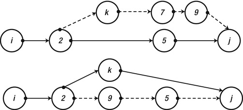
Figure 9-3 . In the upper part of the diagram, the shortest path from i to j (through vertices 2 and 5) does not use the vertex k. Hence, we can restrict ourselves to the shortest path using vertices 1,. . .,k-1. In the lower part, the shortest path from i to j uses vertex k. Hence the shortest path from i to j is the shortest path from i to k, sewn together with the shortest path from k to j
To get rid of the recursive calls, we use memoization—this time we have a three-dimensional table to fill, and, after finding the values of SP for all pairs of vertices and all values of k, we have the solution to the all-pairs-shortest-paths problem.
We can further reduce the amount of storage space by noting that, for every pair of vertices i, j, we do not actually need all the values of k from 1 to n—we need only the minimum value obtained so far. This makes the table two-dimensional and the storage only O(n2). The running time complexity remains O(n3), which is quite incredible considering that we find the shortest path between every two vertices in the graph.
Finally, when filling the table, we need to record for each pair of vertices i, j the next vertex x to which we should proceed if we want to find the actual shortest path between the vertices. The translation of these ideas to C# code is quite easy, as is reconstructing the path based on this last observation:
static short[,] costs;
static short[,] next;

public static void AllPairsShortestPaths(short[] vertices, bool[,] hasEdge) {
  int N = vertices.Length;
  costs = new short[N, N];
  next = new short[N, N];
  for (short i = 0; i < N; ++i) {
    for (short j = 0; j < N; ++j) {
       costs[i, j] = hasEdge[i, j] ? (short)1 : short.MaxValue;
       if (costs[i, j] == 1)
          next[i, j] = −1; //Marker for direct edge
    }
  }
  for (short k = 0; k < N; ++k) {
    for (short i = 0; i < N; ++i) {
       for (short j = 0; j < N; ++j) {
          if (costs[i, k] + costs[k, j] < costs[i, j]) {
             costs[i, j] = (short)(costs[i, k] + costs[k, j]);
                next[i, j] = k;
          }
       }
    }
  }
}
public string GetPath(short src, short dst) {
    if (costs[src, dst] == short.MaxValue) return " < no path > ";
    short intermediate = next[src, dst];
    if (intermediate == −1)
       return "- > "; //Direct path
    return GetPath(src, intermediate) + intermediate + GetPath(intermediate, dst);
}
This simple algorithm improved the application performance dramatically. In a simulation with 300 nodes and an average fan-out of 3 edges from each node, constructing the full set of paths took 3 seconds and answering 100,000 queries about shortest paths took 120ms, with only 600KB of memory used.
This section considers two algorithms that do not offer an accurate solution to the posed problem, but the solution they give can be an adequate approximation. If we look for the maximum value of some function f (x), an algorithm that returns a result that is always within a factor of c of the actual value (which may be hard to find) is called a c-approximation algorithm.
Approximation is especially useful with NP-complete problems, which do not have known polynomial algorithms. In other cases, approximation is used to find solutions more efficiently than by completely solving the problem, sacrificing some accuracy in the process. For example, a O(logn) 2-approximation algorithm may be more useful for large inputs than an O(n3) precise algorithm.
To perform a formal analysis, we need to formalize somewhat the traveling salesman problem referred to earlier. We are given a graph with a weight function w that assigns the graph’s edges positive values—you can think of this weight function as the distance between cities. The weight function satisfies the triangle inequality, which definitely holds if we keep to the analogy of traveling between cities on a Euclidean surface:
For all vertices x, y, z w(x, y) + w(y, z) ≥ w(x, z)
The task, then, is to visit every vertex in the graph (every city on the salesman’s map) exactly once and return to the starting vertex (the company headquarters), making sure the sum of edge weights along this path is minimal. Let wOPT be this minimal weight. (The equivalent decision problem is NP-complete, as we have seen.)
The approximation algorithm proceeds as follows. First, construct a minimal spanning tree (MST) for the graph. Let wMST be the tree’s total weight. (A minimal spanning tree is a subgraph that touches every vertex, does not have cycles, and has the minimum total edge weight of all such trees.)
We can assert that wMST ≤ wOPT, because wOPT is the total weight of a cyclic path that visits every vertex; removing any edge from it produces a spanning tree, and wMST is the total weight of the minimum spanning tree. Armed with this observation, we produce a 2-approximation to wOPT using the minimum spanning tree as follows:
- Construct an MST. There is a known O(n logn) greedy algorithm for this.
- Traverse the MST from its root by visiting every node and returning to the root. The total weight of this path is 2wMST ≤ 2wOPT.
- Fix the resulting path such that no vertex is visited more than once. If the situation in Figure 9-4 arises—the vertex y was visited more than once—then fix the path by removing the edges (x, y) and (y, z) and replacing them with the edge (x, z). This can only decrease the total weight of the path because of the triangle inequality.
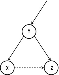
Figure 9-4 . Instead of traversing Y twice, we can replace the path (X, Y, Z) with the path (X, Z)
The result is a 2-approximation algorithm, because the total weight of the path produced is still, at most, double the weight of the optimal path.
We are given a graph and need to find a cut—a grouping of its vertices into two disjoint sets—such that the number of edges crossing between the sets (crossing the cut) is maximal. This is known as the maximum cut problem, and solving it is quite useful for planning in many engineering fields.
We produce a very simple and intuitive algorithm that yields a 2-approximation:
- Divide the vertices into two arbitrary disjoint sets, A and B.
- Find a vertex v in A that has more neighbors in A than in B. If not found, halt.
- Move v from A to B and go back to step 2.
First, let A be a subset of the vertices and v a vertex in A. We denote by degA(v) the number of vertices in A that v has an edge with (i.e. the number of its neighbors in A). Next, given two subsets A, B of the vertices, we denote by e(A, B) the number of edges between vertices in two different sets and by e(A) the number of edges between vertices in the set A.
When the algorithm terminates, for each v in A, it holds that degB(v) ≥ degA(v)—otherwise the algorithm would repeat step 2. Summing over all the vertices, we obtain that e(A, B) ≥ degB(v1) + . . . + degB(vk) ≥ degA(v1) + . . . + degA(vk) ≥ 2e(A), because every edge on the right hand side was counted twice. Similarly, e(A, B) ≥ 2e(B) and, therefore, 2e(A, B) ≥ 2e(A) + 2e(B). From this we obtain 2e(A, B) ≥ e(A, B) + e(A) + e(B), but the right hand side is the total number of edges in the graph. Therefore, the number of edges crossing the cut is at least one-half the total number of edges in the graph. The number of edges crossing the cut cannot be larger than the total number of edges in the graph, so we have a 2-approximation.
Finally, it is worth noting that the algorithm runs for a number of steps that is linear in the number of edges in the graph. Whenever step 2 repeats, the number of edges crossing the cut increases by at least 1, and it is bounded from above by the total number of edges in the graph, so the number of steps is also bounded from above by that number.
When considered approximation algorithms, we were still bound by the requirement of producing a deterministic solution. There are some cases, however, in which introducing a source of randomness into an algorithm can provide probabilistically sound results, although it becomes no longer possible to guarantee absolutely the algorithm’s correctness or bounded running time.
It turns out that a 2-approximation of the maximum cut problem can be obtained by randomly selecting the two disjoint sets (specifically, flipping a coin for each vertex to decide whether it goes into A or B). By probabilistic analysis, the expected number of edges crossing the cut is ½ the total number of edges.
To show that the expected number of edges crossing the cut is ½ the total number of edges, consider the probability that a specific edge (u, v) is crossing the cut. There are four alternatives with equal probability ¼: the edge is in A; the edge is in B; v is in A, and u is in B; and v is in B, and u is in A. Therefore, the probability the edge is crossing the cut is ½.
For an edge e, the expected value of the indicator variable Xe (that is equal to 1 when the edge is crossing the cut) is ½. By linearity of expectation, the expected number of edges in the cut is ½ the number of edges in the graph.
Note that we can no longer trust the results of a single round, but there are derandomization techniques (such as the method of conditional probabilities) that can make success very likely after a small constant number of rounds. We have to prove a bound on the probability that the number of edges crossing the cut is smaller than ½ the number of edges in the graph—there are several probabilistic tools, including Markov’s inequality, that can be used to this end. We do not, however, perform this exercise here.
Finding the prime numbers in a range is an operation we parallelized in Chapter 6, but we never got as far as looking for a considerably better algorithm for testing a single number for primality. This operation is important in applied cryptography. For example, the RSA asymmetric encryption algorithm used ubiquitously on the Internet relies on finding large primes to generate encryption keys.
A simple result from number theory known as Fermat’s little theorem states that, if p is prime, then for all numbers 1 ≤ a ≤ p, the number a p-1 has remainder 1 when divided by p (denoted a p-1 ≡ 1 (mod p)). We can use this idea to devise the following probabilistic primality test for a candidate n:
- Pick a random number a in the interval [1, n], and see if the equality from Fermat’s little theorem holds (i.e. if a p-1 has remainder 1 when divided by p).
- Reject the number as composite, if the equality does not hold.
- Accept the number as prime or repeat step 1 until the desired confidence level is reached, if the equality holds.
For most composite numbers, a small number of iterations through this algorithm detects that it is composite and rejects it. All prime numbers pass the test for any number of repetitions, of course.
Unfortunately, there are infinitely many numbers (called Carmichael numbers) that are not prime but will pass the test for every value of a and any number of iterations. Although Carmichael numbers are quite rare, they are a sufficient cause of concern for improving the Fermat primality test with additional tests that can detect Carmichael numbers. The Miller-Rabin primality test is one example.
For composite numbers that are not Carmichael, the probability of selecting a number a for which the equality does not hold is more than ½. Thus, the probability of wrongly identifying a composite number as prime shrinks exponentially as the number of iterations increases: using a sufficient number of iterations can decrease arbitrarily the probability of accepting a composite number.
Indexing and Compression
When storing large amounts of data, such as indexed web pages for search engines, compressing the data and accessing it efficiently on disk is often more important than sheer runtime complexity. This section considers two simple examples that minimize the amount of storage required for certain types of data, while maintaining efficient access times.
Suppose you have a collection of 50,000,000 positive integers to store on disk and you can guarantee that every integer will fit into a 32-bit int variable. A naïve solution would be to store 50,000,000 32-bit integers on disk, for a total of 200,000,000 bytes. We seek a better alternative that would use significantly less disk space. (One reason for compressing data on disk might be to load it more quickly into memory.)
Variable length encoding is a compression technique suitable for number sequences that contain many small values. Before we consider how it works, we need to guarantee that there will be many small values in the sequence—which currently does not seem to be the case. If the 50,000,000 integers are uniformly distributed in the range [0, 232], then more than 99% will not fit in 3 bytes and require a full 4 bytes of storage. However, we can sort the numbers prior to storing them on disk, and, instead of storing the numbers, store the gaps. This trick is called gap compression and likely makes the numbers much smaller, while still allowing us to reconstruct the original data.
For example, the series (38, 14, 77, 5, 90) is first sorted to (5, 14, 38, 77, 90) and then encoded using gap compression to (5, 9, 24, 39, 13). Note that the numbers are much smaller when using gap compression, and the average number of bits required to store them has gone down significantly. In our case, if the 50,000,000 integers were uniformly distributed in the range [0, 232], then many gaps would very likely fit in a single byte, which can contain values in the range [0, 256].
Next, we turn to the heart of variable byte length encoding, which is just one of a large number of methods in information theory that can compress data. The idea is to use the most significant bit of every byte to indicate whether it is the last byte that encodes a single integer or not. If the bit is off, go on to the next byte to reconstruct the number; if the bit is on, stop and use the bytes read so far to decode the value.
For example, the number 13 is encoded as 10001101—the high bit is on, so this byte contains an entire integer and the rest of it is simply the number 13 in binary. Next, the number 132 is encoded as 00000001`10000100. The first byte has its high bit off, so remember the seven bits 0000001, and the second byte has its high bit on, so append the seven bits 0000000 and obtain 10000100, which is the number 132 in binary. In this example, one of the numbers was stored using just 1 byte, and the other using 2 bytes. Storing the gaps obtained in the previous step using this technique is likely to compress the original data almost four-fold. (You can experiment with randomly generated integers to establish this result.)
To store an index of words that appear on web pages in an efficient way—which is the foundation of a crude search engine—we need to store, for each word, the page numbers (or URLs) in which it appears, compressing the data, while maintaining efficient access to it. In typical settings, the page numbers in which a word appears do not fit in main memory, but the dictionary of words just might.
Storing on disk the page numbers in which dictionary words appear is a task best left to variable length encoding—which we just considered. However, storing the dictionary itself is somewhat more complex. Ideally, the dictionary is a simple array of entries that contain the word itself and a disk offset to the page numbers in which the words appears. To enable efficient access to this data, it should be sorted—this guarantees O(logn) access times.
Suppose each entry is the in-memory representation of the following C# value type, and the entire dictionary is an array of them:
struct DictionaryEntry {
  public string Word;
  public ulong DiskOffset;
}
DictionaryEntry[] dictionary = . . .;
As Chapter 3 illustrates, an array of value types consists solely of the value type instances. However, each value type contains a reference to a string; for n entries, these references, along with the disk offsets, occupy 16n bytes on a 64-bit system. Additionally, the dictionary words themselves take up valuable space, and each dictionary word—stored as a separate string— has an extra 24 bytes of overhead (16 bytes of object overhead + 4 bytes to store the string length + 4 bytes to store the number of characters in the character buffer used internally by the string).
We can considerably decrease the amount of space required to store the dictionary entries by concatenating all dictionary words to a single long string and storing offsets into the string in the DictionaryEntry structure (see Figure 9-5). These concatenated dictionary strings are rarely longer than 224 bytes = 16MB, meaning the index field can be a 3-byte integer instead of an 8-byte memory address:
[StructLayout(LayoutKind.Sequential, Pack = 1, Size = 3)]
struct ThreeByteInteger {
  private byte a, b, c;
  public ThreeByteInteger() {}
  public ThreeByteInteger(uint integer) . . .
  public static implicit operator int(ThreeByteInteger tbi) . . .
}
struct DictionaryEntry {
  public ThreeByteInteger LongStringOffset;
  public ulong    DiskOffset;
}
class Dictionary {
  public DictionaryEntry[] Entries = . . .;
  public string    LongString;
}
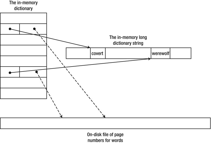
Figure 9-5 . General structure of the in-memory dictionary and string directory
The result is that we maintain binary search semantics over the array—because the entries have uniform size—but the amount of data stored is significantly smaller. We saved almost 24n bytes for the string objects in memory (there is now just one long string) and another 5n bytes for the string references replaced by offset pointers.
Summary
This chapter examines some of the pillars of theoretical computer science, including runtime complexity analysis, computability, algorithm design, and algorithm optimization. As you have seen, algorithm optimization is not restricted to the ivory tower of academia; there are real-life situations where choosing the proper algorithm or using a compression technique can make a considerable performance difference. Specifically, the sections on dynamic programming, index storage, and approximation algorithms contain recipes that you can adapt for your own applications.
The examples in this chapter are not even the tip of the iceberg of complexity theory and algorithms research. Our primary hope is that, by reading this chapter, you learned to appreciate some of the ideas behind theoretical computer science and practical algorithms used by real applications. We know that many .NET developers rarely encounter the need to invent a completely new algorithm, but we still think it is important to understand the taxonomy of the field and have some examples of algorithms on your tool belt.