
![]()
For many years, the processing power of computer systems increased exponentially. Processors have been getting faster with every model, and programs designed to challenge the hardware resources of an expensive workstation were being ported to laptops and handheld devices. This era came to an end several years ago, and today processors are not exponentially increasing in speed; they are exponentially increasing in number. Writing programs to take advantage of multiple processing cores hasn’t been easy when multi-processor systems were rare and expensive, and it hasn’t turned easy today, when even smartphones ship with dual- and quad-core processors.
In this chapter, we shall embark on a whirlwind tour through the world of modern parallel programming in .NET. Although this modest chapter cannot begin to describe all the APIs, frameworks, tools, pitfalls, design patterns, and architectural models that parallel programming is today, no book on performance optimization would be complete without discussing one of the apparently cheapest ways to improve application performance—namely, scaling to multiple processors.
Challenges and Gains
Another challenge of harnessing parallelism is the rising heterogeneity of multi-processor systems. CPU manufacturers take pride in delivering reasonably priced consumer-oriented systems with four or eight processing cores, and high-end server systems with dozens of cores. However, nowadays a mid-range workstation or a high-end laptop often comes equipped with a powerful graphics processing unit (GPU), with support for hundreds of concurrent threads. As if the two kinds of parallelism were not enough, Infrastructure-as-a-Service (IaaS) price drops sprout weekly, making thousand-core clouds accessible in a blink of an eye.
![]() Note Herb Sutter gives an excellent overview of the heterogeneous world that awaits parallelism frameworks in his article “Welcome to the Jungle” (2011). In another article from 2005, “The Free Lunch Is Over,” he shaped the resurgence of interest in concurrency and parallelism frameworks in everyday programming. If you should find yourself hungry for more information on parallel programming than this single chapter can provide, we can recommend the following excellent books on the subject of parallel programming in general and .NET parallelism frameworks in particular: Joe Duffy, “Concurrent Programming on Windows” (Addison-Wesley, 2008); Joseph Albahari, “Threading in C#” (online, 2011). To understand in more detail the operating system’s inner workings around thread scheduling and synchronization mechanisms, Mark Russinovich’s, David Solomon’s, and Alex Ionescu’s “Windows Internals, 5th Edition” (Microsoft Press, 2009) is an excellent text. Finally, the MSDN is a good source of information on the APIs we will see in this chapter, such as the Task Parallel Library.
Note Herb Sutter gives an excellent overview of the heterogeneous world that awaits parallelism frameworks in his article “Welcome to the Jungle” (2011). In another article from 2005, “The Free Lunch Is Over,” he shaped the resurgence of interest in concurrency and parallelism frameworks in everyday programming. If you should find yourself hungry for more information on parallel programming than this single chapter can provide, we can recommend the following excellent books on the subject of parallel programming in general and .NET parallelism frameworks in particular: Joe Duffy, “Concurrent Programming on Windows” (Addison-Wesley, 2008); Joseph Albahari, “Threading in C#” (online, 2011). To understand in more detail the operating system’s inner workings around thread scheduling and synchronization mechanisms, Mark Russinovich’s, David Solomon’s, and Alex Ionescu’s “Windows Internals, 5th Edition” (Microsoft Press, 2009) is an excellent text. Finally, the MSDN is a good source of information on the APIs we will see in this chapter, such as the Task Parallel Library.
The performance gains from parallelism are not to be dismissed lightly. I/O-bound applications can benefit greatly from offloading I/O to separate thread, performing asynchronous I/O to provide higher responsiveness, and scaling by issuing multiple I/O operations. CPU-bound applications with algorithms that yield themselves to parallelization can scale by an order of magnitude on typical consumer hardware by utilizing all available CPU cores or by two orders of magnitude by utilizing all available GPU cores. Later in this chapter you will see how a simple algorithm that performs matrix multiplication is sped up 130-fold by only changing a few lines of code to run on the GPU.
As always, the road to parallelism is laden with pitfalls—deadlocks, race conditions, starvation, and memory corruptions await at every step. Recent parallelism frameworks, including the Task Parallel Library (.NET 4.0) and C++ AMP that we will be using in this chapter, aim to reduce somewhat the complexity of writing parallel applications and harvesting the ripe performance profits.
Why Concurrency and Parallelism?
There are many reasons to introduce multiple threads of control into your applications. This book is dedicated to improving application performance, and indeed most reasons for concurrency and parallelism lie in the performance realm. Here are some examples:
- Issuing asynchronous I/O operations can improve application responsiveness. Most GUI applications have a single thread of control responsible for all UI updates; this thread must never be occupied for a long period of time, lest the UI become unresponsive to user actions.
- Parallelizing work across multiple threads can drive better utilization of system resources. Modern systems, equipped with multiple CPU cores and even more GPU cores can gain an order-of-magnitude increase in performance through parallelization of simple CPU-bound algorithms.
- Performing several I/O operations at once (for example, retrieving prices from multiple travel websites simultaneously, or updating files in several distributed Web repositories) can help drive better overall throughput, because most of the time is spent waiting for I/O operations to complete, and can be used to issue additional I/O operations or perform result processing on operations that have already completed.
From Threads to Thread Pool to Tasks
In the beginning there were threads. Threads are the most rudimentary means of parallelizing applications and distributing asynchronous work; they are the most low-level abstraction available to user-mode programs. Threads offer little in the way of structure and control, and programming threads directly resembles strongly the long-gone days of unstructured programming, before subroutines and objects and agents have gained in popularity.
Consider the following simple task: you are given a large range of natural numbers, and are required to find all the prime numbers in the range and store them in a collection. This is a purely CPU-bound job, and has the appearance of an easily parallelizable one. First, let’s write a naïve version of the code that runs on a single CPU thread:
//Returns all the prime numbers in the range [start, end)
public static IEnumerable < uint > PrimesInRange(uint start, uint end) {
  List < uint > primes = new List < uint > ();
  for (uint number = start; number < end; ++number) {
    if (IsPrime(number)) {
    primes.Add(number);
    }
  }
  return primes;
}
private static bool IsPrime(uint number) {
  //This is a very inefficient O(n) algorithm, but it will do for our expository purposes
  if (number == 2) return true;
  if (number % 2 == 0) return false;
  for (uint divisor = 3; divisor < number; divisor += 2) {
    if (number % divisor == 0) return false;
  }
  return true;
}
Is there anything to improve here? Mayhap the algorithm is so quick that there is nothing to gain by trying to optimize it? Well, for a reasonably large range, such as [100, 200000), the code above runs for several seconds on a modern processor, leaving ample room for optimization.
You may have significant reservations about the efficiency of the algorithm (e.g., there is a trivial optimization that makes it run in O(√n) time instead of linear time), but regardless of algorithmic optimality, it seems very likely to yield well to parallelization. After all, discovering whether 4977 is prime is independent of discovering whether 3221 is prime, so an apparently easy way to parallelize the above code is by dividing the range into a number of chunks and creating a separate thread to deal with each chunk (as illustrated in Figure 6-1). Clearly, we will have to synchronize access to the collection of primes to protect it against corruption by multiple threads. A naïve approach is along the following lines:
public static IEnumerable < uint > PrimesInRange(uint start, uint end) {
  List < uint > primes = new List < uint > ();
  uint range = end - start;
  uint numThreads = (uint)Environment.ProcessorCount; //is this a good idea?
  uint chunk = range / numThreads; //hopefully, there is no remainder
  Thread[] threads = new Thread[numThreads];
  for (uint i = 0; i < numThreads; ++i) {
    uint chunkStart = start + i*chunk;
    uint chunkEnd = chunkStart + chunk;
    threads[i] = new Thread(() = > {
     for (uint number = chunkStart; number < chunkEnd; ++number) {
       if (IsPrime(number)) {
          lock(primes) {
             primes.Add(number);
             }
          }
       }
    });
    threads[i].Start();
  }
  foreach (Thread thread in threads) {
    thread.Join();
  }
  return primes;
}
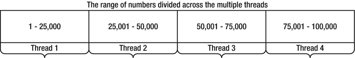
Figure 6-1 . Dividing the range of prime numbers across multiple threads
On an Intel i7 system, the sequential code took ∼ 2950 ms on average to traverse the range [100, 200000), and the parallelized version took ∼ 950 ms on average to do the same. From a system with 8 CPU cores you expect better results, but this particular strain of i7 processors uses HyperThreading, which means there are only 4 physical cores (each physical core hosts two logical cores). A 4× speedup is more reasonable to expect, and we gained a 3× speedup, which is still non-negligible. However, as the Concurrency Profiler’s report in Figures 6-2 and 6-3 shows, some threads finish faster than others, bringing the overall CPU utilization to much lower than 100% (to run the Concurrency Profiler on your applications, consult Chapter 2).
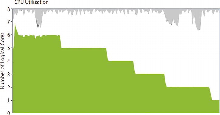
Figure 6-2 . Overall CPU utilization rose to almost 8 logical cores (100%) and then dropped to only one logical core at the end of the run
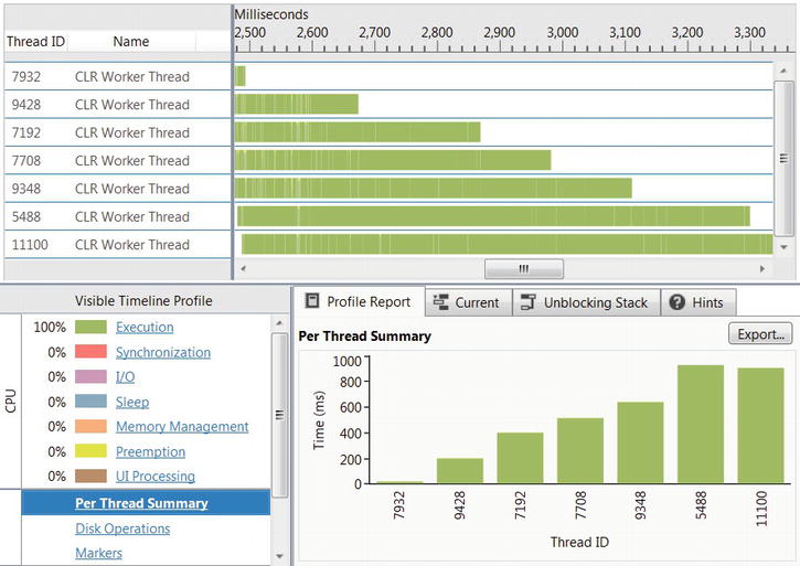
Figure 6-3 . Some threads finished much faster than others. While thread 9428 ran for less than 200ms, thread 5488 ran for more than 800ms
Indeed, this program might run faster than the sequential version (although will not scale linearly), especially if you throw a lot of cores into the mix. This begets several questions, however:
- How many threads are optimal? If the system has eight CPU cores, should we create eight threads?
- How do we make sure that we don’t monopolize system resources or create oversubscription? For example, what if there is another thread in our process that needs to calculate prime numbers, and tries to run the same parallelized algorithm as we do?
- How do the threads synchronize access to the resulting collection? Accessing a List < uint > from multiple threads is unsafe, and will result in data corruption, as we shall see in a subsequent section. However, taking a lock every time we add a prime number to the collection (which is what the naïve solution above does) will prove to be extremely expensive and throttle our ability to scale the algorithm to a further increasing number of processing cores.
- For a small range of numbers, is it worthwhile to spawn several new threads, or perhaps it would be a better idea to execute the entire operation synchronously on a single thread? (Creating and destroying a thread is cheap on Windows, but not as cheap as finding out whether 20 small numbers are prime or composite.)
- How do we make sure that all the threads have an equal amount of work? Some threads might finish more quickly than others, especially those that operate on smaller numbers. For the range [100, 100000) divided into four equal parts, the thread responsible for the range [100, 25075) will finish more than twice as fast as the thread responsible for the range [75025, 100000), because our primality testing algorithm becomes increasingly slower as it encounters large prime numbers.
- How should we deal with exceptions that might arise from the other threads? In this particular case, it would appear that there are no possible errors to come out of the IsPrime method, but in real-world examples the parallelized work could be ridden with potential pitfalls and exceptional conditions. (The CLR’s default behavior is to terminate the entire process when a thread fails with an unhandled exception, which is generally a good idea—fail-fast semantics—but won’t allow the caller of PrimesInRange to deal with the exception at all.)
Good answers to these questions are far from trivial, and developing a framework that allows concurrent work execution without spawning too many threads, that avoids oversubscription and makes sure work is evenly distributed across all threads, that reports errors and results reliably, and that cooperates with other sources of parallelism within the process was precisely the task for the designers of the Task Parallel Library, which we shall deal with next.
From manual thread management, the natural first step was towards thread pools. A thread pool is a component that manages a bunch of threads available for work item execution. Instead of creating a thread to perform a certain task, you queue that task to the thread pool, which selects an available thread and dispatches that task for execution. Thread pools help address some of the problems highlighted above—they mitigate the costs of creating and destroying threads for extremely short tasks, help avoid monopolization of resources and oversubscription by throttling the total number of threads used by the application, and automate decisions pertaining to the optimal number of threads for a given task.
In our particular case, we may decide to break the number range into a significantly larger number of chunks (at the extreme, a chunk per loop iteration) and queue them to the thread pool. An example of this approach for a chunk size of 100 is below:
public static IEnumerable < uint > PrimesInRange(uint start, uint end) {
  List < uint > primes = new List < uint > ();
  const uint ChunkSize = 100;
  int completed = 0;
  ManualResetEvent allDone = new ManualResetEvent(initialState: false);
  uint chunks = (end - start) / ChunkSize; //again, this should divide evenly
  for (uint i = 0; i < chunks; ++i) {
    uint chunkStart = start + i*ChunkSize;
    uint chunkEnd = chunkStart + ChunkSize;
    ThreadPool.QueueUserWorkItem(_ => {
    for (uint number = chunkStart; number < chunkEnd; ++number) {
       if (IsPrime(number)) {
          lock(primes) {
             primes.Add(number);
             }
          }
       }
       if (Interlocked.Increment(ref completed) == chunks) {
          allDone.Set();
       }
    });
  }
  allDone.WaitOne();
  return primes;
}
This version of the code is significantly more scalable, and executes faster than the previous versions we have considered. It improves upon the ∼ 950 ms (for the range [100, 300000)) required for the unsophisticated thread-based version and completes within ∼ 800 ms on average (which is almost a 4× speedup compared to the sequential version). What’s more, CPU usage is at a consistent level of close to 100%, as the Concurrency Profiler report in Figure 6-4 indicates.
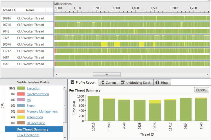
Figure 6-4 . The CLR thread pool used 8 threads (one per logical core) during the program’s execution. Each thread ran for almost the entire duration
As of CLR 4.0, the CLR thread pool consists of several cooperating components. When a thread that doesn’t belong to the thread pool (such as the application’s main thread) dispatches work items to the thread pool, they are enqueued into a global FIFO (first-in-first-out) queue. Each thread pool thread has a local LIFO (last-in-first-out) queue, to which it will enqueue work items created on that thread (see Figure 6-5). When a thread pool thread is looking for work, it begins by consulting its own LIFO queue, and executes work items from it as long as they are available. If a thread’s LIFO queue is exhausted, it will attempt work stealing—consulting the local queues of other threads and taking work items from them, in FIFO order. Finally, if all the local queues are empty, threads will consult the global (FIFO) queue and execute work items from there.
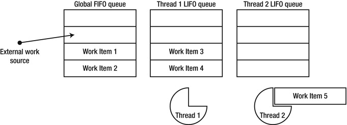
Figure 6-5 . Thread #2 is currently executing work item #5; after completing its execution, it will borrow work from the global FIFO queue. Thread #1 will drain its local queue before tending to any other work
THREAD POOL FIFO AND LIFO SEMANTICS
The reason behind the apparently eccentric FIFO and LIFO queue semantics is the following: when work is enqueued to the global queue, no particular thread has any preference to executing that work, and fairness is the only criterion by which work is selected for execution. This is why FIFO semantics are suitable for the global queue. However, when a thread pool thread queues a work item for execution, it is likely to use the same data and the same instructions as the currently executing work item; that’s why it makes sense to enqueue it in a LIFO queue that belongs to the same thread—it will be executed shortly after the currently executing work item, and take advantage of the CPU data and instruction caches.
Furthermore, accessing work items on the thread’s local queue requires less synchronization and is less likely to encounter contention from other threads than when accessing the global queue. Similarly, when a thread steals work from another thread’s queue, it steals it in FIFO order, so that the LIFO optimization with respect to CPU caches on the original thread’s processor is maintained. This thread pool structure is very friendly towards work item hierarchies, where a single work item enqueued into the global queue will spawn off dozens of additional work items and provide work for several thread pool threads.
As with any abstraction, thread pools take some of the granular control over thread lifetime and work item scheduling away from the application developer. Although the CLR thread pool has some control APIs, such as ThreadPool.SetMinThreads and SetMaxThreads that control the number of threads, it does not have built-in APIs to control the priority of its threads or tasks. More often than not, however, this loss of control is more than compensated by the application’s ability to scale automatically on more powerful systems, and the performance gain from not having to create and destroy threads for short-lived tasks.
Work items queued to the thread pool are extremely inept; they do not have state, can’t carry exception information, don’t have support for asynchronous continuations and cancellation, and don’t feature any mechanism for obtaining a result from a task that has completed. The Task Parallel Library in .NET 4.0 introduces tasks, which are a powerful abstraction on top of thread pool work items. Tasks are the structured alternative to threads and thread pool work items, much in the same way that objects and subroutines were the structured alternative to goto-based assembly language programming.
Task parallelism is a paradigm and set of APIs for breaking down a large task into a set of smaller ones, and executing them on multiple threads. The Task Parallel Library (TPL) has first-class APIs for managing millions of tasks simultaneously (through the CLR thread pool). At the heart of the TPL is the System.Threading.Tasks.Task class, which represents a task. The Task class provides the following capabilities:
- Scheduling work for independent execution on an unspecified thread. (The specific thread to execute a given task is determined by a task scheduler; the default task scheduler enqueues tasks to the CLR thread pool, but there are schedulers that send tasks to a particular thread, such as the UI thread.)
- Waiting for a task to complete and obtaining the result of its execution.
- Providing a continuation that should run as soon as the task completes. (This is often called a callback, but we shall use the term continuation throughout this chapter.)
- Handling exceptions that arise in a single task or even a hierarchy of tasks on the original thread that scheduled them for execution, or any other thread that is interested in the task results.
- Canceling tasks that haven’t started yet, and communicating cancellation requests to tasks that are in the middle of executing.
Because we can think of tasks as a higher-level abstraction on top of threads, we could rewrite the code we had for prime number calculation to use tasks instead of threads. Indeed, it would make the code shorter—at the very least, we wouldn’t need the completed task counter and the ManualResetEvent object to keep track of task execution. However, as we shall see in the next section, the data parallelism APIs provided by the TPL are even more suitable for parallelizing a loop that finds all prime numbers in a range. Instead, we shall consider a different problem.
There is a well-known recursive comparison-based sorting algorithm called QuickSort that yields itself quite easily to parallelization (and has an average case runtime complexity of O(nlog(n)), which is optimal—although scarcely any large framework uses QuickSort to sort anything these days). The QuickSort algorithm proceeds as follows:
public static void QuickSort < T > (T[] items) where T : IComparable < T > {
  QuickSort(items, 0, items.Length);
}
private static void QuickSort < T > (T[] items, int left, int right) where T : IComparable < T > {
  if (left == right) return;
  int pivot = Partition(items, left, right);
  QuickSort(items, left, pivot);
  QuickSort(items, pivot + 1, right);
}
private static int Partition < T > (T[] items, int left, int right) where T : IComparable < T > {
  int pivotPos = . . .; //often a random index between left and right is used
  T pivotValue = items[pivotPos];
  Swap(ref items[right-1], ref items[pivotPos]);
  int store = left;
  for (int i = left; i < right - 1; ++i) {
    if (items[i].CompareTo(pivotValue) < 0) {
    Swap(ref items[i], ref items[store]);
    ++store;
    }
  }
  Swap(ref items[right-1], ref items[store]);
  return store;
}
private static void Swap < T > (ref T a, ref T b) {
  T temp = a;
  a = b;
  b = temp;
}
Figure 6-6 is an illustration of a single step of the Partition method. The fourth element (whose value is 5) is chosen as the pivot. First, it’s moved to the far right of the array. Next, all elements larger than the pivot are propagated towards the right side of the array. Finally, the pivot is positioned such that all elements to its right are strictly larger than it, and all elements to its left are either smaller than or equal to it.
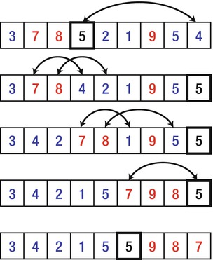
Figure 6-6 . Illustration of a single invocation of the Partition method.
The recursive calls taken by QuickSort at every step must set the parallelization alarm. Sorting the left and right parts of the array are independent tasks, which require no synchronization among them, and the Task class is ideal for expressing this. Below is a first attempt at parallelizing QuickSort using Tasks:
public static void QuickSort < T > (T[] items) where T : IComparable < T > {
  QuickSort(items, 0, items.Length);
}
private static void QuickSort < T > (T[] items, int left, int right) where T : IComparable < T > {
  if (right - left < 2) return;
  int pivot = Partition(items, left, right);
  Task leftTask = Task.Run(() => QuickSort(items, left, pivot));
  Task rightTask = Task.Run(() => QuickSort(items, pivot + 1, right));
  Task.WaitAll(leftTask, rightTask);
}
private static int Partition < T > (T[] items, int left, int right) where T : IComparable < T > {
  //Implementation omitted for brevity
}
The Task.Run method creates a new task (equivalent to calling new Task()) and schedules it for execution (equivalent to the newly created task’s Start method). The Task.WaitAll static method waits for both tasks to complete and then returns. Note that we don’t have to deal with specifying how to wait for tasks to complete, nor when to create threads and when to destroy them.
There is a helpful utility method called Parallel.Invoke, which executes a set of tasks provided to it and returns when all the tasks have completed. This would allow us to rewrite the core of the QuickSort method body with the following:
Parallel.Invoke(
    () => QuickSort(items, left, pivot),
    () => QuickSort(items, pivot + 1, right)
);
Regardless of whether we use Parallel.Invoke or create tasks manually, if we try to compare this version with the straightforward sequential one, we will find that it runs significantly slower, even though it seems to take advantage of all the available processor resources. Indeed, using an array of 1,000,000 random integers, the sequential version ran (on our test system) for ∼ 250 ms and the parallelized version took nearly ∼ 650 ms to complete on average!
The problem is that parallelism needs to be sufficiently coarse-grained; attempting to parallelize the sorting of a three-element array is futile, because the overhead introduced by creating Task objects, scheduling work items to the thread pool, and waiting for them to complete execution overwhelms completely the handful of comparison operations required.
Throttling Parallelism in Recursive Algorithms
How do you propose to throttle the parallelism to prevent this overhead from diminishing any returns from our optimization? There are several viable approaches:
- Use the parallel version as long as the size of the array to be sorted is bigger than a certain threshold (say, 500 items), and switch to the sequential version as soon as it is smaller.
- Use the parallel version as long as the recursion depth is smaller than a certain threshold, and switch to the sequential version as soon as the recursion is very deep. (This option is somewhat inferior to the previous one, unless the pivot is always positioned exactly in the middle of the array.)
- Use the parallel version as long as the number of outstanding tasks (which the method would have to maintain manually) is smaller than a certain threshold, and switch to the sequential version otherwise. (This is the only option when there are no other criteria for limiting parallelism, such as recursion depth or input size.)
Indeed, in the case above, limiting the parallelization for arrays larger than 500 elements produces excellent results on the author’s Intel i7 processor, yielding a 4× improvement in execution time compared to the sequential version. The code changes are quite simple, although the threshold should not be hardcoded in a production-quality implementation:
private static void QuickSort < T > (T[] items, int left, int right) where T : IComparable < T > {
  if (right - left < 2) return;
  int pivot = Partition(items, left, right);
  if (right - left > 500) {
    Parallel.Invoke(
    () => QuickSort(items, left, pivot),
    () => QuickSort(items, pivot + 1, right)
    );
  } else {
    QuickSort(items, left, pivot);
    QuickSort(items, pivot + 1, right);
  }
}
More Examples of Recursive Decomposition
There are many additional algorithms that can be parallelized by applying similar recursive decomposition. In fact, almost all recursive algorithms that split their input into several parts are designed to execute independently on each part and combine the results afterwards. Later in this chapter we shall consider examples that do not succumb so easily for parallelization, but first let’s take a look at a few that do:
- Strassen’s algorithm for matrix multiplication (see http://en.wikipedia.org/wiki/Strassen_algorithm for an overview). This algorithm for matrix multiplication offers better performance than the naïve cubic algorithm we shall see later in this chapter. Strassen’s algorithm recursively decomposes a matrix of size 2n × 2n into four equal block matrices of size 2n-1 × 2n-1, and uses a clever trick that relies on seven multiplications instead of eight to obtain asymptotic running time of ∼ O(n 2.807). As in the QuickSort example, practical implementations of Strassen’s algorithm often fall back to the standard cubic algorithm for small-enough matrices; when parallelizing Strassen’s algorithm using its recursive decomposition, it is even more important to put a threshold on parallelization for smaller matrices.
- Fast Fourier Transform (Cooley-Tukey algorithm, see http://en.wikipedia.org/wiki/Cooley%E2%80%93Tukey_FFT_algorithm). This algorithm computes the DFT (Discrete Fourier Transform) of a vector of length 2n using a recursive decomposition of the vector into two vectors of size 2n-1. Parallelizing this computation is fairly easy, but it is again important to be wary of placing a threshold to the parallelization for sufficiently small vectors.
- Graph traversal (Depth-First Search or Breadth-First Search). As we have seen in Chapter 4, the CLR garbage collector traverses a graph in which objects are vertices and references between objects are edges. Graph traversal using DFS or BFS can benefit greatly from parallelization as well as other recursive algorithms we have considered; however, unlike QuickSort or FFT, when parallelizing branches of the graph traversal it is difficult to estimate in advance the amount of work a recursive call represents. This difficulty requires heuristics to decide how the search space should be partitioned to multiple threads: we have seen that the server GC flavor performs this partitioning rather crudely, based on the separate heaps from which each processor allocates objects.
If you are looking for more examples to practice your parallel programming skills, consider also Karatsuba’s multiplication algorithm that relies on recursive decomposition to multiply n-digit numbers in ∼ O(n 1.585) operations; merge sort that relies on recursive decomposition for sorting, similarly to QuickSort; and numerous dynamic programming algorithms, which often require advanced tricks to employ memoization in different branches of the parallel computation (we will examine one example later).
We haven’t tapped into the full power of the Task class yet. Suppose we wanted to handle exceptions that could arise from the recursive invocations of QuickSort down the line, and provide support for canceling the entire sort operation if it hasn’t completed yet.
The task execution environment provides the infrastructure for marshaling exceptions that arise within the task back to any thread deemed appropriate to receive it. Suppose that one of the recursive invocations of the QuickSort tasks encountered an exception, perhaps because we didn’t consider the array bounds carefully and introduced an off-by-one error to either side of the array. This exception would arise on a thread pool thread, a thread that is not under our explicit control and that does not allow any overarching exception handling behavior. Fortunately, the TPL will catch the exception and store it within the Task object for later propagation.
The exception that arose within a task will be rethrown (wrapped in an AggregateException object) when the program attempts to wait for the task to complete (using the Task.Wait instance method) or to retrieve its result (using the Task.Result property). This allows automatic and centralized exception handling within the code that created the task, and does not require manual propagation of errors to a central location and synchronization of error-reporting activities. The following minimal code example demonstrates the exception-handling paradigm in the TPL:
int i = 0;
Task < int > divideTask = Task.Run(() = > { return 5/i; });
try {
  Console.WriteLine(divideTask.Result); //accessing the Result property eventually throws
} catch (AggregateException ex) {
  foreach (Exception inner in ex.InnerExceptions) {
    Console.WriteLine(inner.Message);
  }
}
![]() Note When creating a task from within the body of an existing task, the TaskCreationOptions.AttachedToParent enumeration value establishes a relationship between the new child task and its parent task in which it was created. We will see later in this chapter that parent–child relationships between tasks affect cancellation, continuations, and debugging aspects of task execution. As far as exception handling is concerned, however, waiting for the parent task to complete implies waiting for all the child tasks to complete, and any exceptions from the child tasks are propagated to the parent task as well. This is why the TPL throws an AggregateException instance, which contains a hierarchy of exceptions that may have arisen from a hierarchy of tasks.
Note When creating a task from within the body of an existing task, the TaskCreationOptions.AttachedToParent enumeration value establishes a relationship between the new child task and its parent task in which it was created. We will see later in this chapter that parent–child relationships between tasks affect cancellation, continuations, and debugging aspects of task execution. As far as exception handling is concerned, however, waiting for the parent task to complete implies waiting for all the child tasks to complete, and any exceptions from the child tasks are propagated to the parent task as well. This is why the TPL throws an AggregateException instance, which contains a hierarchy of exceptions that may have arisen from a hierarchy of tasks.
Cancellation of existing work is another matter to consider. Suppose that we have a hierarchy of tasks, such as the hierarchy created by QuickSort if we used the TaskCreationOptions.AttachedToParent enumeration value. Even though there may be hundreds of tasks running simultaneously, we might want to provide the user with cancellation semantics, e.g. if the sorted data is no longer required. In other scenarios, cancellation of outstanding work might be an integral part of the task execution. For example, consider a parallelized algorithm that looks up a node in a graph using DFS or BFS. When the desired node is found, the entire hierarchy of tasks performing the lookup should be recalled.
Canceling tasks involves the CancellationTokenSource and CancellationToken types, and is performed cooperatively. In other words, if a task’s execution is already underway, it cannot be brutally terminated using TPL’s cancellation mechanisms. Cancellation of already executing work requires cooperation from the code executing that work. However, tasks that have not begun executing yet can be cancelled completely without any malignant consequences.
The following code demonstrates a binary tree lookup where each node contains a potentially long array of elements that needs to be linearly traversed; the entire lookup can be cancelled by the caller using the TPL’s cancellation mechanisms. On the one hand, unstarted tasks will be cancelled automatically by the TPL; on the other hand, tasks that have already started will periodically monitor their cancellation token for cancellation instructions and stop cooperatively when required.
public class TreeNode < T > {
  public TreeNode < T > Left, Right;
  public T[] Data;
}
public static void TreeLookup < T > (
  TreeNode < T > root, Predicate < T > condition, CancellationTokenSource cts) {
  if (root == null) {
    return;
  }
  //Start the recursive tasks, passing to them the cancellation token so that they are
  //cancelled automatically if they haven't started yet and cancellation is requested
  Task.Run(() => TreeLookup(root.Left, condition, cts), cts.Token);
  Task.Run(() => TreeLookup(root.Right, condition, cts), cts.Token);
  foreach (T element in root.Data) {
    if (cts.IsCancellationRequested) break; //abort cooperatively
    if (condition(element)) {
    cts.Cancel(); //cancels all outstanding work
    //Do something with the interesting element
    }
  }
}
//Example of calling code:
CancellationTokenSource cts = new CancellationTokenSource();
Task.Run(() = > TreeLookup(treeRoot, i = > i % 77 == 0, cts);
//After a while, e.g. if the user is no longer interested in the operation:
cts.Cancel();
Inevitably, there will be examples of algorithms where an easier way of expressing parallelism should be desirable. Consider the primality testing example with which we started. We could break the range manually into chunks, create a task for each chunk, and wait for all the tasks to complete. In fact, there is an entire family of algorithms in which there is a range of data to which a certain operation is applied. These algorithms mandate a higher-level abstraction than task parallelism. We now turn to this abstraction.
Whilst task parallelism dealt primarily with tasks, data parallelism aims to remove tasks from direct view and replace them by a higher-level abstraction—parallel loops. In other words, the source of parallelism is not the algorithm’s code, but rather the data on which it operates. The Task Parallel Library offers several APIs providing data parallelism.
Parallel.For and Parallel.ForEach
for and foreach loops are often excellent candidates for parallelization. Indeed, since the dawn of parallel computing, there have been attempts to parallelize such loops automatically. Some attempts have gone the way of language changes or language extensions, such as the OpenMP standard (which introduced directives such as #pragma omp parallel for to parallelize for loops). The Task Parallel Library provides loop parallelism through explicit APIs, which are nonetheless very close to their language counterparts. These APIs are Parallel.For and Parallel.ForEach, matching as closely as possible the behavior of for and foreach loops in the language.
Returning to the example of parallelizing primality testing, we had a loop iterating over a large range of numbers, checking each one for primality and inserting it into a collection, as follows:
for (int number = start; number < end; ++number) {
  if (IsPrime(number)) {
    primes.Add(number);
  }
}
Converting this code to use Parallel.For is almost a mechanical task, although synchronizing access to the collection of primes warrants some caution (and there exist much better approaches, such as aggregation, that we consider later):
Parallel.For(start, end, number => {
  if (IsPrime(number)) {
    lock(primes) {
    primes.Add(number);
    }
  }
});
By replacing the language-level loop with an API call we gain automatic parallelization of the loop’s iterations. Moreover, the Parallel.For API is not a straightforward loop that generates a task per iteration, or a task for each hard-coded chunk-sized part of the range. Instead, Parallel.For adapts slowly to the execution pace of individual iterations, takes into account the number of tasks currently executing, and prevents too-granular behavior by dividing the iteration range dynamically. Implementing these optimizations manually is not trivial, but you can apply specific customizations (such as controlling the maximum number of concurrently executing tasks) using another overload of Parallel.For that takes a ParallelOptions object or using a custom partitioner to determine how the iteration ranges should be divided across different tasks.
A similar API works with foreach loops, where the data source may not be fully enumerated when the loop begins, and in fact may not be finite. Suppose that we need to download from the Web a set of RSS feeds, specified as an IEnumerable < string>. The skeleton of the loop would have the following shape:
IEnumerable < string > rssFeeds = . . .;
WebClient webClient = new WebClient();
foreach (string url in rssFeeds) {
  Process(webClient.DownloadString(url));
}
This loop can be parallelized by the mechanical transformation where the foreach loop is replaced by an API call to Parallel.ForEach. Note that the data source (the rssFeeds collection) need not be thread-safe, because Parallel.ForEach will use synchronization when accessing it from several threads.
IEnumerable < string > rssFeeds = . . .; //The data source need
notbe thread-safe
WebClient webClient = new WebClient();
Parallel.ForEach(rssFeeds, url => {
  Process(webClient.DownloadString(url));
});
![]() Note You can voice a concern about performing an operation on an infinite data source. It turns out, however, that it is quite convenient to begin such an operation and expect to terminate it early when some condition is satisfied. For example, consider an infinite data source such as all the natural numbers (specified in code by a method that returns IEnumerable < BigInteger>). We can write and parallelize a loop that looks for a number whose digit sum is 477 but is not divisible by 133. Hopefully, there is such a number, and our loop will terminate.
Note You can voice a concern about performing an operation on an infinite data source. It turns out, however, that it is quite convenient to begin such an operation and expect to terminate it early when some condition is satisfied. For example, consider an infinite data source such as all the natural numbers (specified in code by a method that returns IEnumerable < BigInteger>). We can write and parallelize a loop that looks for a number whose digit sum is 477 but is not divisible by 133. Hopefully, there is such a number, and our loop will terminate.
Parallelizing loops it not as simple as it may seem from the above discussion. There are several “missing” features we need to consider before we fasten this tool assuredly to our belt. For starters, C# loops have the break keyword, which can terminate a loop early. How can we terminate a loop that has been parallelized across multiple threads, where we don’t even know which iteration is currently executing on threads other than our own?
The ParallelLoopState class represents the state of a parallel loop’s execution, and allows breaking early from a loop. Here is a simple example:
int invitedToParty = 0;
Parallel.ForEach(customers, (customer, loopState) = > {
  if (customer.Orders.Count > 10 && customer.City == "Portland") {
    if (Interlocked.Increment(ref invitedToParty) > = 25) {
    loopState.Stop(); //no attempt will be made to execute any additional iterations
    }
  }
});
Note that the Stop method does not guarantee that the last iteration to execute is the one that called it—iterations that have already started executing will run to completion (unless they poll the ParallelLoopState.ShouldExitCurrentIteration property). However, no additional iterations that have been queued will begin to execute.
One of the drawbacks of ParallelLoopState.Stop is that it does not guarantee that all iterations up to a certain one have executed. For example, if there are 1,000 customers, it is possible that customers 1–100 have been processed completely, customers 101–110 have not been processed at all, and customer 111 was the last to be processed before Stop was called. If you would like to guarantee that all iterations before a certain iteration will have executed (even if they haven’t started yet!), you should use the ParallelLoopState.Break method instead.
Possibly the highest level of abstraction for parallel computation is that where you declare: “I want this code to run in parallel”, and leave the rest for the framework to implement. This is what Parallel LINQ is about. But first, a short refresher on LINQ is due. LINQ (Language INtegrated Query) is a framework and a set of language extensions introduced in C# 3.0 and .NET 3.5, blurring the line between imperative and declarative programming where iterating over data is concerned. For example, the following LINQ query retrieves from a data source called customers—which might be an in-memory collection, a database table, or a more exotic origin—the names and ages of the Washington-based customers who have made at least three over $10 purchases over the last ten months, and prints them to the console:
var results = from customer in customers
          where customer.State == "WA"
          let custOrders = (from order in orders
          where customer.ID == order.ID
          select new { order.Date, order.Amount })
          where custOrders.Count(co => co.Amount >= 10 &&
                   co.Date >= DateTime.Now.AddMonths(−10)) >= 3
          select new { customer.Name, customer.Age };
foreach (var result in results) {
  Console.WriteLine("{0} {1}", result.Name, result.Age);
}
The primary thing to note here is that most of the query is specified declaratively—quite like an SQL query. It doesn’t use loops to filter out objects or to group together objects from different data sources. Often enough, you shouldn’t worry about synchronizing different iterations of the query, because most LINQ queries are purely functional and have no side effects—they convert one collection (IEnumerable < T>) to another without modifying any additional objects in the process.
To parallelize the execution of the above query, the only code change required is to modify the source collection from a general IEnumerable < T > to a ParallelQuery < T>. The AsParallel extension method takes care of this, and allows the following elegant syntax:
var results = from customer in customers.AsParallel()
    where customer.State == "WA"
    let custOrders = (from order in orders
    where customer.ID == order.ID
    select new { order.Date, order.Amount })
    where custOrders.Count(co => co.Amount >= 10 &&
    co.Date > = DateTime.Now.AddMonths(−10)) >= 3
    select new { customer.Name, customer.Age };
foreach (var result in results) {
  Console.WriteLine("{0} {1}", result.Name, result.Age);
}
PLINQ uses a three-stage processing pipeline to execute parallel queries, as illustrated in Figure 6-7. First, PLINQ decides how many threads should be used to parallelize the query’s execution. Next, the worker threads retrieve chunks of work from the source collection, ensuring that it is accessed under a lock. Each thread proceeds to execute its work items independently, and the results are queued locally within each thread. Finally, all the local results are buffered into a single result collection, which is polled by a foreach loop in the above example.
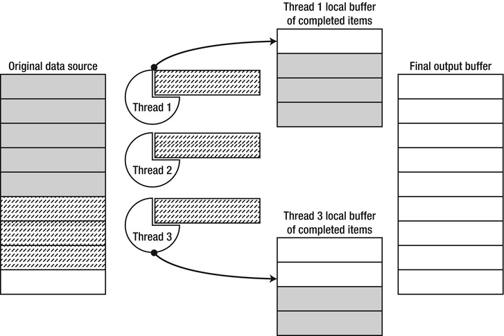
Figure 6-7 . Work item execution in PLINQ. Solid grey work items have been completed and placed in thread-local buffers, from which they are subsequently moved to the final output buffer available to the caller. Dashed work items are currently being executed
The primary advantage of PLINQ compared to Parallel.ForEach stems from the fact that PLINQ automatically handles aggregation of temporary processing results locally within each thread that executes the query. When using Parallel.ForEach to find prime numbers, we had to access a global collection of prime numbers to aggregate the results (and later in this chapter we will consider an optimization that uses aggregation). This global access required continuous synchronization and introduced a significant overhead. We could accomplish the same result by using PLINQ, as follows:
List < int > primes = (from n in Enumerable.Range(3, 200000).AsParallel()
    where IsPrime(n)
    select n).ToList();
//Could have used ParallelEnumerable.Range instead of Enumerable.Range(. . .).AsParallel()
CUSTOMIZING PARALLEL LOOPS AND PLINQ
Parallel loops (Parallel.For and Parallel.ForEach) and PLINQ have several customization APIs, which make them extremely flexible and close in richness and expressiveness to the explicit task parallelism APIs we have considered previously. The parallel loop APIs accept a ParallelOptions object with various properties, whereas PLINQ relies on additional methods of ParallelQuery < T>. These options include:
- Limiting the degree of parallelism (the number of tasks that would be allowed to execute concurrently)
- Providing a cancellation token for canceling the parallel execution
- Forcing output ordering of a parallel query
- Controlling output buffering (merge mode) of a parallel query
With parallel loops, it is most common to limit the degree of parallelism using the ParallelOptions class, whereas with PLINQ, you would often customize the query’s merge mode and ordering semantics. For more information on these customization options, consult the MSDN documentation.
So far, we considered rich APIs that allow a variety of parallelism solutions to be expressed using the classes and methods of the Task Parallel Library. However, other parallel programming environments sometimes rely on language extensions to obtain even better expressiveness where APIs are clumsy or insufficiently concise. In this section we will see how C# 5 adapts to the challenges of the concurrent programming world by providing a language extension to express continuations more easily. But first, we must consider continuations in the asynchronous programming world.
Often enough, you would want to associate a continuation (or callback) with a specific task; the continuation should be executed when the task completes. If you have control of the task—i.e., you schedule it for execution—you can embed the callback in the task itself, but if you receive the task from another method, an explicit continuation API is desirable. The TPL offers the ContinueWith instance method and ContinueWhenAll/ContinueWhenAny static methods (self-explanatory) to control continuations in several settings. The continuation may be scheduled only in specific circumstances (e.g., only when the task ran to completion or only when the task has encountered an exception), and may be scheduled on a particular thread or thread group using the TaskScheduler API. Below are some examples of the various APIs:
Task < string > weatherTask = DownloadWeatherInfoAsync(. . .);
weatherTask.ContinueWith(_ => DisplayWeather(weatherTask.Result), TaskScheduler.Current);
Task left = ProcessLeftPart(. . .);
Task right = ProcessRightPart(. . .);
TaskFactory.ContinueWhenAll(
  new Task[] { left, right },
  CleanupResources
);
TaskFactory.ContinueWhenAny(
  new Task[] { left, right },
  HandleError,
  TaskContinuationOptions.OnlyOnFaulted
);
Continuations are a reasonable way to program asynchronous applications, and are very valuable when performing asynchronous I/O in a GUI setting. For example, to ensure that Windows 8 Metro-style applications maintain a responsive user interface, the WinRT (Windows Runtime) APIs in Windows 8 offer only asynchronous versions of all operations that might run for longer than 50 milliseconds. With multiple asynchronous calls chained together, nested continuations become somewhat clumsy, as the following example may demonstrate:
//Synchronous version:
private void updateButton_Clicked(. . .) {
  using (LocationService location = new LocationService())
  using (WeatherService weather = new WeatherService()) {
    Location loc = location.GetCurrentLocation();
    Forecast forecast = weather.GetForecast(loc.City);
    MessageDialog msg = new MessageDialog(forecast.Summary);
    msg.Display();
  }
}
//Asynchronous version:
private void updateButton_Clicked(. . .) {
  TaskScheduler uiScheduler = TaskScheduler.Current;
  LocationService location = new LocationService();
  Task < Location > locTask = location.GetCurrentLocationAsync();
  locTask.ContinueWith(_ => {
    WeatherService weather = new WeatherService();
    Task < Forecast > forTask = weather.GetForecastAsync(locTask.Result.City);
    forTask.ContinueWith(__ => {
       MessageDialog message = new MessageDialog(forTask.Result.Summary);
       Task msgTask = message.DisplayAsync();
       msgTask.ContinueWith(___ => {
          weather.Dispose();
          location.Dispose();
       });
    }, uiScheduler);
  });
}
This deep nesting is not the only peril of explicit continuation-based programming. Consider the following synchronous loop that requires conversion to an asynchronous version:
//Synchronous version:
private Forecast[] GetForecastForAllCities(City[] cities) {
  Forecast[] forecasts = new Forecast[cities.Length];
  using (WeatherService weather = new WeatherService()) {
    for (int i = 0; i < cities.Length; ++i) {
    forecasts[i] = weather.GetForecast(cities[i]);
    }
  }
  return forecasts;
}
//Asynchronous version:
private Task < Forecast[] > GetForecastsForAllCitiesAsync(City[] cities) {
  if (cities.Length == 0) {
    return Task.Run(() = > new Forecast[0]);
  }
  WeatherService weather = new WeatherService();
  Forecast[] forecasts = new Forecast[cities.Length];
  return GetForecastHelper(weather, 0, cities, forecasts).ContinueWith(_ => forecasts);
}
private Task GetForecastHelper( WeatherService weather, int i, City[] cities, Forecast[] forecasts) {
  if (i >= cities.Length) return Task.Run(() => { });
  Task < Forecast > forecast = weather.GetForecastAsync(cities[i]);
  forecast.ContinueWith(task => {
    forecasts[i] = task.Result;
    GetForecastHelper(weather, i + 1, cities, forecasts);
  });
  return forecast;
}
Converting this loop requires completely rewriting the original method and scheduling a continuation that essentially executes the next iteration in a fairly unintuitive and recursive manner. This is something the C# 5 designers have chosen to address on the language level by introducing two new keywords, async and await.
An async method must be marked with the async keyword and may return void, Task, or Task < T>. Within an async method, the await operator can be used to express a continuation without using the ContinueWith API. Consider the following example:
private async void updateButton_Clicked(. . .) {
  using (LocationService location = new LocationService()) {
    Task < Location > locTask = location.GetCurrentLocationAsync();
    Location loc = await locTask;
    cityTextBox.Text = loc.City.Name;
  }
}
In this example, the await locTask expression provides a continuation to the task returned by GetCurrentLocationAsync. The continuation’s body is the rest of the method (starting from the assignment to the loc variable), and the await expression evaluates to what the task returns, in this case—a Location object. Moreover, the continuation is implicitly scheduled on the UI thread, which is something we had to explicitly take care of earlier using the TaskScheduler API.
The C# compiler takes care of all the relevant syntactic features associated with the method’s body. For example, in the method we just wrote, there is a try. . .finally block hidden behind the using statement. The compiler rewrites the continuation such that the Dispose method on the location variable is invoked regardless of whether the task completed successfully or an exception occurred.
This smart rewriting allows almost trivial conversion of synchronous API calls to their asynchronous counterparts. The compiler supports exception handling, complex loops, recursive method invocation—language constructs that are hard to combine with the explicit continuation-passing APIs. For example, here is the asynchronous version of the forecast-retrieval loop that caused us trouble earlier:
private async Task < Forecast[] > GetForecastForAllCitiesAsync(City[] cities) {
  Forecast[] forecasts = new Forecast[cities.Length];
  using (WeatherService weather = new WeatherService()) {
    for (int i = 0; i < cities.Length; ++i) {
    forecasts[i] = await weather.GetForecastAsync(cities[i]);
    }
  }
  return forecasts;
}
Note that the changes are minimal, and the compiler handles the details of taking the forecasts variable (of type Forecast[]) our method returns and creating the Task < Forecast[] > scaffold around it.
With only two simple language features (whose implementation is everything but simple!), C# 5 dramatically decreases the barrier of entry for asynchronous programming, and makes it easier to work with APIs that return and manipulate tasks. Furthermore, the language implementation of the await operator is not wed to the Task Parallel Library; native WinRT APIs in Windows 8 return IAsyncOperation < T > and not Task instances (which are a managed concept), but can still be awaited, as in the following example, which uses a real WinRT API:
using Windows.Devices.Geolocation;
. . .
private async void updateButton_Clicked(. . .) {
  Geolocator locator = new Geolocator();
  Geoposition position = await locator.GetGeopositionAsync();
  statusTextBox.Text = position.CivicAddress.ToString();
}
So far in this chapter, we have considered fairly simple examples of algorithms that were subjected to parallelization. In this section, we will briefly inspect a few advanced tricks that you may find useful when dealing with real-world problems; in several cases we may be able to extract a performance gain from very surprising places.
The first optimization to consider when parallelizing loops with shared state is aggregation (sometimes called reduction). When using shared state in a parallel loop, scalability is often lost because of synchronization on the shared state access; the more CPU cores are added to the mix, the smaller the gains because of the synchronization (this phenomenon is a direct corollary of Amdahl’s Law, and is often called The Law of Diminishing Returns). A big performance boost is often available from aggregating local state within each thread or task that executes the parallel loop, and combining the local states to obtain the eventual result at the end of the loop’s execution. TPL APIs that deal with loop execution come equipped with overloads to handle this kind of local aggregation.
For example, consider the prime number computation we implemented earlier. One of the primary hindrances to scalability was the need to insert newly discovered prime numbers into a shared list, which required synchronization. Instead, we can use a local list in each thread, and aggregate the lists together when the loop completes:
List < int > primes = new List < int > ();
Parallel.For(3, 200000,
  () => new List < int > (), //initialize the local copy
  (i, pls, localPrimes) => { //single computation step, returns new local state
    if (IsPrime(i)) {
    localPrimes.Add(i); //no synchronization necessary, thread-local state
    }
    return localPrimes;
  },
  localPrimes => { //combine the local lists to the global one
    lock(primes) { //synchronization is required
    primes.AddRange(localPrimes);
    }
  }
);
In the example above, the number of locks taken is significantly smaller than earlier—we only need to take a lock once per thread that executes the parallel loop, instead of having to take it per each prime number we discovered. We did introduce an additional cost of combining the lists together, but this cost is negligible compared to the scalability gained by local aggregation.
Another source of optimization is loop iterations that are too small to be parallelized effectively. Even though the data parallelism APIs chunk multiple iterations together, there may be loop bodies that are so quick to complete that they are dominated by the delegate invocation required to call the loop body for each iteration. In this case, the Partitioner API can be used to extract manually chunks of iterations, minimizing the number of delegate invocations:
Parallel.For(Partitioner.Create(3, 200000), range => { //range is a Tuple < int,int>
  for (int i = range.Item1; i < range.Item2; ++i) . . . //loop body with no delegate invocation
});
For more information on custom partitioning, which is as well an important optimization available to data-parallel programs, consult the MSDN article “Custom Partitioners for PLINQ and TPL”, at http://msdn.microsoft.com/en-us/library/dd997411.aspx.
Finally, there are applications which can benefit from custom task schedulers. Some examples include scheduling work on the UI thread (something we have already done using TaskScheduler.Current to queue continuations to the UI thread), prioritizing tasks by scheduling them to a higher-priority scheduler, and affinitizing tasks to a particular CPU by scheduling them to a scheduler that uses threads with a specific CPU affinity. The TaskScheduler class can be extended to create custom task schedulers. For an example of a custom task scheduler, consult the MSDN article “How to: Create a Task Scheduler That Limits the Degree of Concurrency”, at http://msdn.microsoft.com/en-us/library/ee789351.aspx.
Synchronization
A treatment of parallel programming warrants at least a cursory mention of the vast topic of synchronization. In the simple examples considered throughout this text, we have seen numerous cases of multiple threads accessing a shared memory location, be it a complex collection or a single integer. Aside from read-only data, every access to a shared memory location requires synchronization, but not all synchronization mechanisms have the same performance and scalability costs.
Before we begin, let’s revisit the need for synchronization when accessing small amounts of data. Modern CPUs can issue atomic reads and writes to memory; for example, a write of a 32 bit integer always executes atomically. This means that if one processor writes the value 0xDEADBEEF to a memory location previously initialized with the value 0, another processor will not observe the memory location with a partial update, such as 0xDEAD0000 or 0x0000BEEF. Unfortunately, the same thing is not true of larger memory locations; for example, even on a 64 bit processor, writing 20 bytes into memory is not an atomic operation and cannot be performed atomically.
However, even when accessing a 32 bit memory location but issuing multiple operations, synchronization problems arise immediately. For example, the operation ++i (where i is a stack variable of type int) is typically translated to a sequence of three machine instructions:
mov eax, dword ptr [ebp-64] ;copy from stack to register
inc eax ;increment value in register
mov dword ptr [ebp-64], eax ;copy from register to stack
Each of these instructions executes atomically, but without additional synchronization it is possible for two processors to execute parts of the instruction sequence concurrently, resulting in lost updates. Suppose that the variable’s initial value was 100, and examine the following execution history:
Processor #1 Processor #2
mov eax, dword ptr [ebp-64]
    mov eax, dword ptr [ebp-64] inc eax
inc eax
mov dword ptr [ebp-64], eax
    mov dword ptr [ebp-64], eax
In this case, the variable’s eventual value will be 101, even though two processors have executed the increment operation and should have brought it to 102. This race condition—which is hopefully obvious and easily detectable—is a representative example of the situations that warrant careful synchronization.
OTHER DIRECTIONS
Many researchers and programming language designers do not believe that the situation governing shared memory synchronization can be addressed without changing completely the semantics of programming languages, parallelism frameworks, or processor memory models. There are several interesting directions in this area:
- Transactional memory in hardware or software suggests an explicit or implicit isolation model around memory operations and rollback semantics for series of memory operations. Currently, the performance cost of such approaches impedes their wide adoption in mainstream programming languages and frameworks.
- Agent-based languages bake a concurrency model deep into the language and require explicit communication between agents (objects) in terms of message-passing instead of shared memory access.
- Message-passing processor and memory architectures organize the system using a private-memory paradigm, where access to a shared memory location must be explicit through message-passing at the hardware level.
Throughout the rest of this section, we shall assume a more pragmatic view and attempt to reconcile the problems of shared memory synchronization by offering a set of synchronization mechanisms and patterns. However, the authors firmly believe that synchronization is more difficult than it should be; our shared experience demonstrates that a large majority of difficult bugs in software today stem from the simplicity of corrupting shared state by improperly synchronizing parallel programs. We hope that in a few years—or decades—the computing community will come up with somewhat better alternatives.
One approach to synchronization places the burden on the operating system. After all, the operating system provides the facilities for creating and managing threads, and assumes full responsibility for scheduling their execution. It is then natural to expect from it to provide a set of synchronization primitives. Although we will discuss Windows synchronization mechanisms shortly, this approach begs the question of how the operating system implements these synchronization mechanisms. Surely Windows itself is in need of synchronizing access to its internal data structures—even the data structures representing other synchronization mechanisms—and it cannot implement synchronization mechanisms by deferring to them recursively. It also turns out that Windows synchronization mechanisms often require a system call (user-mode to kernel-mode transition) and thread context switch to ensure synchronization, which is relatively expensive if the operations that require synchronization are very cheap (such as incrementing a number or inserting an item into a linked list).
All the processor families on which Windows can run implement a hardware synchronization primitive called Compare-And-Swap (CAS). CAS has the following semantics (in pseudo-code), and executes atomically:
WORD CAS(WORD* location, WORD value, WORD comparand) {
  WORD old = *location;
  if (old == comparand) {
    *location = value;
  }
  return old;
}
Simply put, CAS compares a memory location with a provided value. If the memory location contains the provided value, it is replaced by another value; otherwise, it is unchanged. In any case, the content of the memory location prior to the operation is returned.
For example, on Intel x86 processors, the LOCK CMPXCHG instruction implements this primitive. Translating a CAS(&a,b,c) call to LOCK CMPXCHG is a simple mechanical process, which is why we will be content with using CAS throughout the rest of this section. In the .NET Framework, CAS is implemented using a set of overloads called Interlocked.CompareExchange.
//C# code:
int n = . . .;
if (Interlocked.CompareExchange(ref n, 1, 0) == 0) { //attempt to replace 0 with 1
  //. . .do something
}
//x86 assembly instructions:
mov eax, 0 ;the comparand
mov edx, 1 ;the new value
lock cmpxchg dword ptr [ebp-64], edx ;assume that n is in [ebp-64]
test eax, eax ;if eax = 0, the replace took place
jnz not_taken
;. . .do something
not_taken:
A single CAS operation is often not enough to ensure any useful synchronization, unless the desirable semantics are to perform a one-time check-and-replace operation. However, when combined with a looping construct, CAS can be used for a non-negligible variety of synchronization tasks. First, we consider a simple example of in-place multiplication. We want to execute the operation x * = y atomically, where x is a shared memory location that may be written to simultaneously by other threads, and y is a constant value that is not modified by other threads. The following CAS-based C# method performs this task:
public static void InterlockedMultiplyInPlace(ref int x, int y) {
  int temp, mult;
  do {
    temp = x;
    mult = temp * y;
  } while(Interlocked.CompareExchange(ref x, mult, temp) ! = temp);
}
Each loop iteration begins by reading the value of x to a temporary stack variable, which cannot be modified by another thread. Next, we find the multiplication result, ready to be placed into x. Finally, the loop terminates if and only if CompareExchange reports that it successfully replaced the value of x with the multiplication result, granted that the original value was not modified. We cannot guarantee that the loop will terminate in a bounded number of iterations; however, it is highly unlikely that—even under pressure from other processors—a single processor will be skipped more than a few times when trying to replace x with its new value. Nonetheless, the loop must be prepared to face this case (and try again). Consider the following execution history with x = 3, y = 5 on two processors:
Processor #1    Processor #2
temp = x; (3)
    temp = x; (3)
mult = temp * y; (15)
    mult = temp * y; (15)
    CAS(ref x, mult, temp) == 3 (== temp)
CAS(ref x, mult, temp) == 15 (! = temp)
Even this extremely simple example is very easy to get wrong. For example, the following loop may cause lost updates:
public static void InterlockedMultiplyInPlace(ref int x, int y) {
  int temp, mult;
  do {
    temp = x;
    mult = x * y;
  } while(Interlocked.CompareExchange(ref x, mult, temp) ! = temp);
}
Why? Reading the value of x twice in rapid succession does not guarantee that we see the same value! The following execution history demonstrates how an incorrect result can be produced, with x = 3, y = 5 on two processors—at the end of the execution x = 60!
Processor #1    Processor #2
temp = x; (3)
    x = 12;
mult = x * y; (60!)
    x = 3;
CAS(ref x, mult, temp) == 3 (== temp)
We can generalize this result to any algorithm that needs to read only a single mutating memory location and replace it with a new value, no matter how complex. The most general version would be the following:
public static void DoWithCAS < T > (ref T location, Func < T,T > generator) where T : class {
  T temp, replace;
  do {
    temp = location;
    replace = generator(temp);
  } while (Interlocked.CompareExchange(ref location, replace, temp) ! = temp);
}
Expressing the multiplication method in terms of this general version is very easy:
public static void InterlockedMultiplyInPlace(ref int x, int y) {
  DoWithCAS(ref x, t => t * y);
}
Specifically, there is a simple synchronization mechanism called spinlock that can be implemented using CAS. The idea here is as follows: to acquire a lock is to make sure that any other thread that attempts to acquire it will fail and try again. A spinlock, then, is a lock that allows a single thread to acquire it and all other threads to spin (“waste” CPU cycles) while trying to acquire it:
public class SpinLock {
  private volatile int locked;
  public void Acquire() {
    while (Interlocked.CompareExchange(ref locked, 1, 0) ! = 0);
  }
  public void Release() {
    locked = 0;
  }
}
MEMORY MODELS AND VOLATILE VARIABLES
A complete treatment of synchronization would include a discussion of memory models and the need for volatile variables. However, we lack the space to cover this subject adequately, and offer only a brief account. Joe Duffy’s book “Concurrent Programming on Windows” (Addison-Wesley, 2008) offers an in-depth detailed description.
Generally speaking, a memory model for a particular language/environment describes how the compiler and the processor hardware may reorder operations on memory performed by different threads—the interaction of threads through shared memory. Although most memory models agree that read and write operations on the same memory location may not be reordered, there is scarce agreement on the semantics of read and write operations on different memory locations. For example, the following program may output 13 when starting from the state f = 0, x = 13:
Processor #1    Processor #2
while (f == 0);    x = 42;
print(x);    f = 1;
The reason for this unintuitive result is that the compiler and processor are free to reorder the instructions on processor #2 such that the write to f completes before the write to x, and to reorder the instructions on processor #1 such that the read of x completes before the read of f. Failing to take into account the details of a particular memory model may lead to extremely difficult bugs.
There are several remedies available to C# developers when dealing with memory reordering issues. First is the volatile keyword, which prevents compiler reorderings and most processor reorderings around operations on a particular variable. Second is the set of Interlocked APIs and Thread.MemoryBarrier, which introduce a fence which cannot be crossed in one or both directions as far as reorderings are concerned. Fortunately, the Windows synchronization mechanisms (which involve a system call) as well as any lock-free synchronization primitives in the TPL issue a memory barrier when necessary. However, if you attempt the already-risky task of implementing your own low-level synchronization, you should invest a significant amount of time understanding the details of your target environment’s memory model.
We cannot stress this harder: if you choose to deal with memory ordering directly, it is absolutely crucial that you understand the memory model of every language and hardware combination you use for programming your multithreaded applications. There will be no framework to guard your steps.
In our spinlock implementation, 0 represents a free lock and 1 represents a lock that is taken. Our implementation attempts to replace its internal value with 1, provided that its current value is 0—i.e., acquire the lock, provided that it is not currently acquired. Because there is no guarantee that the owning thread will release the lock quickly, using a spinlock means that you may devote a set of threads to spinning around, wasting CPU cycles, waiting for a lock to become available. This makes spinlocks inapplicable for protecting operations such as database access, writing out a large file to disk, sending a packet over the network, and similar long-running operations. However, spinlocks are very useful when the guarded code section is very quick—modifying a bunch of fields on an object, incrementing several variables in a row, or inserting an item into a simple collection.
Indeed, the Windows kernel itself uses spinlocks extensively to implement internal synchronization. Kernel data structures such as the scheduler database, file system cache block list, memory page frame number database and others are protected by one or more spinlocks. Moreover, the Windows kernel introduces additional optimizations to the simple spinlock implementation described above, which suffers from two problems:
- The spinlock is not fair, in terms of FIFO semantics. A processor may be the last of ten processors to call the Acquire method and spin inside it, but may be the first to actually acquire it after it has been released by its owner.
- When the spinlock owner releases the spinlock, it invalidates the cache of all the processors currently spinning in the Acquire method, although only one processor will actually acquire it. (We will revisit cache invalidation later in this chapter.)
The Windows kernel uses in-stack queued spinlocks; an in-stack queued spinlock maintains a queue of processors waiting for a lock, and every processor waiting for the lock spins around a separate memory location, which is not in the cache of other processors. When the spinlock’s owner releases the lock, it finds the first processor in the queue and signals the bit on which this particular processor is waiting. This guarantees FIFO semantics and prevents cache invalidations on all processors but the one that successfully acquires the lock.
![]() Note Production-grade implementations of spinlocks can be more robust in face of failures, avoid spinning for more than a reasonable threshold (by converting spinning to a blocking wait), track the owning thread to make sure spinlocks are correctly acquired and released, allow recursive acquisition of locks, and provide additional facilities. The SpinLock type in the Task Parallel Library is one recommended implementation.
Note Production-grade implementations of spinlocks can be more robust in face of failures, avoid spinning for more than a reasonable threshold (by converting spinning to a blocking wait), track the owning thread to make sure spinlocks are correctly acquired and released, allow recursive acquisition of locks, and provide additional facilities. The SpinLock type in the Task Parallel Library is one recommended implementation.
Armed with the CAS synchronization primitive, we now reach an incredible feat of engineering—a lock-free stack. In Chapter 5 we have considered some concurrent collections, and will not repeat this discussion, but the implementation of ConcurrentStack < T > remained somewhat of a mystery. Almost magically, ConcurrentStack < T > allows multiple threads to push and pop items from it, but never requires a blocking synchronization mechanism (that we consider next) to do so.
We shall implement a lock-free stack by using a singly linked list. The stack’s top element is the head of the list; pushing an item onto the stack or popping an item from the stack means replacing the head of the list. To do this in a synchronized fashion, we rely on the CAS primitive; in fact, we can use the DoWithCAS < T> helper introduced previously:
public class LockFreeStack < T > {
  private class Node {
    public T Data;
    public Node Next;
  }
  private Node head;
  public void Push(T element) {
    Node node = new Node { Data = element };
    DoWithCAS(ref head, h => {
    node.Next = h;
    return node;
    });
  }
  public bool TryPop(out T element) {
    //DoWithCAS does not work here because we need early termination semantics
    Node node;
    do {
    node = head;
    if (node == null) {
    element = default(T);
    return false; //bail out – nothing to return
    }
    } while (Interlocked.CompareExchange(ref head, node.Next, node) ! = node);
    element = node.Data;
    return true;
  }
}
The Push method attempts to replace the list head with a new node, whose Next pointer points to the current list head. Similarly, the TryPop method attempts to replace the list head with the node to which the current head’s Next pointer points, as illustrated in Figure 6-8.

Figure 6-8 . The TryPop operation attempts to replace the current list head with a new one
You may be tempted to think that every data structure in the world can be implemented using CAS and similar lock-free primitives. Indeed, there are some additional examples of lock-free collections in wide use today:
- Lock-free doubly linked list
- Lock-free queue (with a head and tail)
- Lock-free simple priority queue
However, there is a great variety of collections that cannot be easily implemented using lock-free code, and still rely on blocking synchronization mechanisms. Furthermore, there is a considerable amount of code that requires synchronization but cannot use CAS because it takes too long to execute. We now turn to discuss “real” synchronization mechanisms, which involve blocking, implemented by the operating system.
Windows Synchronization Mechanisms
Windows offers numerous synchronization mechanisms to user-mode programs, such as events, semaphores, mutexes, and condition variables. Our programs can access these synchronization mechanisms through handles and Win32 API calls, which issue the corresponding system calls on our behalf. The .NET Framework wraps most Windows synchronization mechanisms in thin object-oriented packages, such as ManualResetEvent, Mutex, Semaphore, and others. On top of the existing synchronization mechanisms, .NET offers several new ones, such as ReaderWriterLockSlim and Monitor. We will not examine exhaustively every synchronization mechanism in minute detail, which is a task best left to API documentation; it is important, however, to understand their general performance characteristics.
The Windows kernel implements the synchronization mechanisms we are now discussing by blocking a thread that attempts to acquire the lock when the lock is not available. Blocking a thread involves removing it from the CPU, marking it as waiting, and scheduling another thread for execution. This operation involves a system call, which is a user-mode to kernel-mode transition, a context switch between two threads, and a small set of data structure updates (see Figure 6-9) performed in the kernel to mark the thread as waiting and associate it with the synchronization mechanism for which it’s waiting.
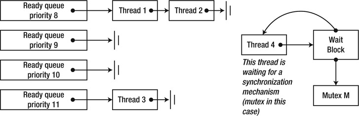
Figure 6-9 . The data maintained by the operating system scheduler. Threads ready for execution are placed in FIFO queues, sorted by priority. Blocked threads reference their synchronization mechanism through an internal structure called a wait block
Overall, there are potentially thousands of CPU cycles spent to block a thread, and a similar number of cycles is required to unblock it when the synchronization mechanism becomes available. It is clear, then, that if a kernel synchronization mechanism is used to protect a long-running operation, such as writing a large buffer to a file or performing a network round-trip, this overhead is negligible, but if a kernel synchronization mechanism is used to protect an operation like ++i, this overhead introduces an inexcusable slowdown.
The synchronization mechanisms Windows and .NET make available to applications differ primarily in terms of their acquire and release semantics, also known as their signal state. When a synchronization mechanism becomes signaled, it wakes up a thread (or a group of threads) waiting for it to become available. Below are the signal state semantics for some of the synchronization mechanisms currently accessible to .NET applications:
Table 6-1. Signal State Semantics of Some Synchronization Mechanisms
| Synchronization Mechanism | When Does It Become Signaled? | Which Threads Are Woken? |
|---|---|---|
| Mutex | When a thread calls Mutex.ReleaseMutex | One of the threads that are waiting for the mutex |
| Semaphore | When a thread calls Semaphore.Release | One of the threads that are waiting for the semaphore |
| ManualResetEvent | When a thread calls ManualResetEvent.Set | All of the threads that are waiting for the event |
| AutoResetEvent | When a thread calls AutoResetEvent.Set | One of the threads that are waiting for the event |
| Monitor | When a thread calls Monitor.Exit | One of the threads that are waiting for the Monitor |
| Barrier | When all the participating threads have called Barrier.SignalAndWait | All of the threads that are waiting for the barrier |
| ReaderWriterLock—for reading | When there are no writer threads, or the last writer thread has released the lock for writing | All of the threads that are waiting to enter the lock for reading |
| ReaderWriterLock—for writing | When there are no reader threads or writer threads | One of the threads that are waiting to enter the lock for writing |
Other than the signal state semantics, some synchronization mechanisms differ also in terms of their internal implementation. For example, the Win32 critical section and the CLR Monitor implement an optimization for locks that are currently available. With that optimization, a thread attempting to acquire an available lock can grab it directly without performing a system call. On a different front, the reader-writer lock family of synchronization mechanisms distinguishes between readers and writers accessing a certain object, which permits better scalability when the data is most often accessed for reading.
Choosing the appropriate synchronization mechanism from the list of what Windows and .NET have to offer is often difficult, and there are times when a custom synchronization mechanism may offer better performance characteristics or more convenient semantics than the existing ones. We will not consider synchronization mechanisms any further; it is your responsibility when programming concurrent applications to choose responsibly between lock-free synchronization primitives and blocking synchronization mechanisms, and to determine the best combination of synchronization mechanisms to use.
![]() Note No discussion of synchronization could be complete without highlighting data structures (collections) designed from the ground up for concurrency. Such collections are thread-safe—they allow safe access from multiple threads—as well as scalable without introducing unreasonable performance degradation due to locking. For a discussion of concurrent collections, as well as designing concurrent collections, consult Chapter 5.
Note No discussion of synchronization could be complete without highlighting data structures (collections) designed from the ground up for concurrency. Such collections are thread-safe—they allow safe access from multiple threads—as well as scalable without introducing unreasonable performance degradation due to locking. For a discussion of concurrent collections, as well as designing concurrent collections, consult Chapter 5.
We have previously paid a visit to the subject of processor caches in the context of collection implementation and memory density. In parallel programs it is similarly important to regard cache size and hit rates on a single processor, but it is even more important to consider how the caches of multiple processors interact. We will now consider a single representative example, which demonstrates the important of cache-oriented optimization, and emphasizes the value of good tools when it concerns performance optimization in general.
First, examine the following sequential method. It performs the rudimentary task of summing all the elements in a two-dimensional array of integers and returns the result.
public static int MatrixSumSequential(int[,] matrix) {
  int sum = 0;
  int rows = matrix.GetUpperBound(0);
  int cols = matrix.GetUpperBound(1);
  for (int i = 0; i < rows; ++i) {
    for (int j = 0; j < cols; ++j) {
    sum + = matrix[i,j];
    }
  }
  return sum;
}
We have in our arsenal a large set of tools for parallelizing programs of this sort. However, imagine for a moment that we don’t have the TPL at our disposal, and choose to work directly with threads instead. The following attempt at parallelization may appear sufficiently reasonable to harvest the fruits of multi-core execution, and even implements a crude aggregation to avoid synchronization on the shared sum variable:
public static int MatrixSumParallel(int[,] matrix) {
  int sum = 0;
  int rows = matrix.GetUpperBound(0);
  int cols = matrix.GetUpperBound(1);
  const int THREADS = 4;
  int chunk = rows/THREADS; //should divide evenly
  int[] localSums = new int[THREADS];
  Thread[] threads = new Thread[THREADS];
  for (int i = 0; i < THREADS; ++i) {
    int start = chunk*i;
    int end = chunk*(i + 1);
    int threadNum = i; //prevent the compiler from hoisting the variable in the lambda capture
    threads[i] = new Thread(() => {
    for (int row = start; row < end; ++row) {
    for (int col = 0; col < cols; ++col) {
    localSums[threadNum] + = matrix[row,col];
    }
    }
    });
    threads[i].Start();
  }
  foreach (Thread thread in threads) {
    thread.Join();
  }
  sum = localSums.Sum();
  return sum;
}
Executing each of the two methods 25 times on an Intel i7 processor produced the following results for a 2,000 × 2,000 matrix of integers: the sequential method completed within 325ms on average, whereas the parallelized method took a whopping 935ms on average, thrice as slow as the sequential version!
This is clearly unacceptable, but why? This is not another example of too fine-grained parallelism, because the number of threads is only 4. If you accept the premise that the problem is somehow cache-related (because this example appears in the “Cache Considerations” section), it would make sense to measure the number of cache misses introduced by the two methods. The Visual Studio profiler (when sampling at each 2,000 cache misses) reported 963 exclusive samples in the parallel version and only 659 exclusive samples in the sequential version; the vast majority of samples were on the inner loop line that reads from the matrix.
Again, why? Why would the line of code writing to the localSums array introduce so many more cache misses than the line writing to the sum local variable? The simple answer is that the writes to the shared array invalidate cache lines at other processors, causing every + = operation on the array to be a cache miss.
As you recall from Chapter 5, processor caches are organized in cache lines, and adjacent memory locations share the same cache line. When one processor writes to a memory location that is in the cache of another processor, the hardware causes a cache invalidation that marks the cache line in the other processor’s cache as invalid. Accessing an invalid cache line causes a cache miss. In our example above, it is very likely that the entire localSums array fits in a single cache line, and resides simultaneously in the caches of all four processors on which the application’s threads are executing. Every write performed to any element of the array on any of the processors invalidates the cache line on all other processors, causing a constant ping-pong of cache invalidations (see Figure 6-10).
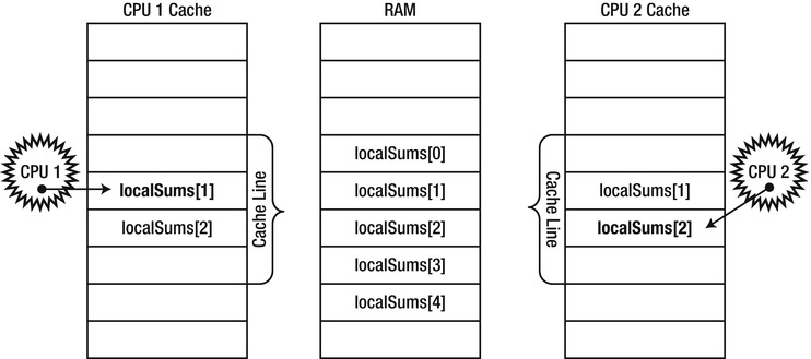
Figure 6-10 . CPU 1 writes to localSums[1] while CPU 2 writes to localSums[2]. Because both array elements are adjacent and fit into the same cache line in both processor caches, each such write causes a cache invalidation on the other processor
To make sure that the problem is completely related to cache invalidations, it is possible to make the array strides sufficiently larger such that cache invalidation does not occur, or to replace the direct writes to the array with writes to a local variable in each thread that is eventually flushed to the array when the thread completes. Either of these optimizations restores sanity to the world, and makes the parallel version faster than the sequential one on a sufficiently large number of cores.
Cache invalidation (or cache collision) is a nasty problem that is exceptionally difficult to detect in a real application, even when aided by powerful profilers. Taking it into consideration upfront when designing CPU-bound algorithms will save you a lot of time and aggravation later.
![]() Note The authors encountered a similar case of cache invalidation in a production scenario with a shared work item queue between two threads executing on two different processors. When a certain minor change was made to the internal structure of the queue class’ fields, significant performance degradation (approximately 20%) was detected in subsequent builds. Upon very long and detailed examination, it became apparent that reordering fields in the queue class was responsible for the performance degradation; two fields that were being written to by different threads have become too close together and were placed on the same cache line. Adding padding betwee the fields restored the queue’s performance to acceptable levels.
Note The authors encountered a similar case of cache invalidation in a production scenario with a shared work item queue between two threads executing on two different processors. When a certain minor change was made to the internal structure of the queue class’ fields, significant performance degradation (approximately 20%) was detected in subsequent builds. Upon very long and detailed examination, it became apparent that reordering fields in the queue class was responsible for the performance degradation; two fields that were being written to by different threads have become too close together and were placed on the same cache line. Adding padding betwee the fields restored the queue’s performance to acceptable levels.
So far, our coverage of parallel programming has been partial to CPU cores. Indeed, we have several skills at our disposal to parallelize programs across multiple cores, synchronize access to shared resources, and use high-speed CPU primitives for lock-free synchronization. As we noted at the outset of this chapter, there is another source of parallelism available to our programs—the GPU, which on modern hardware offers considerably many cores than even high-end CPUs. GPU cores are very suitable for data-parallel algorithms, and their sheer number makes up for the clumsiness often associated with running programs on them. In this section we examine one way of running programs on the GPU, using a set of C++ language extensions called C++ AMP.
![]() Note C++ AMP is based on C++, which is why this section will use C++ code examples. However, by applying a moderate amount of .NET Interoperability, you can use C++ AMP algorithms in your .NET applications as well. We will return to this subject at the end of the section.
Note C++ AMP is based on C++, which is why this section will use C++ code examples. However, by applying a moderate amount of .NET Interoperability, you can use C++ AMP algorithms in your .NET applications as well. We will return to this subject at the end of the section.
At its essence, a GPU is a processor like any other, with a specific instruction set, numerous cores, and a memory access protocol. However, there are significant differences between modern GPUs and CPUs, and understanding them is central for writing efficient GPU-based programs:
- There is only a small subset of instructions available to modern CPUs that are available on the GPU. This implies some limitations: there are no function calls, data types are limited, library functions are missing, and others. Other operations, such as branching, may introduce a performance cost unparalleled to that on the CPU. Clearly, this makes porting massive amounts of code from the CPU to the GPU a considerable effort.
- There is a considerably larger number of cores on a mid-range graphics card than on a mid-range CPU socket. There will be work units that are too small or cannot be broken into sufficiently many pieces to benefit properly from parallelization on the GPU.
- There is scarce support for synchronization between GPU cores executing a task, and no support for synchronization between GPU cores executing different tasks. This requires the synchronization and orchestration of GPU work to be performed on the CPU.
WHAT TASKS ARE SUITABLE FOR EXECUTION ON THE GPU?
Not every algorithm is suitable for execution on the GPU. For example, GPUs do not have access to other I/O devices, so you can scarcely improve the performance of a program that fetches RSS feeds from the Web by using a GPU. However, many CPU-bound data-parallel algorithms can be ported to the GPU and procure from it massive parallelization. Here are some examples (the list is by no means exhaustive):
- Image blur, sharpen, and other transformations
- Fast Fourier Transform
- Matrix transpose and multiplication
- Number sorting
- Brute-force hash reversal
A good source of additional examples is the Microsoft Native Concurrency team blog (http://blogs.msdn.com/b/nativeconcurrency/), which has sample code and explanations for a variety of algorithms that have been ported to C++ AMP.
C++ AMP is a framework that ships with Visual Studio 2012 and provides C++ developers with simple means to run computations on the GPU, and requires only a DirectX 11 driver to run. Microsoft has released C++ AMP as an open specification (available online at the time of writing at http://blogs.msdn.com/b/nativeconcurrency/archive/2012/02/03/c-amp-open-spec-published.aspx), which any compiler vendor can implement. In C++ AMP, code can execute on accelerators, which represent computational devices. C++ AMP discovers dynamically all the accelerators with a DirectX 11 driver. Out of the box, C++ AMP also ships with a reference accelerator that performs software emulation, and a CPU-based accelerator, WARP, which is a reasonable fallback on machines without a GPU or with a GPU that doesn’t have a DirectX 11 driver, and uses multi-core and SIMD instructions.
With no further ado, let us consider an algorithm that can be easily parallelized on the GPU. The algorithm below takes two vectors of the same length and calculates a pointwise result. There’s hardly anything that could be more straightforward:
void VectorAddExpPointwise(float* first, float* second, float* result, int length) {
  for (int i = 0; i < length; ++i) {
    result[i] = first[i] + exp(second[i]);
  }
}
Parallelizing this algorithm on the CPU requires splitting the iteration range into several chunks and creating a thread to handle each part. Indeed, we have devoted quite some time to doing just that with our primality testing example—we have seen how to parallelize it by manually creating threads, by issuing work items to the thread pool, and by using the Parallel.For automatic parallelization capabilities. Also, recall that when parallelizing similar algorithms on the CPU we have taken great care to avoid work items that were too granular (e.g., a work item per iteration wouldn’t do).
On the GPU, no such caution is necessary. The GPU is equipped with many cores that can execute threads very rapidly, and the cost of a context switch is significantly lower than on the CPU. Below is the code required using C++ AMP’s parallel_foreach API:
#include < amp.h>
#include < amp_math.h>
using namespace concurrency;
void VectorAddExpPointwise(float* first, float* second, float* result, int length) {
  array_view < const float,1 > avFirst (length, first);
  array_view < const float,1 > avSecond(length, second);
  array_view < float,1> avResult(length, result);
  avResult.discard_data();
  parallel_for_each(avResult.extent, [=](index < 1 > i) restrict(amp) {
    avResult[i] = avFirst[i] + fast_math::exp(avSecond[i]);
  });
  avResult.synchronize();
}
We now examine each part of the code individually. First, the general shape of the main loop has been maintained, although the original for loop has been replaced with an API call to parallel_foreach. Indeed, the principle of converting a loop to an API call is not new—we have seen the same with TPL’s Parallel.For and Parallel.ForEach APIs.
Next, the original data passed to the method (the first, second, and result parameters) has been wrapped in array_view instances. The array_view class wraps data that must be moved to an accelerator (GPU). Its template parameters are the type of the data and its dimensionality. If we want the GPU to execute instructions that access data that was originally on the CPU, some entity must take care of copying the data to the GPU, because most of today’s GPUs are discrete devices with their own memory. This is the task of the array_view instances—they make sure data is copied on demand, and only when it is required.
When the work on the GPU is done, the data is copied back to its original location. By creating array_view instances with a const template type argument, we make sure that first and second are copied only to the GPU but don’t have to be copied back from the GPU. Similarly, by calling the discard_data method, we make sure that result is not copied from the CPU to the GPU, but only from the GPU to the CPU when there is a result worth copying.
The parallel_foreach API takes an extent, which is the shape of the data we are working on, and a function to execute for each of the elements in the extent. We used a lambda function in the code above, which is a welcome addition to C++ as of the 2011 ISO C++ standard (C++11). The restrict(amp) keyword instructs the compiler to verify that the body of the function can execute on the GPU, forbidding most of the C++ syntax—syntax that cannot be compiled to GPU instructions.
The lambda function’s parameter is an index < 1 > object, which represents a one-dimensional index. This must match the extent we used—should we declare a two-dimensional extent (such as the data shape of a matrix), the index would have to be two-dimensional as well. We will see an example of this shortly.
Finally, the synchronize method call at the end of the method makes sure that by the time VectorAdd returns, the changes made on the CPU to the avResult array_view are copied back into its original container, the result array.
This concludes our first foray into the world of C++ AMP, and we are ready for a closer examination of what is going on—as well as a better example, which will yield benefits from GPU parallelization. Vector addition is not the most exciting of algorithms, and does not make a good candidate for offloading to the GPU because the memory transfer outweights the computation’s parallelization. In the following subsection we look at two examples that should be more interesting.
The first “real-world” example we shall consider is matrix multiplication. We will optimize the naïve cubic time algorithm for matrix multiplication and not Strassen’s algorithm, which runs in sub-cubic time. Given two matrices of suitable dimensions, A that is m-by-w and B that is w-by-n, the following sequential program produces their product, a matrix C that is m-by-n:
void MatrixMultiply(int* A, int m, int w, int* B, int n, int* C) {
  for (int i = 0; i < m; ++i) {
    for (int j = 0; j < n; ++j) {
    int sum = 0;
    for (int k = 0; k < w; ++k) {
    sum + = A[i*w + k] * B[k*w + j];
    }
    C[i*n + j] = sum;
    }
  }
}
There are several sources for parallelism here, and if you were willing to parallelize this code on the CPU, you might be right in suggesting that we parallelize the outer loop and be done with it. On the GPU, however, there are sufficiently many cores that if we parallelize only the outer loop we might not create enough work for all the cores. Therefore, it makes sense to parallelize the two outer loops, still leaving a meaty algorithm for the inner loop:
void MatrixMultiply(int* A, int m, int w, int* B, int n, int* C) {
  array_view < const int,2 > avA(m, w, A);
  array_view < const int,2 > avB(w, n, B);
  array_view < int,2> avC(m, n, C);
  avC.discard_data();
  parallel_for_each(avC.extent, [=](index < 2 > idx) restrict(amp) {
    int sum = 0;
    for (int k = 0; k < w; ++k) {
    sum + = avA(idx[0]*w, k) * avB(k*w, idx[1]);
    }
    avC[idx] = sum;
  });
}
Everything is still very similar to sequential multiplication and the vector addition example we have seen earlier—with the exception of the index, which is two-dimensional, and accessed by the inner loop using the [] operator. How does this version fare compared to the sequential CPU alternative? To multiply two 1024 × 1024 matrices (of integers), the CPU version required 7350 ms on average, whereas the GPU version—hold tight—took 50 ms on average, a 147-fold improvement!
The examples we have seen so far had very trivial code in the inner loop that was scheduled on the GPU. Clearly, this must not always be the case. One of the examples on the Native Concurrency team blog we referred to demonstrates an N-body simulation, which simulates the interactions between particles where the force of gravity is applied. The simulation consists of an infinite number of steps; in each step, it has to determine the updated acceleration vector of each particle and then determine its new location. The parallelizable component here is the vector of particles—with sufficiently many particles (a few thousands or more) there is ample work for all GPU cores to do at once.
The kernel that determines the result of an interaction between two bodies is the following code, which can be ported very easily to the GPU:
//float4 here is a four-component vector with pointwise operations
void bodybody_interaction(
  float4& acceleration, const float4 p1, const float4 p2) restrict(amp) {
  float4 dist = p2 – p1;
  float absDist = dist.x*dist.x + dist.y*dist.y + dist.z*dist.z; //w is unused here
  float invDist = 1.0f / sqrt(absDist);
  float invDistCube = invDist*invDist*invDist;
  acceleration + = dist*PARTICLE_MASS*invDistCube;
}
Each simulation step takes an array of particle positions and velocities, and generates a new array of particle positions and velocities based on the results of the simulation:
struct particle {
  float4 position, velocity;
  //ctor, copy ctor, and operator = with restrict(amp) omitted for brevity
};
void simulation_step(array < particle,1 > & previous, array < particle,1 > & next, int bodies) {
  extent < 1 > ext(bodies);
  parallel_for_each(ext, [&](index < 1 > idx) restrict(amp) {
    particle p = previous[idx];
    float4 acceleration(0, 0, 0, 0);
    for (int body = 0; body < bodies; ++body) {
    bodybody_interaction(acceleration, p.position, previous[body].position);
    }
    p.velocity + = acceleration*DELTA_TIME;
    p.position + = p.velocity*DELTA_TIME;
    next[idx] = p;
  });
}
With an appropriate GUI, this simulation is very entertaining. The full sample provided by the C++ AMP team is available on the Native Concurrency blog. On the author’s system, an Intel i7 processor with an ATI Radeon HD 5800 graphics card, a simulation with 10,000 particles yielded ∼ 2.5 frames per second (steps) from the sequential CPU version and 160 frames per second (steps) from the optimized GPU version (see Figure 6-11), an incredible improvement.
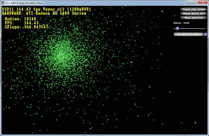
Figure 6-11 . N-body simulation UI demo, showing >160 frames per second (simulation steps) when using the optimized C++ AMP implementation with 10,240 simulated particles
Before we conclude this section, there is a very important optimization surfaced by C++ AMP that can improve even more the performance of our GPU code. GPUs offer a programmable data cache (often called shared memory). Values stored in it are shared across all threads in the same tile. By using tiled memory, C++ AMP programs can read data from the GPU’s main memory once into the shared tile memory, and then access it quickly from multiple threads in the same tile without refetching it from the GPU’s main memory. Accessing shared tile memory can be around 10 times faster than accessing the GPU’s main memory—in other words, you have a reason to keep reading.
To execute a tiled version of a parallel loop, the parallel_for_each method accepts a tiled_extent domain, which subdivides a multi-dimensional extent into multi-dimensional tiles, and a tiled_index lambda parameter, which specifies both the global thread ID within the extent, and the local thread ID within the tile. For example, a 16 × 16 matrix can be subdivided into 2 × 2 tiles (see Figure 6-12) and then passed into parallel_for_each:
extent < 2 > matrix(16,16);
tiled_extent < 2,2 > tiledMatrix = matrix.tile < 2,2 > ();
parallel_for_each(tiledMatrix, [=](tiled_index < 2,2 > idx) restrict(amp) { . . . });
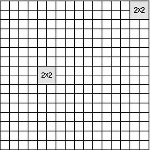
Figure 6-12 . A 16 × 16 matrix is divided into tiles of 2 × 2 each. Every four threads that belong in the same tile can share data between them
Within the GPU kernel, idx.global can be used in place of the standard index < 2 > we have seen earlier when performing operations on matrices. However, clever use of the local tile memory and local tile indices can reap significant performance benefits. To declare tile-specific memory that is shared across all threads in the same tile, the tile_static storage specifier can be applied to local variables inside the kernel. It is common to declare a shared memory location and have each thread in the tile initialize a small part of it:
parallel_for_each(tiledMatrix, [=](tiled_index < 2,2 > idx) restrict(amp) {
  tile_static int local[2][2]; //32 bytes shared between all threads in the tile
  local[idx.local[0]][idx.local[1]] = 42; //assign to this thread's location in the array
});
Clearly, procuring any benefits from memory shared with other threads in the same tile is only possible if all the threads can synchronize their access to the shared memory; i.e., they shouldn’t attempt to access shared memory locations before their tile neighboring threads have initialized them. tile_barrier objects synchronize the execution of all the threads in a tile—they can proceed executing after calling tile_barrier.wait only after all the threads in the tile have called tile_barrier.wait as well (this is similar to the TPL’s Barrier class). For example:
parallel_for_each(tiledMatrix, [](tiled_index < 2,2 > idx) restrict(amp) {
  tile_static int local[2][2]; //32 bytes shared between all threads in the tile
  local[idx.local[0]][idx.local[1]] = 42; //assign to this thread's location in the array
  idx.barrier.wait(); //idx.barrier is a tile_barrier instance
  //Now this thread can access "local" at other threads' indices!
});
It is now time to apply all this knowledge to a concrete example. We will revisit the matrix multiplication algorithm previously implemented without tiling, and introduce a tiling-based optimization into it. Let’s assume that the matrix dimensions are divisible by 256—this allows us to work with 16 × 16 thread tiles. Matrix multiplication contains inherent blocking, which can be used to our advantage (in fact, one of the most common optimizations of extremely large matrix multiplication on the CPU is by using blocking to obtain better cache behavior). The primary observation boils down to the following. To find C i,j (the element at row i and column j in the result matrix), we have to find the scalar product between A i,* (the entire i-th row of the first matrix) and B *,j (the entire j-th row of the second matrix). However, this is equivalent to finding the scalar products of partial rows and partial columns and summing the results together. We can use this to translate our matrix multiplication algorithm to the tiled version:
void MatrixMultiply(int* A, int m, int w, int* B, int n, int* C) {
  array_view < const int,2 > avA(m, w, A);
  array_view < const int,2 > avB(w, n, B);
  array_view < int,2> avC(m, n, C);
  avC.discard_data();
  parallel_for_each(avC.extent.tile < 16,16 > (), [=](tiled_index < 16,16 > idx) restrict(amp) {
    int sum = 0;
    int localRow = idx.local[0], localCol = idx.local[1];
    for (int k = 0; k < w; k += 16) {
    tile_static int localA[16][16], localB[16][16];
    localA[localRow][localCol] = avA(idx.global[0], localCol + k);
    localB[localRow][localCol] = avB(localRow + k, idx.global[1]);
    idx.barrier.wait();
    for (int t = 0; t < 16; ++t) {
    sum + = localA[localRow][t]*localB[t][localCol];
    }
    idx.barrier.wait(); //to avoid having the next iteration overwrite the shared memory
    }
    avC[idx.global] = sum;
  });
}
The essence of the tiled optimization is that each thread in the tile (there are 256 threads, the tile is 16 × 16) initializes its own element in the 16 × 16 local copies of sub-blocks from the A and B input matrices (see Figure 6-13). Each thread in the tile needs only one row and one column of these sub-blocks, but all the threads together will access every row 16 times and every column 16 times, reducing significantly the number of main memory accesses.
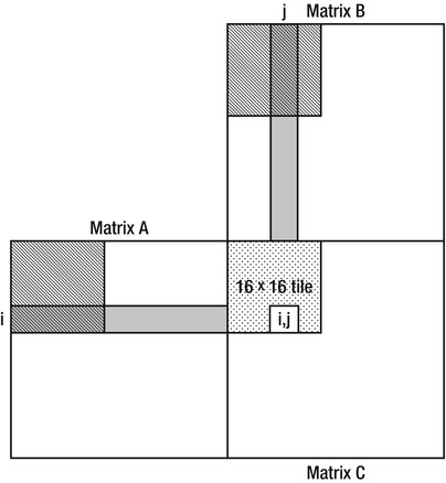
Figure 6-13 . To find the element (i,j) in the result matrix, the algorithm requires the entire i-th row of the first matrix and j-th column of the second matrix. When the threads in the 16 × 16 tile shown in the diagram execute and k = 0, the shaded areas in the first and second matrices will eventually be read into shared memory. The thread responsible for the (i,j)-th element in the result matrix will then have the partial scalar product of the first k elements from the i-th row with the first k elements from the j-th row
In this case, tiling is a worthwhile optimization. The tiled version of matrix multiplication executes significantly faster than the simple one, and takes 17 ms on average to complete (using the same 1024 × 1024 matrices). This concludes a 430-fold speed increase compared to the CPU version!
Before we part with C++ AMP, it’s worthwhile to mention the development tools (Visual Studio) available to C++ AMP developers. Visual Studio 2012 features a GPU debugger, which you can use to place breakpoints in GPU kernels, inspect simulated call stacks, read and modify local variables (some accelerators support GPU debugging; with others, Visual Studio uses a software emulator), and a profiler that can be used to gauge what your application has gained from using GPU parallelization. For more information on the Visual Studio GPU debugging experience, consult the MSDN article “Walkthrough: Debugging a C++ AMP Application”, at http://msdn.microsoft.com/en-us/library/hh368280(v=VS.110).aspx.
.NET ALTERNAT IVES FOR GPGPU COMPUTING
Although so far this entire section has dealt exclusively with C++, there are several options for harnessing the power of the GPU from managed applications. One option is to use managed-native interoperability (discussed in Chapter 8), deferring to a native C++ component to implement the GPU kernels. This is a reasonable option if you like C++ AMP, or have a reusable C++ AMP component that is used in managed applications as well as native ones.
Another option is to use a library that works with the GPU directly from managed code. There are several such libraries available, for example GPU.NET and CUDAfy.NET (both commercial offerings). Here is an example from GPU.NET GitHub repository, demonstrating a scalar product of two vectors:
[Kernel]
public static void MultiplyAddGpu(double[] a, double[] b, double[] c) {
 int ThreadId = BlockDimension.X * BlockIndex.X + ThreadIndex.X;
 int TotalThreads = BlockDimension.X * GridDimension.X;
 for (int ElementIdx = ThreadId; ElementIdx < a.Length; ElementIdx += TotalThreads) {
 c[ElementIdx] = a[ElementIdx] * b[ElementIdx];
}
}
In the authors’ opinion, language extensions (the C++ AMP approach) are more effective and easier to learn than attempts to bridge the gap purely at the library level, or by introducing significant IL rewriting.
This section hardly scratches the surface of the possibilities offered by C++ AMP. We have only taken a look at some of the APIs and parallelized an algorithm or two. If you are interested in more details about C++ AMP, we strongly recommend Kate Gregory’s and Ade Miller’s book, “C++ AMP: Accelerated Massive Parallelism with Microsoft Visual C++” (Microsoft Press, 2012).
Summary
Through the course of this chapter, it has become evident that parallelization is a crucial tool to have for performance optimization work. On many servers and workstations around the world, CPUs and GPUs idle and waste precious hardware resources because applications fail to tap into the machine’s full computing power. With the Task Parallel Library at our disposal, taking advantage of all available CPU cores is easier than before, although synchronization problems, oversubscription, and unequal work distribution leave some interesting issues and pitfalls to deal with. On the GPU front, C++ AMP and other libraries for general-purpose GPU computing are flourishing with algorithms and APIs to parallelize your code on hundreds of GPU cores. Finally, unexploited in this chapter, remain the performance gains harvestable from distributed computing—the cloud—which is the biggest trend in IT today.