
![]()
Smart Scans and Offloading
One of the enhancements provided by Exadata is the Smart Scan, a mechanism by which parts of a query can be offloaded, or handed off, to the storage servers for processing. This “divide-and-conquer” approach is one reason Exadata is able to provide such stellar performance. It’s accomplished by the configuration of Exadata, where database servers and storage cells offer computing power and the ability to process queries, owing to the unique storage server software running on the storage cells.
Smart Scans
Not every query qualifies for a Smart Scan, as certain conditions must be met. Those conditions are as follows:
- A full table scan or full index scan must be used, in addition to direct-path reads.
- One or more of the following simple comparison operators must be in use:
- =
- <
- >
- >=
- =<
- BETWEEN
- IN
- IS NULL
- IS NOT NULL
Smart Scans will also be available when queries are run in parallel, because direct-path reads are executed by default, by parallel query slaves. Of course, the other conditions must also be met: parallel only ensures that direct-path reads are used. What does a Smart Scan do to improve performance? It reduces the amount of data the database servers must process to return results. The offloading process divides the workload among the compute nodes and the storage cells, involves more CPU resources, and returns smaller sets of data to the receiving process.
Instead of reading 10,000 blocks of data to return 1,000 rows, offloading allows the storage cells to perform some of the work with access and filter predicates and to send back only the rows that meet the provided criteria. Similar in operation to parallel query slaves, the offloading process divides the work among the available storage cells, and each cell returns any qualifying rows stored in that particular subset of disks. And, like parallel query, the result “pieces” are merged into the final result set. Offloading also reduces inter-instance transfer between nodes, which, in turn, reduces latching and global locking. Latching, in particular, consumes CPU cycles. Less latching equates to a further reduction in CPU cycles, enhancing performance. The net “savings” in CPU work and execution time can be substantial; queries that take minutes to execute on non-Exadata systems can sometimes be completed in seconds as a result of using Smart Scans.
Plans and Metrics
Execution plans can report Smart Scan activity, if they are the actual plans generated by the optimizer at runtime. Qualifying plans will be found in the V$SQL_PLAN and DBA_HIST_SQL_PLAN views and will be generated by autotrace, when the ON option is used, or can be found by enabling a 10046 trace and processing the resulting trace file through tkprof. Using autotrace in EXPLAIN mode may not provide the same plan as generated at runtime, because it can still use rule-based optimizer decisions to generate plans. The same holds true for EXPLAIN PLAN. (We have seen cases where EXPLAIN PLAN and a 10046 trace differed in the reported execution plan.) The tkprof utility also offers an explain mode, and it, too, can provide misleading plans. By default, tkprof provides the actual plan from the execution, so using the command-line explain option is unnecessary.
Smart Scans are noted in the execution plan in one of three ways:
- TABLE ACCESS STORAGE FULL
- INDEX STORAGE FULL SCAN
- INDEX STORAGE FAST FULL SCAN
The presence of one or more of these operations does not mean that a Smart Scan actually occurred; other metrics should be used to verify Smart Scan execution. The V$SQL view (and, for RAC databases, GV$SQL) has two columns that provide further information on cell offload execution, io_cell_offload_eligible_bytes and io_cell_offload_returned_bytes. These are populated with relevant information regarding cell offload activity for a given sql_id, provided a Smart Scan was actually executed.
The io_cell_offload_eligible_bytes column reports the bytes of data that qualify for offload. This is the volume of data that can be offloaded to the storage cells during query execution. The io_cell_offload_returned_bytes column reports the number of bytes returned by the regular I/O path. These are the bytes that were not offloaded to the cells. The difference between these two values provides the bytes actually offloaded during query execution. If no Smart Scan were used, the values for both columns would be 0. There will be cases where the column io_cell_offload_eligible_bytes will be equal to 0, but the column io_cell_offload_returned_bytes will not. Such cases will usually, but not always, be referencing either fixed views (such as GV$SESSION_WAIT) or other data dictionary views (V$TEMPSEG_USAGE, for example). Such queries are not considered eligible for offload. (The view isn’t offloadable, because it may expose memory structures resident on the database compute nodes, but that doesn’t indicate they don’t qualify for a Smart Scan [one or more of the base tables to that view might qualify].) The presence of projection data in V$SQL_PLAN/GV$SQL_PLAN is proof enough that a Smart Scan was executed.
Looking at a query where a Smart Scan is executed, using the smart_scan_ex.sql script, we see
SQL> select *
  2  from emp
  3  where empid = 7934;

     EMPID EMPNAME                                      DEPTNO
---------- ---------------------------------------- ----------
      7934 Smorthorper7934                                  15

Elapsed: 00:00:00.21

Execution Plan
----------------------------------------------------------
Plan hash value: 3956160932

----------------------------------------------------------------------------------
| Id  | Operation                 | Name | Rows  | Bytes | Cost (%CPU)| Time     |
----------------------------------------------------------------------------------
|   0 | SELECT STATEMENT          |      |     1 |    28 |  6361   (1)| 00:00:01 |
|*  1 |  TABLE ACCESS STORAGE FULL| EMP  |     1 |    28 |  6361   (1)| 00:00:01 |
----------------------------------------------------------------------------------

Predicate Information (identified by operation id):
---------------------------------------------------

   1 - storage("EMPID"=7934)
       filter("EMPID"=7934)

Statistics
----------------------------------------------------------
    1  recursive calls
    1  db block gets
40185  consistent gets
22594  physical reads
  168  redo size
  680  bytes sent via SQL*Net to client
  524  bytes received via SQL*Net from client
    2  SQL*Net roundtrips to/from client
    0  sorts (memory)
    0  sorts (disk)
    1  rows processed

SQL>
Notice that the execution plan reports, via the TABLE ACCESS STORAGE FULL operation, that a Smart Scan is in use. Verifying that with a quick query to V$SQL we see
     SQL>select  sql_id,
  2  io_cell_offload_eligible_bytes qualifying,
  3  io_cell_offload_eligible_bytes - io_cell_offload_returned_bytes actual,
  4  round(((io_cell_offload_eligible_bytes - io_cell_offload_returned_bytes)/io_cell_offload_eligible_bytes)*100, 2) io_saved_pct,
  5  sql_text
  6  from v$sql
  7  where io_cell_offload_returned_bytes> 0
  8  and instr(sql_text, 'emp') > 0
  9  and parsing_schema_name = 'BING';

SQL_ID        QUALIFYING     ACTUAL IO_SAVED_PCT SQL_TEXT
------------- ---------- ---------- ------------ -------------------------------------
gfjb8dpxvpuv6  185081856   42510928        22.97 select * from emp where empid = 7934

SQL>
The savings in I/O, as a percentage of the total eligible bytes, was 22.97 percent, meaning Oracle processed almost 23 percent less data than it would have had a Smart Scan not been executed. Setting cell_offload_processing=false in the session, the query is executed again, using the no_smart_scan_ex.sql script, as follows:
SQL> alter session set cell_offload_processing=false;

Session altered.

Elapsed: 00:00:00.00
SQL>
SQL> select *
  2  from emp
  3  where empid = 7934;

     EMPID EMPNAME                                      DEPTNO
---------- ---------------------------------------- ----------
      7934 Smorthorper7934                                  15

Elapsed: 00:00:03.73

Execution Plan
----------------------------------------------------------
Plan hash value: 3956160932

----------------------------------------------------------------------------------
| Id  | Operation                 | Name | Rows  | Bytes | Cost (%CPU)| Time     |
----------------------------------------------------------------------------------
|   0 | SELECT STATEMENT          |      |     1 |    28 |  6361   (1)| 00:00:01 |
|*  1 |  TABLE ACCESS STORAGE FULL| EMP  |     1 |    28 |  6361   (1)| 00:00:01 |
----------------------------------------------------------------------------------

Predicate Information (identified by operation id):
---------------------------------------------------

   1 - filter("EMPID"=7934)


Statistics
----------------------------------------------------------
          1  recursive calls
          1  db block gets
      45227  consistent gets
      22593  physical reads
          0  redo size
        680  bytes sent via SQL*Net to client
        524  bytes received via SQL*Net from client
          2  SQL*Net roundtrips to/from client
          0  sorts (memory)
          0  sorts (disk)
          1  rows processed

SQL>
SQL> set autotrace off timing off
SQL>
SQL> select sql_id,
  2  io_cell_offload_eligible_bytes qualifying,
  3  io_cell_offload_eligible_bytes - io_cell_offload_returned_bytes actual,
  4  round(((io_cell_offload_eligible_bytes - io_cell_offload_returned_bytes)/io_cell_offload_eligible_bytes)*100, 2) io_saved_pct,
  5  sql_text
  6  from v$sql
  7  where io_cell_offload_returned_bytes > 0
  8  and instr(sql_text, 'emp') > 0
  9  and parsing_schema_name = 'BING';

no rows selected

SQL>
In the absence of a Smart Scan, the query executed in 3.73 seconds and processed the entire 185081856 bytes of data. Because offload processing was disabled, the storage cells provided no assistance with the query processing. It is interesting to note that the execution plan reports TABLE ACCESS STORAGE FULL, a step usually associated with a Smart Scan. The absence of predicate information and the “no rows selected” result for the offload bytes query prove that a Smart Scan was not executed. Disabling cell offload processing created a noticeable difference in execution time, proving the power of a Smart Scan.
Smart Scan performance can also outshine the performance provided by an index for larger volumes of data by allowing Oracle to reduce the I/O by gigabytes, or even terabytes, of data when returning rows satisfying the query criteria. There are also cases where a Smart Scan is not the best performer; an index is added to the table and the same set of queries is executed a third time, again using the smart_scan_ex.sql script:
SQL> create index empid_idx on emp(empid);

Index created.

SQL>
SQL> set autotrace on timing on
SQL>
SQL> select *
  2  from emp
  3  where empid = 7934;

     EMPID EMPNAME                                      DEPTNO
---------- ---------------------------------------- ----------
      7934 Smorthorper7934                                  15

Elapsed: 00:00:00.01

Execution Plan
----------------------------------------------------------
Plan hash value: 1109982043

--------------------------------------------------------------------------------------
| Id | Operation                   | Name      | Rows  | Bytes | Cost(%CPU)| Time    |
--------------------------------------------------------------------------------------
|  0 | SELECT STATEMENT            |           |     1 |    28 |     4  (0)| 00:00:01|
|  1 |  TABLE ACCESS BY INDEX ROWID| EMP       |     1 |    28 |     4  (0)| 00:00:01|
|* 2 |   INDEX RANGE SCAN          | EMPID_IDX |     1 |       |     3  (0)| 00:00:01|
--------------------------------------------------------------------------------------

Predicate Information (identified by operation id):
---------------------------------------------------

   2 - access("EMPID"=7934)


Statistics
----------------------------------------------------------
  1  recursive calls
  0  db block gets
  5  consistent gets
  2  physical reads
148  redo size
684  bytes sent via SQL*Net to client
524  bytes received via SQL*Net from client
  2  SQL*Net roundtrips to/from client
  0  sorts (memory)
  0  sorts (disk)
  1  rows processed
SQL>
SQL> set autotrace off timing off
SQL>
SQL>select sql_id,
  2  io_cell_offload_eligible_bytes qualifying,
  3  io_cell_offload_returned_bytes actual,
  4  round(((io_cell_offload_eligible_bytes - io_cell_offload_returned_bytes)/io_cell_offload_eligible_bytes)*100, 2) io_saved_pct,
  5  sql_text
  6  from v$sql
  7  where io_cell_offload_returned_bytes> 0
  8  and instr(sql_text, 'emp') > 0
  9  and parsing_schema_name = 'BING';

no rows selected

SQL>
Notice that an index range scan was chosen by the optimizer, rather than offloading the predicates to the storage cells. The elapsed time for the index-range scan was considerably less than the elapsed time for the Smart Scan, so, in some cases, a Smart Scan may not be the most efficient path to the data. This also illustrates an issue with existing indexes, as the optimizer may select an index that makes the execution path worse, which explains why some Exadata sources recommend dropping indexes to improve performance. Although it may eventually be decided that dropping an index is best for the overall performance of a query or group of queries, no such recommendation is offered here, as each situation is different and needs to be evaluated on a case-by-case basis; what’s good for one Exadata system and application may not be good for another. The only way to know, with any level of certainty, whether or not to drop a particular index is to test and evaluate the results in an environment as close to production as possible.
Smart Scan Optimizations
A Smart Scan uses various optimizations to accomplish its task. There are three major optimizations a Smart Scan implements: Column Projection, Predicate Filtering, and storage indexes. Because storage indexes will be covered in detail in the next chapter, this discussion will concentrate on the first two optimizations. Suffice it to say, for now, that storage indexes are not like conventional indexes, in that they inform Exadata where not to look for data. That may be confusing at this point, but it will be covered in depth later. The primary focus of the next sections will be Column Projection and Predicate Filtering.
Column Projection
What is Column Projection? It’s Exadata’s ability to return only the columns requested by the query. In conventional systems using commodity hardware, Oracle will fetch the data blocks of interest in their entirety from the storage cells, loading them into the buffer cache. Oracle then extracts the columns from these blocks, filtering them at the end to return only the columns in the select list. Thus, the entire rows of data are returned to be further processed before displaying the final results. Column Projection does the filtering before it gets to the database server, returning only columns in the select list and, if applicable, those columns necessary for join operations. Rather than return the entire data block or row, Exadata returns only what it needs to complete the query operation. This can considerably reduce the data processed by the database servers.
Take, as an example, a table with 45 columns and a select list that contains 7 of those columns. Column Projection will return only those 7 columns, rather than the entire 45, reducing the database server workload appreciably. Let’s add a two-column join condition to the query and another two columns from another table with 71 columns; Column Projection will return the nine columns from the select list and the four columns in the join condition (presuming the join columns are not in the select list). Thirteen columns are much less data than 116 columns (the 45 from the first table and the 71 from the second), which is one reason Smart Scans can be so fast. Column Projection information is available from either the PROJECTION column from V$SQL_PLAN or from the DBMS_XPLAN package, so you can choose which of the two is easier for you to use; the projection information is returned only if the “+projection” parameter is passed to the DISPLAY_CURSOR function, as was done in this example (again from smart_scan_ex.sql), which makes use of both methods of retrieving the Column Projection data:
SQL> select *
  2  from emp
  3  where empid = 7934;

     EMPID EMPNAME                                      DEPTNO
---------- ---------------------------------------- ----------
      7934 Smorthorper7934                                  15

Elapsed: 00:00:00.16

SQL> select sql_id,
  2         projection
  3  from v$sql_plan
  4  where sql_id = 'gfjb8dpxvpuv6';

SQL_ID        PROJECTION
------------- ----------------------------------------------------------------------------
gfjb8dpxvpuv6 "EMPID"[NUMBER,22], "EMP"."EMPNAME"[VARCHAR2,40], "EMP"."DEPTNO"[NUMBER,22]


SQL>
SQL> select *
  2  from table(dbms_xplan.display_cursor('&sql_id','&child_no', '+projection'));
Enter value for sql_id: gfjb8dpxvpuv6
Enter value for child_no:

PLAN_TABLE_OUTPUT
-------------------------------------------------------------------------------------------SQL_ID  gfjb8dpxvpuv6, child number 0
-------------------------------------
select * from emp where empid = 7934

Plan hash value: 3956160932


----------------------------------------------------------------------------------
| Id  | Operation                 | Name | Rows  | Bytes | Cost (%CPU)| Time     |
----------------------------------------------------------------------------------
|   0 | SELECT STATEMENT          |      |       |       |  6361 (100)|          |
|*  1 |  TABLE ACCESS STORAGE FULL| EMP  |     1 |    28 |  6361   (1)| 00:00:01 |
----------------------------------------------------------------------------------

Predicate Information (identified by operation id):
---------------------------------------------------

   1 - storage("EMPID"=7934)
       filter("EMPID"=7934)

Column Projection Information (identified by operation id):
-----------------------------------------------------------

1 - "EMPID"[NUMBER,22], "EMP"."EMPNAME"[VARCHAR2,40],
    "EMP"."DEPTNO"[NUMBER,22]


29 rows selected.

SQL>
As only three columns were requested, only those three columns were returned by the storage servers (proven by the Column Projection Information section of the autotrace report), making the query execution much more efficient. The database servers had no need to filter the result set rows to return only the desired columns.
Predicate Filtering
Where Column Projection returns only the columns of interest from a select list or join condition, Predicate Filtering is the mechanism used by Exadata to return only the rows of interest. Such filtering occurs at the storage cells, which reduces the volume of data the database servers must process. The predicate information is passed on to the storage servers during the course of Smart Scan execution, so performing the filtering operation at the storage server level is a logical choice. Because the data volume to the database servers is reduced, so is the load on the database server CPUs. The preceding example used both Column Projection and Predicate Filtering to rapidly return the result set; using both is a powerful combination not available from systems configured from individual, unmatched components.
Basic Joins
Depending on the query, join processing can also be offloaded to the storage servers, and these are processed using an interesting construct known as a bloom filter . These are not new, nor are they exclusive to Exadata, as Oracle has used them in query processing since Oracle Database Version 10g Release 2, primarily to reduce traffic between parallel query slaves. What is a bloom filter? Named after Burton Howard Bloom, who came up with the concept in the 1970s, it’s an efficient data structure used to quickly determine if an element has a high probability of being a member of a given set. It’s based on a bit array that allows for rapid searches and returns one of two results: either the element is probably in the set (which can produce false positives) or the element is definitely not in the set. The filter cannot produce false negatives, and the incidence of false positives is relatively rare. Another advantage to bloom filters is their small size relative to other data structures used for similar purposes (self-balancing binary search trees, hash tables, or linked lists). The possibility of false positives necessitates the addition of another filter to eliminate them from the results, yet such a filter doesn’t add appreciably to the process time and, therefore, goes relatively unnoticed.
When bloom filters are used for a query on an Exadata system, the filter predicate and the storage predicate will list the SYS_OP_BLOOM_FILTER function as being called. This function includes the additional filter to eliminate any false positives that could be returned. It’s the storage predicate that provides the real power of the bloom filter on Exadata. Using a bloom filter to pre-join the tables at the storage server level reduces the volume of data the database servers need to process and can significantly reduce the execution time of the given query.
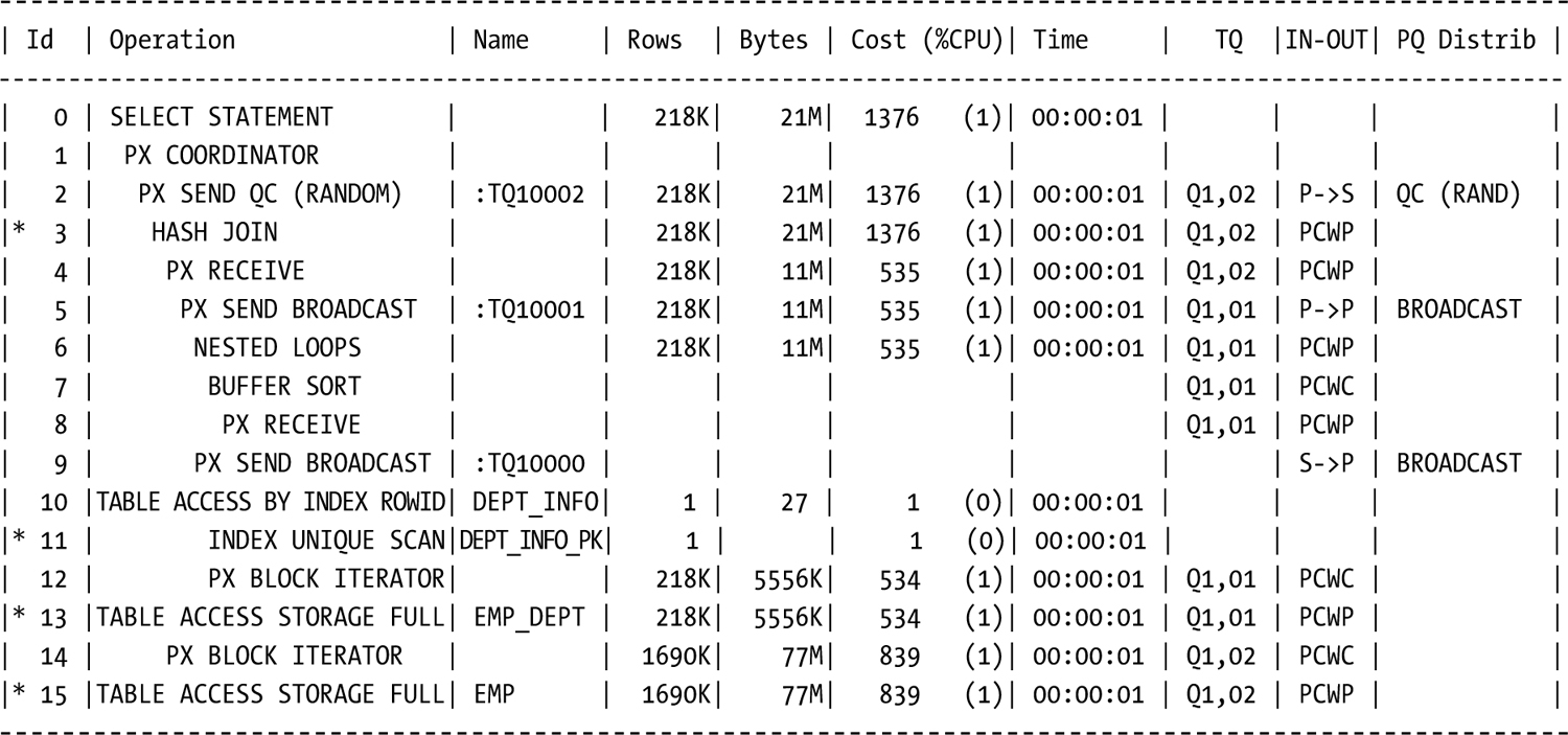
An example of bloom filters in action follows; the bloom_fltr_ex.sql script was executed to generate this output.
SQL> --
SQL> -- Create sample tables
SQL> --
SQL> -- Create them parallel, necessary
SQL> -- to get a Smart Scan on these tables
SQL> --
SQL> create table emp(
  2     empid   number,
  3     empnmvarchar2(40),
  4     empsal  number,
  5     empssn  varchar2(12),
  6     constraint emp_pk primary key (empid)
  7  ) parallel 4;

Table created.

SQL>
SQL> create table emp_dept(
  2     empid   number,
  3     empdept number,
  4     emploc  varchar2(60),
  5    constraint emp_dept_pk primary key(empid)
  6  ) parallel 4;

Table created.

SQL>
SQL> create table dept_info(
  2     deptnum number,
  3     deptnm  varchar2(25),
  4    constraint dept_info_pk primary key(deptnum)
  5  ) parallel 4;

Table created.
SQL>
SQL> --
SQL> -- Load sample tables with data
SQL> --
SQL> begin
  2          for i in 1..2000000 loop
  3                  insert into emp
  4                  values(i, 'Fnarm'||i, (mod(i, 7)+1)*1000, mod(i,10)||mod(i,10)||mod(i,10)||'-'||mod(i,10)||mod(i,10)||'-'||mod(i,10)||mod(i,10)||mod(i,10)||mod(i,10));
  5                  insert into emp_dept
  6             values(i, (mod(i,8)+1)*10, 'Zanzwalla'||(mod(i,8)+1)*10);
  7                   commit;
  8          end loop;
  9          insert into dept_info
 10          select distinct empdept, case when empdept = 10 then 'SALES'
 11                                         when empdept = 20 then 'PROCUREMENT'
 12                                         when empdept = 30 then 'HR'
 13                                         when empdept = 40 then 'RESEARCH'
 14                                         when empdept = 50 then 'DEVELOPMENT'
 15                                         when empdept = 60 then 'EMPLOYEE RELATIONS'
 16                                         when empdept = 70 then 'FACILITIES'
 17                                         when empdept = 80 then 'FINANCE' end
 18          from emp_dept;
 19
 20  end;
 21  /

PL/SQL procedure successfully completed.

SQL>
SQL> --
SQL> -- Run join query using bloom filter
SQL> --
SQL> -- Generate execution plan to prove bloom
SQL> -- filter usage
SQL> --
SQL> -- Also report query execution time
SQL> --
SQL> set autotrace on
SQL> set timing on
SQL>
SQL> select /*+ bloom join 2 parallel 2 use_hash(empemp_dept) */ e.empid, e.empnm, d.deptnm, e.empsal
  2  from emp e join emp_depted on (ed.empid = e.empid) join dept_info d on (ed.empdept = d.deptnum)
  3  where ed.empdept = 20;


     EMPID EMPNM                  DEPTNM                        EMPSAL
---------- ---------------------- ------------------------- ----------
    904505 Fnarm904505            PROCUREMENT                     1000
    907769 Fnarm907769            PROCUREMENT                     3000
    909241 Fnarm909241            PROCUREMENT                     5000
    909505 Fnarm909505            PROCUREMENT                     3000
    909641 Fnarm909641            PROCUREMENT                     6000
    910145 Fnarm910145            PROCUREMENT                     6000
...
    155833 Fnarm155833            PROCUREMENT                     7000
    155905 Fnarm155905            PROCUREMENT                     2000
    151081 Fnarm151081            PROCUREMENT                     1000
    151145 Fnarm151145            PROCUREMENT                     2000
250000 rows selected.

Elapsed: 00:00:14.27

Execution Plan
----------------------------------------------------------
Plan hash value: 2643012915


Predicate Information (identified by operation id):
---------------------------------------------------

   3 - access("ED"."EMPID"="E"."EMPID")
  11 - access("D"."DEPTNUM"=20)
  13 - storage("ED"."EMPDEPT"=20)
       filter("ED"."EMPDEPT"=20)
  15 - storage(SYS_OP_BLOOM_FILTER(:BF0000,"E"."EMPID"))
       filter(SYS_OP_BLOOM_FILTER(:BF0000,"E"."EMPID"))
Note
-----
   - dynamic sampling used for this statement (level=2)


Statistics
----------------------------------------------------------
     60  recursive calls
    174  db block gets
  40753  consistent gets
  17710  physical reads
   2128  redo size
9437983  bytes sent via SQL*Net to client
 183850  bytes received via SQL*Net from client
  16668  SQL*Net roundtrips to/from client
      6  sorts (memory)
      0  sorts (disk)
 250000  rows processed

SQL>

In less than 15 seconds, 250,000 rows were returned from a three-table join of over 4 million rows. The bloom filter made a dramatic difference in how this query was processed and provided exceptional performance given the volume of data queried. If offload processing is turned off, the bloom filter still is used at the database level:
SQL> select /*+ bloom join 2 parallel 2 use_hash(empemp_dept) */ e.empid, e.empnm, d.deptnm, e.empsal
  2  from emp e join emp_depted on (ed.empid = e.empid) join dept_info d on (ed.empdept = d.deptnum)
  3  where ed.empdept = 20;

     EMPID EMPNM                                    DEPTNM                        EMPSAL
---------- ---------------------------------------- ------------------------- ----------
    380945 Fnarm380945                              PROCUREMENT                     6000
    373361 Fnarm373361                              PROCUREMENT                     3000
    373417 Fnarm373417                              PROCUREMENT                     3000
    373441 Fnarm373441                              PROCUREMENT                     6000
...
    203529 Fnarm203529                              PROCUREMENT                     5000
    202417 Fnarm202417                              PROCUREMENT                     6000
    202425 Fnarm202425                              PROCUREMENT                     7000
    200161 Fnarm200161                              PROCUREMENT                     4000

250000 rows selected.

Elapsed: 00:00:16.60

Execution Plan
----------------------------------------------------------
Plan hash value: 2643012915


Predicate Information (identified by operation id):
---------------------------------------------------

   3 - access("ED"."EMPID"="E"."EMPID")
  11 - access("D"."DEPTNUM"=20)
  13 - filter("ED"."EMPDEPT"=20)
  15 - filter(SYS_OP_BLOOM_FILTER(:BF0000,"E"."EMPID"))


Statistics
----------------------------------------------------------
         33  recursive calls
        171  db block gets
      40049  consistent gets
      17657  physical reads
          0  redo size
    9437503  bytes sent via SQL*Net to client
     183850  bytes received via SQL*Net from client
      16668  SQL*Net roundtrips to/from client
          5  sorts (memory)
          0  sorts (disk)
     250000  rows processed

SQL>
Without the storage level execution of the bloom filter, the query execution time increased by 2.33 seconds, a 16.3 percent increase. For longer execution times, this difference can be significant. It isn’t the bloom filter that gives Exadata such power with joins, it’s the fact that Exadata can execute it not only at the database level but also at the storage level, something commodity hardware configurations can’t do.
Functions are an interesting topic with Exadata, as far as Smart Scans are concerned. Oracle implements two basic types of functions: single-row functions, such as TO_CHAR(), TO_NUMBER(), CHR(), LPAD(), which operate on a single value and return a single result, and multi-row functions, such as AVG(), LAG(), LEAD(), MIN(), MAX(), and others, which operate on multiple rows and return either a single value or a set of values. Analytic functions are included in this second function type. The single-row functions are eligible to be offloaded and, thus, can qualify a query for a Smart Scan, because single-row functions can be divided among the storage servers to process data. Multi-row functions such as AVG(), MIN(), and MAX()must be able to access the entire set of table data, an action not possible by a Smart Scan with the storage architecture of an Exadata machine. The minimum number of storage servers in the smallest of Exadata configurations is three, and the storage is fairly evenly divided among these. This makes it impossible for one storage server to access the entire set of disks. Thus, the majority of multi-row functions cannot be offloaded to the storage tier; however, queries that utilize these functions may still execute a Smart Scan, even though the function cannot be offloaded, as displayed by executing the agg_smart_scan_ex.sql script; only the relevant output from that script is reproduced here.
SQL> select avg(sal)
  2  from emp;

  AVG(SAL)
----------
 2500000.5

Elapsed: 00:00:00.49

Execution Plan
----------------------------------------------------------
Plan hash value: 2083865914

-----------------------------------------------------------------------------------
| Id  | Operation                  | Name | Rows  | Bytes | Cost (%CPU)| Time     |
-----------------------------------------------------------------------------------
|   0 | SELECT STATEMENT           |      |     1 |     6 |  7468   (1)| 00:00:01 |
|   1 |  SORT AGGREGATE            |      |     1 |     6 |            |          |
|   2 |   TABLE ACCESS STORAGE FULL| EMP  |  5000K|    28M|  7468   (1)| 00:00:01 |
-----------------------------------------------------------------------------------

Statistics
----------------------------------------------------------
          1  recursive calls
          1  db block gets
      45123  consistent gets
      26673  physical reads
          0  redo size
        530  bytes sent via SQL*Net to client
        524  bytes received via SQL*Net from client
          2  SQL*Net roundtrips to/from client
          0  sorts (memory)
          0  sorts (disk)
          1  rows processed

SQL>
SQL> set autotrace off timing off
SQL>
SQL> select sql_id,
  2  io_cell_offload_eligible_bytes qualifying,
  3  io_cell_offload_eligible_bytes - io_cell_offload_returned_bytes actual,
  4  round(((io_cell_offload_eligible_bytes - io_cell_offload_returned_bytes)/io_cell_offload_eligible_bytes)*100, 2) io_saved_pct,
  5  sql_text
  6  from v$sql
  7  where io_cell_offload_returned_bytes > 0
  8  and instr(sql_text, 'emp') > 0
  9  and parsing_schema_name = 'BING';

SQL_ID        QUALIFYING     ACTUAL IO_SAVED_PCT SQL_TEXT
------------- ---------- ---------- ------------ ---------------------------------------------
2cqn6rjvp8qm7  218505216   54685152        22.82 select avg(sal) from emp
>
SQL>
A Smart Scan returned almost 23 percent less data to the database servers, making their work a bit easier. Because the AVG() function isn’t offloadable and there is no WHERE clause in the query, the savings came from Column Projection, so Oracle returned only the data it needed (values from the SAL column) to compute the average. COUNT() is also not an offloadable function, but queries using COUNT() can also execute Smart Scans, as evidenced by the following example, also from agg_smart_scan_ex.sql. ()
SQL> select count(*)
  2  from emp;

  COUNT(*)
----------
   5000000

Elapsed: 00:00:00.34

Execution Plan
----------------------------------------------------------
Plan hash value: 2083865914

---------------------------------------------------------------------------
| Id  | Operation                  | Name | Rows  | Cost (%CPU)| Time     |
---------------------------------------------------------------------------
|   0 | SELECT STATEMENT           |      |     1 |  7460   (1)| 00:00:01 |
|   1 |  SORT AGGREGATE            |      |     1 |            |          |
|   2 |   TABLE ACCESS STORAGE FULL| EMP  |  5000K|  7460   (1)| 00:00:01 |
---------------------------------------------------------------------------

Statistics
----------------------------------------------------------
          1  recursive calls
          1  db block gets
      26881  consistent gets
      26673  physical reads
          0  redo size
        526  bytes sent via SQL*Net to client
        524  bytes received via SQL*Net from client
          2  SQL*Net roundtrips to/from client
          0  sorts (memory)
          0  sorts (disk)
          1  rows processed

SQL>
SQL> set autotrace off timing off
SQL>
SQL> select sql_id,
  2  io_cell_offload_eligible_bytes qualifying,
  3  io_cell_offload_eligible_bytes - io_cell_offload_returned_bytes actual,
  4  round(((io_cell_offload_eligible_bytes - io_cell_offload_returned_bytes)/io_cell_offload_eligible_bytes)*100, 2) io_saved_pct,
  5  sql_text
  6  from v$sql
  7  where io_cell_offload_returned_bytes > 0
  8  and instr(sql_text, 'emp') > 0
  9  and parsing_schema_name = 'BING';

SQL_ID        QUALIFYING     ACTUAL IO_SAVED_PCT SQL_TEXT
------------- ---------- ---------- ------------ ---------------------------------------------
6tds0512tv661  218505216  160899016        73.64 select count(*) from emp

SQL>
SQL> select sql_id,
  2         projection
  3  from v$sql_plan
  4  where sql_id = '&sql_id';
Enter value for sql_id: 6tds0512tv661
old   4: where sql_id = '&sql_id'
new   4: where sql_id = '6tds0512tv661'

SQL_ID        PROJECTION
------------- ------------------------------------------------------------
6tds0512tv661 (#keys=0) COUNT(*)[22]

SQL>
SQL> select *
  2  from table(dbms_xplan.display_cursor('&sql_id','&child_no', '+projection'));
Enter value for sql_id: 6tds0512tv661
Enter value for child_no: 0
old   2: from table(dbms_xplan.display_cursor('&sql_id','&child_no', '+projection'))
new   2: from table(dbms_xplan.display_cursor('6tds0512tv661','0', '+projection'))

PLAN_TABLE_OUTPUT
------------------------------------------------------------------------------------------------
SQL_ID  6tds0512tv661, child number 0
-------------------------------------
select count(*) from emp

Plan hash value: 2083865914

---------------------------------------------------------------------------
| Id  | Operation                  | Name | Rows  | Cost (%CPU)| Time     |
---------------------------------------------------------------------------
|   0 | SELECT STATEMENT           |      |       |  7460 (100)|          |
|   1 |  SORT AGGREGATE            |      |     1 |            |          |
|   2 |   TABLE ACCESS STORAGE FULL| EMP  |  5000K|  7460   (1)| 00:00:01 |
---------------------------------------------------------------------------

Column Projection Information (identified by operation id):
-----------------------------------------------------------

   1 - (#keys=0) COUNT(*)[22]

23 rows selected.

SQL>
The savings from the Smart Scan for the COUNT() query are impressive. Oracle only had to process approximately one-fourth of the data that would have been returned by a conventionally configured system.
Because there are so many functions available in an Oracle database, which of the many can be offloaded? Oracle provides a data dictionary view, V$SQLFN_METADATA, which answers that very question. Inside this view is a column named, appropriately enough, OFFLOADABLE, which indicates, for every Oracle-supplied function in the database, if it can be offloaded. As you could probably guess, it’s best to consult this view for each new release or patch level of Oracle running on Exadata. For 11.2.0.3, there are 393 functions that are offloadable, quite a long list by any standard. The following is a tabular output of the full list produced by the offloadable_fn_tbl.sql script.
>                        <                        >=                       <=
=                        !=                       OPTTAD                   OPTTSU
OPTTMU                   OPTTDI                   OPTTNG                   TO_NUMBER
TO_CHAR                  NVL                      CHARTOROWID              ROWIDTOCHAR
OPTTLK                   OPTTNK                   CONCAT                   SUBSTR
LENGTH                   INSTR                    LOWER                    UPPER
ASCII                    CHR                      SOUNDEX                  ROUND
TRUNC                    MOD                      ABS                      SIGN
VSIZE                    OPTTNU                   OPTTNN                   OPTDAN
OPTDSN                   OPTDSU                   ADD_MONTHS               MONTHS_BETWEEN
TO_DATE                  LAST_DAY                 NEW_TIME                 NEXT_DAY
OPTDDS                   OPTDSI                   OPTDIS                   OPTDID
OPTDDI                   OPTDJN                   OPTDNJ                   OPTDDJ
OPTDIJ                   OPTDJS                   OPTDIF                   OPTDOF
OPTNTI                   OPTCTZ                   OPTCDY                   OPTNDY
OPTDPC                   DUMP                     OPTDRO                   TRUNC
FLOOR                    CEIL                     DECODE                   LPAD
RPAD                     OPTITN                   POWER                    SYS_OP_TPR
TO_BINARY_FLOAT          TO_NUMBER                TO_BINARY_DOUBLE         TO_NUMBER
INITCAP                  TRANSLATE                LTRIM                    RTRIM
GREATEST                 LEAST                    SQRT                     RAWTOHEX
HEXTORAW                 NVL2                     LNNVL                    OPTTSTCF
OPTTLKC                  BITAND                   REVERSE                  CONVERT
REPLACE                  NLSSORT                  OPTRTB                   OPTBTR
OPTR2C                   OPTTLK2                  OPTTNK2                  COS
SIN                      TAN                      COSH                     SINH
TANH                     EXP                      LN                       LOG
>                        <                        >=                       <=
=                        !=                       OPTTVLCF                 TO_SINGLE_BYTE
TO_MULTI_BYTE            NLS_LOWER                NLS_UPPER                NLS_INITCAP
INSTRB                   LENGTHB                  SUBSTRB                  OPTRTUR
OPTURTB                  OPTBTUR                  OPTCTUR                  OPTURTC
OPTURGT                  OPTURLT                  OPTURGE                  OPTURLE
OPTUREQ                  OPTURNE                  ASIN                     ACOS
ATAN                     ATAN2                    CSCONVERT                NLS_CHARSET_NAME
NLS_CHARSET_ID           OPTIDN                   TRIM                     TRIM
TRIM                     SYS_OP_RPB               OPTTM2C                  OPTTMZ2C
OPTST2C                  OPTSTZ2C                 OPTIYM2C                 OPTIDS2C
OPTDIPR                  OPTXTRCT                 OPTITME                  OPTTMEI
OPTITTZ                  OPTTTZI                  OPTISTM                  OPTSTMI
OPTISTZ                  OPTSTZI                  OPTIIYM                  OPTIYMI
OPTIIDS                  OPTIDSI                  OPTITMES                 OPTITTZS
OPTISTMS                 OPTISTZS                 OPTIIYMS                 OPTIIDSS
OPTLDIIF                 OPTLDIOF                 TO_TIME                  TO_TIME_TZ
TO_TIMESTAMP             TO_TIMESTAMP_TZ          TO_YMINTERVAL            TO_DSINTERVAL
NUMTOYMINTERVAL          NUMTODSINTERVAL          OPTDIADD                 OPTDISUB
OPTDDSUB                 OPTIIADD                 OPTIISUB                 OPTINMUL
OPTINDIV                 OPTCHGTZ                 OPTOVLPS                 OPTOVLPC
OPTDCAST                 OPTINTN                  OPTNTIN                  CAST
SYS_EXTRACT_UTC          GROUPING                 SYS_OP_MAP_NONNULL       OPTT2TTZ1
OPTT2TTZ2                OPTTTZ2T1                OPTTTZ2T2                OPTTS2TSTZ1
OPTTS2TSTZ2              OPTTSTZ2TS1              OPTTSTZ2TS2              OPTDAT2TS1
OPTDAT2TS2               OPTTS2DAT1               OPTTS2DAT2               SESSIONTIMEZONE
OPTNTUB8                 OPTUB8TN                 OPTITZS2A                OPTITZA2S
OPTITZ2TSTZ              OPTTSTZ2ITZ              OPTITZ2TS                OPTTS2ITZ
OPTITZ2C2                OPTITZ2C1                OPTSRCSE                 OPTAND
OPTOR                    FROM_TZ                  OPTNTUB4                 OPTUB4TN
OPTCIDN                  OPTSMCSE                 COALESCE                 SYS_OP_VECXOR
SYS_OP_VECAND            BIN_TO_NUM               SYS_OP_NUMTORAW          SYS_OP_RAWTONUM
SYS_OP_GROUPING          TZ_OFFSET                ADJ_DATE                 ROWIDTONCHAR
TO_NCHAR                 RAWTONHEX                NCHR                     SYS_OP_C2C
COMPOSE                  DECOMPOSE                ASCIISTR                 UNISTR
LENGTH2                  LENGTH4                  LENGTHC                  INSTR2
INSTR4                   INSTRC                   SUBSTR2                  SUBSTR4
SUBSTRC                  OPTLIK2                  OPTLIK2N                 OPTLIK2E
OPTLIK2NE                OPTLIK4                  OPTLIK4N                 OPTLIK4E
OPTLIK4NE                OPTLIKC                  OPTLIKCN                 OPTLIKCE
OPTLIKCNE                SYS_OP_VECBIT            SYS_OP_CONVERT           ORA_HASH
OPTTINLA                 OPTTINLO                 SYS_OP_COMP              SYS_OP_DECOMP
OPTRXLIKE                OPTRXNLIKE               REGEXP_SUBSTR            REGEXP_INSTR
REGEXP_REPLACE           OPTRXCOMPILE             OPTCOLLCONS              TO_BINARY_DOUBLE
TO_BINARY_FLOAT          TO_CHAR                  TO_CHAR                  OPTFCFSTCF
OPTFCDSTCF               TO_BINARY_FLOAT          TO_BINARY_DOUBLE         TO_NCHAR
TO_NCHAR                 OPTFCSTFCF               OPTFCSTDCF               OPTFFINF
OPTFDINF                 OPTFFNAN                 OPTFDNAN                 OPTFFNINF
OPTFDNINF                OPTFFNNAN                OPTFDNNAN                NANVL
NANVL                    REMAINDER                REMAINDER                ABS
ABS                      ACOS                     ASIN                     ATAN
ATAN2                    CEIL                     CEIL                     COS
COSH                     EXP                      FLOOR                    FLOOR
LN                       LOG                      MOD                      MOD
POWER                    ROUND                    ROUND                    SIGN
SIGN                     SIN                      SINH                     SQRT
SQRT                     TAN                      TANH                     TRUNC
TRUNC                    OPTFFADD                 OPTFDADD                 OPTFFSUB
OPTFDSUB                 OPTFFMUL                 OPTFDMUL                 OPTFFDIV
OPTFDDIV                 OPTFFNEG                 OPTFDNEG                 OPTFCFEI
OPTFCDEI                 OPTFCFIE                 OPTFCDIE                 OPTFCFI
OPTFCDI                  OPTFCIF                  OPTFCID                  OPTIAND
OPTIOR                   OPTMKNULL                OPTRTRI                  OPTNINF
OPTNNAN                  OPTNNINF                 OPTNNNAN                 NANVL
REMAINDER                OPTFCFINT                OPTFCDINT                OPTFCINTF
OPTFCINTD                OPTDMO                   PREDICTION               PREDICTION_PROBABILITY
PREDICTION_COST          CLUSTER_ID               CLUSTER_PROBABILITY      FEATURE_ID
FEATURE_VALUE            SYS_OP_ROWIDTOOBJ        OPTENCRYPT               OPTDECRYPT
SYS_OP_OPNSIZE           SYS_OP_COMBINED_HASH     REGEXP_COUNT             OPTDMGETO
SYS_DM_RXFORM_N          SYS_DM_RXFORM_CHR        SYS_OP_BLOOM_FILTER      OPTXTRCT_XQUERY
OPTORNA                  OPTORNO                  SYS_OP_BLOOM_FILTER_LIST OPTDM
OPTDMGE
You will note there appear to be duplications of the function names; each function has a unique func_id, although the names may not be unique. This is the result of overloading, providing multiple versions of the same function that take differing numbers and/or types of arguments.
Virtual columns are a welcome addition to Oracle. They allow tables to contain values calculated from other columns in the same table. An example would be a TOTAL_COMP column made up of the sum of salary and commission. These column values are not stored physically in the table, so an update to a base column of the sum, for example, would change the resulting value the virtual column returns. As with any other column in a table, a virtual column can be used as a partition key, used in constraints, or used in an index, and statistics can also be gathered on them. Even though the values contained in a virtual column aren’t stored with the rest of the table data, they (or, rather, the calculations used to generate them) can be offloaded, so Smart Scans are possible. This is illustrated by running smart_scan_virt_ex.sql. The following is the somewhat abbreviated output.
SQL> create table emp (empid number not null,
  2                    empname varchar2(40),
  3                    deptno        number,
  4                    sal           number,
  5                    comm          number,
  6                    ttl_comp      number generated always as (sal + nvl(comm, 0)) virtual );

Table created.

SQL>
SQL> begin
  2          for i in 1..5000000 loop
  3                  insert into emp(empid, empname, deptno, sal, comm)
  4                  values (i, 'Smorthorper'||i, mod(i, 40)+1, 900*(mod(i,4)+1), 200*mod(i,9));
  5          end loop;
  6
  7          commit;
  8  end;
  9  /

PL/SQL procedure successfully completed.

SQL>
SQL> set echo on
SQL>
SQL> exec dbms_stats.gather_schema_stats('BING')

PL/SQL procedure successfully completed.

SQL>
SQL> set autotrace on timing on
SQL>
SQL> select *
  2  from emp
  3  where ttl_comp > 5000;

     EMPID EMPNAME                                      DEPTNO        SAL       COMM   TTL_COMP
---------- ---------------------------------------- ---------- ---------- ---------- ----------
     12131 Smorthorper12131                                 12       3600       1600       5200
     12167 Smorthorper12167                                  8       3600       1600       5200
     12203 Smorthorper12203                                  4       3600       1600       5200
     12239 Smorthorper12239                                 40       3600       1600       5200
     12275 Smorthorper12275                                 36       3600       1600       5200
...
   4063355 Smorthorper4063355                               36       3600       1600       5200
   4063391 Smorthorper4063391                               32       3600       1600       5200
   4063427 Smorthorper4063427                               28       3600       1600       5200

138888 rows selected.

Elapsed: 00:00:20.09

Execution Plan
----------------------------------------------------------
Plan hash value: 3956160932

----------------------------------------------------------------------------------
| Id  | Operation                 | Name | Rows  | Bytes | Cost (%CPU)| Time     |
----------------------------------------------------------------------------------
|   0 | SELECT STATEMENT          |      |   232K|  8402K|  7520   (2)| 00:00:01 |
|*  1 |  TABLE ACCESS STORAGE FULL| EMP  |   232K|  8402K|  7520   (2)| 00:00:01 |
----------------------------------------------------------------------------------

Predicate Information (identified by operation id):
---------------------------------------------------

   1 - storage("TTL_COMP">5000)
       filter("TTL_COMP">5000)


SQL> select  sql_id,
  2          io_cell_offload_eligible_bytes qualifying,
  3          io_cell_offload_eligible_bytes - io_cell_offload_returned_bytes actual,
  4          round(((io_cell_offload_eligible_bytes - io_cell_offload_returned_bytes)/io_cell_offload_eligible_bytes)*100, 2) io_saved_pct,
  5          sql_text
  6  from v$sql
  7  where io_cell_offload_returned_bytes > 0
  8  and instr(sql_text, 'emp') > 0
  9  and parsing_schema_name = 'BING';

SQL_ID        QUALIFYING     ACTUAL IO_SAVED_PCT SQL_TEXT
------------- ---------- ---------- ------------ ---------------------------------------------
6vzxd7wn8858v  218505216     626720          .29 select * from emp where ttl_comp > 5000

SQL>
SQL> select sql_id,
  2         projection
  3  from v$sql_plan
  4  where sql_id = '6vzxd7wn8858v';

SQL_ID        PROJECTION
------------- ------------------------------------------------------------
6vzxd7wn8858v
6vzxd7wn8858v "EMP"."EMPID"[NUMBER,22], "EMP"."EMPNAME"[VARCHAR2,40], "EMP
              "."DEPTNO"[NUMBER,22], "SAL"[NUMBER,22], "COMM"[NUMBER,22]


SQL>
Updating the COMM column, which in turn updates the TTL_COMP virtual column, and modifying the query to look for a higher value for TTL_COMP skips more of the table data.
SQL> update emp
  2  set comm=2000
  3  where sal=3600
  4  and mod(empid, 3) = 0;

416667 rows updated.

SQL>
SQL> commit;

Commit complete.

SQL> set autotrace on timing on
SQL>
SQL> select *
  2  from emp
  3  where ttl_comp > 5200;

     EMPID EMPNAME                                      DEPTNO        SAL       COMM   TTL_COMP
---------- ---------------------------------------- ---------- ---------- ---------- ----------
     12131 Smorthorper12131                                 12       3600       2000       5600
     12159 Smorthorper12159                                 40       3600       2000       5600
     12187 Smorthorper12187                                 28       3600       2000       5600
     12215 Smorthorper12215                                 16       3600       2000       5600
     12243 Smorthorper12243                                  4       3600       2000       5600
     12271 Smorthorper12271                                 32       3600       2000       5600
...
   4063339 Smorthorper4063339                               20       3600       2000       5600
   4063367 Smorthorper4063367                                8       3600       2000       5600
   4063395 Smorthorper4063395                               36       3600       2000       5600
   4063423 Smorthorper4063423                               24       3600       2000       5600

416667 rows selected.

Elapsed: 00:00:43.85

Execution Plan
----------------------------------------------------------
Plan hash value: 3956160932

----------------------------------------------------------------------------------
| Id  | Operation                 | Name | Rows  | Bytes | Cost (%CPU)| Time     |
----------------------------------------------------------------------------------
|   0 | SELECT STATEMENT          |      |   138K|  5018K|  7520   (2)| 00:00:01 |
|*  1 |  TABLE ACCESS STORAGE FULL| EMP  |   138K|  5018K|  7520   (2)| 00:00:01 |
----------------------------------------------------------------------------------

Predicate Information (identified by operation id):
---------------------------------------------------

   1 - storage("TTL_COMP">5200)
       filter("TTL_COMP">5200)


SQL> set autotrace off timing off
SQL>
SQL> select  sql_id,
  2          io_cell_offload_eligible_bytes qualifying,
  3          io_cell_offload_eligible_bytes - io_cell_offload_returned_bytes actual,
  4          round(((io_cell_offload_eligible_bytes - io_cell_offload_returned_bytes)/io_cell_offload_eligible_bytes)*100, 2) io_saved_pct,
  5          sql_text
  6  from v$sql
  7  where io_cell_offload_returned_bytes > 0
  8  and instr(sql_text, 'emp') > 0
  9  and parsing_schema_name = 'BING';

SQL_ID        QUALIFYING     ACTUAL IO_SAVED_PCT SQL_TEXT
------------- ---------- ---------- ------------ ---------------------------------------------
6vzxd7wn8858v  218505216     626720          .29 select * from emp where ttl_comp > 5000
62pvf6c8bng9k  218505216   69916712           32 update emp set comm=2000 where sal=3600 and m
                                                 od(empid, 3) = 0

bmyygpg0uq9p0  218505216  152896792        69.97 select * from emp where ttl_comp > 5200

SQL>
SQL> select sql_id,
  2         projection
  3  from v$sql_plan
  4  where sql_id = '&sql_id';
Enter value for sql_id: bmyygpg0uq9p0
old   4: where sql_id = '&sql_id'
new   4: where sql_id = 'bmyygpg0uq9p0'

SQL_ID        PROJECTION
------------- ------------------------------------------------------------
bmyygpg0uq9p0
bmyygpg0uq9p0 "EMP"."EMPID"[NUMBER,22], "EMP"."EMPNAME"[VARCHAR2,40], "EMP
              "."DEPTNO"[NUMBER,22], "SAL"[NUMBER,22], "COMM"[NUMBER,22]


SQL>
Things to Know
Smart Scans are the lifeblood of Exadata. They provide processing speed unmatched by commodity hardware. Queries are eligible for Smart Scan processing if they execute full table or full index scans, include offloadable comparison operators, and utilize direct reads.
Smart Scan activity is indicated by three operations in a query plan: TABLE ACCESS STORAGE FULL, INDEX STORAGE FULL SCAN, and INDEX STORAGE FAST FULL SCAN. Additionally, two metrics from V$SQL/GV$SQL (io_cell_offload_eligible_bytes, io_cell_offload_returned_bytes) indicate that a Smart Scan has been executed. The plan steps alone cannot provide proof of Smart Scan activity; the V$SQL/GV$SQL metrics must also be non-zero to know that a Smart Scan was active.
Exadata provides the exceptional processing power of Smart Scans through the use of Predicate Filtering, Column Projection, and storage indexes (a topic discussed solely in Chapter 3). Predicate Filtering is the ability of Exadata to return only the rows of interest to the database servers. Column Projection returns only the columns of interest, those in the select list, and those in a join predicate. Both of these optimizations reduce the data the database servers must process to return the final results. Also of interest is offloading, the process whereby Exadata offloads, or passes off, parts of the query to the storage servers, allowing them to do a large part of the work in query processing. Because the storage cells have their own CPUs, this also reduces the CPU usage on the database servers, the one point of contact between Exadata and the users.
Joins “join” in on the Exadata performance enhancements, as Exadata utilizes bloom filters to pre-process qualifying joins to return the results from large table joins in far less time than either a hash join or nested loop join could provide.
Some functions are also offloadable to the storage cells, but owing to the nature of the storage cell configuration, generally, only single-row functions are eligible. A function not being offloadable does not disqualify a query from executing a Smart Scan, and you will find that queries using some functions, such as AVG() and COUNT(), will report Smart Scan activity. In Oracle Release 11.2.0.3, there are 393 functions that qualify as offloadable. The V$SQLFN_METADATA view indicates offloadable functions through the OFFLOADABLE column, populated with YES for qualifying functions.
Virtual columns—columns where the values are computed from other columns in the same table—are also offloadable, even though the values in those columns are dynamically generated at query time, so tables that have them are still eligible for Smart Scans.