
![]()
Storage Indexes
Storage indexes may be the most misunderstood and confusing part of Exadata. The name conjures images of conventional index structures, such as the B-tree index, bitmap index, LOB index, and others, but this is a far different construct, with a very different purpose, from any index you may have seen outside of Exadata. Designed and implemented in a unique fashion, with a purpose that is very different from any conventional index, a storage index catalogs data in uniform pieces and records the barest minimum of information an index could contain. Although the data is minimal, the storage index could be one of the most powerful pieces of Exadata.
An Index That Isn’t
Storage indexes are dynamically created in 1MB segments for a given table, stored in memory, and built based on offloaded predicates. A maximum of eight columns per segment can be indexed, and each segment records the column name, the minimum value for that segment, the maximum value for that segment, and whether any NULL values exist in that 1MB “chunk.”
Columns are indexed on a first-come, first-served basis; Exadata doesn’t take, for example, the first eight columns in the table and index those but indexes columns as they appear in the query predicates. It’s also possible that every 1MB segment for a given table could have differing columns indexed. It’s more likely, although not guaranteed, that many of the indexed segments will contain the same column list.
The indexes can also be built from multiple sets of query predicates. If a query has four columns in its WHERE clause and no storage index yet exists for the queried table, those four columns create it. If another query offloads five additional columns from that same table to the storage cells, the first four listed columns round out the storage index for the table segments accessed. The second query may also access more table segments than the previous query; if no index exists in those additional segments, all five columns are indexed. On and on this can go until all the 1MB table segments have a storage index associated with them, each consisting of the eight-column maximum. Those indexes will remain resident in memory until CELLSRV is restarted or the storage cell itself is rebooted. A reboot or restart erases them, and the whole process starts over again, dynamically building storage indexes as the storage cells receive offloaded predicate information.
This is one reason why, in systems running a good number of ad hoc queries, the storage indexes created after a reboot or restart of CELLSRV may not be exactly the same as the ones that were in use before the storage cell was shut down. Slight changes in performance can result from such storage index rebuilds, which should be the expected behavior. Exadata systems running prepackaged applications, such as an ERP system, have a better chance of re-creating the same storage indexes that existed before the storage tier was restarted, since the majority of the queries offloaded to the storage cells offload the same predicates, in the same order, regardless of when they are executed (the beauty of “canned” queries). This doesn’t mean that prepackaged applications will create the same storage indexes after a restart of the storage cells, just that the possibility is far more likely to occur.
A storage index doesn’t look like any index you’ve encountered before, but it doesn’t behave like one either. A simplified visualization might look like Figure 3-1 (the image is courtesy of Richard Foote, who has a wealth of knowledge about Oracle indexes).
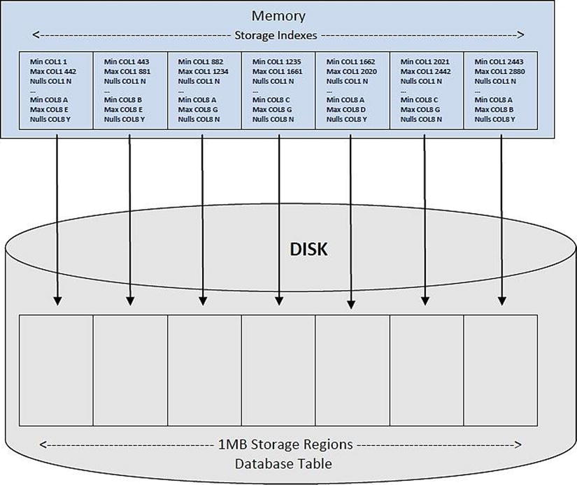
Figure 3-1. Storage index structure
Each storage segment for a table is associated with a memory region in each storage cell; each memory region contains the index data for the table storage segment it is mapped to. As Oracle processes a Smart Scan it also scans these index regions, looking for possible matches (segments that could contain the desired value or values) while skipping the segments it can ignore (those having no possibility of containing the desired value). It’s the ability to skip reading “unnecessary” data segments, segments where the desired data cannot be found, that gives storage indexes their power.
Given that glorious, although long, description, it isn’t difficult to understand why storage indexes can be confusing. But they don’t need to be.
Don’t Look Here
Unlike a B-tree index, designed and implemented to tell Oracle where data is , a storage index is designed to allow Oracle to skip, or bypass, storage segments, basically telling Oracle where data isn’t. To explain further, a B-tree index contains the exact value or values indexed, plus the rowid for each row in the table. The presence of the rowid pinpoints where the particular index key is found, allowing Oracle to zero in on the precise location for the desired key or keys. Thus, a B-tree index reports the exact location for each index key. Storage indexes have no exact locations stored.
For each offloaded query, a Smart Scan will use a storage index, provided one is available. Remember: These are dynamically created when predicates are offloaded to the storage cells, so some tables may not have a storage index created yet. When one exists, Oracle, through the storage cells, will scan a storage index and see if the column or columns of interest are present and whether the desired value falls within the minimum/maximum range recorded for the column or columns in a given segment. If the column is indexed and the desired value falls outside of the recorded range, that 1MB segment is skipped, creating instant I/O savings.
A storage index will also be used by IS NULL and IS NOT NULL predicates, because there is a bit set to indicate the presence of NULL values in an index segment. Depending on the data, a query either looking for or avoiding NULL values could bypass most of the table data, making the result set return much more quickly than on a conventionally configured system. A query must qualify for a Smart Scan before it will use a storage index; thus, it must meet all of the criteria for Smart Scan execution. Those conditions are listed in the previous chapter, so they won’t be repeated here.
An interesting aspect of a storage index is its effectiveness, which is based on the location of key data in the table. For a conventional B-tree index, this is called the Clustering Factor, a function of how far Oracle must “trave” in the table to arrive at the location of the next key in the index. As one would expect, a fairly low value for the Clustering Factor is a good thing; unfortunately, that can only be guaranteed if the table data is ordered by the index key. Ordering the data to improve the Clustering Factor for one index most often makes the Clustering Factors for any remaining indexes worse. Likewise, a storage index has a pseudo–“Clustering Factor” in that the location of indexed key values can affect how well a storage index is used and whether or not it provides real I/O savings. Unlike with a B-tree index, clustering the keys close to each other in the table enhances the performance, and since there is only one storage index per table, adverse effects are few. Of course, after the initial data loading of a heap table, there is no guarantee that the ordering will be preserved, as inserts and deletes can shift the data keys outside of the desired groupings. Still, it would take a tremendous volume of inserts and deletes to entirely undo the key clustering that was originally established.
Remember that cell maintenance will cause storage index segments to be lost, forcing storage index creation from offloaded predicates once the cell or cells are back online. If those predicates create storage index segments different from those that were lost, the originally established key clustering may no longer be beneficial. Situations wherein the search key is scattered across the entire table can result in a 0 byte savings for the query, as there may be no segment that does not contain the desired value within the specified range. Table data relatively clustered with respect to the search key provides varying degrees of I/O reduction, depending on how closely the search keys are grouped. Low cardinality columns, those containing values such as True, False, Yes, No, or limited-range numeric values fare better when clustered than columns having a wide range of values or columns enforcing Unique and Primary Key constraints. Examples in the next two sections use a low cardinality column (SUITABLE_FOR_FRYING) containing one of two values, “Yes” and “No,” to illustrate both conditions.
I Used It
To know if a storage index has provided any benefit to a query, a statistic, “cell physical IO bytes saved by storage index,” will record the bytes the storage index allowed Oracle to bypass. This is a cumulative metric, meaning that the prior value is incremented each time the storage index allowed Oracle to skip reading data segments in the currently connected session (as reported by V$MYSTAT) or for a given session (in GV$SESSTAT). (Creating a new session or reestablishing a connection [using “connect <user>/<pass>” at the SQL> prompt] will reset the session-level counter.)
To illustrate this, two queries will be executed, after some initial setup not shown in the examples, that illustrate that a storage index allowed Oracle to skip reading data and that the byte savings value reported by Oracle is, indeed, cumulative. The storage_index_ex.sql script was used to generate this output, and running this on your own system will display the setup as well as the output shown here, plus the parts that were edited owing to their size. The log file this script generates is extremely large; it does include both sets of examples, however, and requires only a single execution to provide the entire set of results. The second example, run immediately after the first and starting with reconnecting as the schema owner, executes the same two queries. The connections will be reestablished between the two statements, which will show the actual savings for each query.
Two tables are created and populated, then the queries are run; the following shows the results of that first run:
SQL> select /*+ parallel(4) */
  2  count(*)
  3  from chicken_hr_tab
  4  where suitable_for_frying = 'Yes';

  COUNT(*)
----------
   2621440

SQL> select *
  2  from v$mystat
  3  where statistic# = (select statistic# from v$statname where name = 'cell physical
      IO bytes saved by storage index'),

       SID STATISTIC#      VALUE
---------- ---------- ----------
      1107        247 1201201152

SQL> select /*+ parallel(4) */
  2  chicken_id, chicken_name, suitable_for_frying
  3  from chicken_hr_tab
  4  where suitable_for_frying = 'Yes';

CHICKEN_ID CHICKEN_NAME         SUI
---------- -------------------- ---
  38719703 Frieda               Yes
  38719704 Edie                 Yes
  38719705 Eunice               Yes
...
  37973451 Eunice               Yes
  37973452 Fran                 Yes

2621440 rows selected.

SQL> select *
  2  from v$mystat
  3  where statistic# = (select statistic# from v$statname where name = 'cell physical
      IO bytes saved by storage index'),

       SID STATISTIC#      VALUE
---------- ---------- ----------
      1107        247 2281971712

SQL>
For the first query, approximately 1GB of data was bypassed to provide the record count; the second query skipped an additional 1GB of table data. That isn’t obvious from the output shown, as the value displayed is, as noted before, the cumulative result. You may not need to know the bytes skipped by each query, so the cumulative count could be exactly what you want. The cumulative count, though, will also display unchanged for queries that do not execute a Smart Scan, so careful attention must be paid to the output of the V$MYSTAT query. If you do want individual savings figures, then you can produce those results as well; in this case, queries that do not meet Smart Scan criteria will return a 0 byte total. As noted previously, the script reconnects between queries; this produces results that better illustrate the I/O savings the storage index provides on a per-query basis:
SQL> connect bing/#######
Connected.
SQL> select /*+ parallel(4) */
  2  count(*)
  3  from chicken_hr_tab
  4  where suitable_for_frying = 'Yes';

  COUNT(*)
----------
   2621440

SQL> select *
  2  from v$mystat
  3  where statistic# = (select statistic# from v$statname where name = 'cell physical
      IO bytes saved by storage index'),

       SID STATISTIC#      VALUE
---------- ---------- ----------
      1233        247 1080770560

SQL> connect bing/#######
Connected.
SQL> select /*+ parallel(4) */
  2  chicken_id, chicken_name, suitable_for_frying
  3  from chicken_hr_tab
  4  where suitable_for_frying = 'Yes';

CHICKEN_ID CHICKEN_NAME         SUI
---------- -------------------- ---
  38719703 Frieda               Yes
  38719704 Edie                 Yes
...
  37973451 Eunice               Yes
  37973452 Fran                 Yes

2621440 rows selected.

SQL>
SQL> select *
  2  from v$mystat
  3  where statistic# = (select statistic# from v$statname where name = 'cell physical
      IO bytes saved by storage index'),

       SID STATISTIC#      VALUE
---------- ---------- ----------
      1233        247 1080770560

SQL>
Now it’s obvious how much data was skipped for each query. For the initial run, there were also 120,430,592 bytes skipped when loading the data. (After the initial insert statements were executed, a series of “insert into . . . select . . . from . . .” statements were used to further populate the table.) The second run shows the actual savings the storage index provided for each query.
Oracle can skip table segments based on information the storage index provides, but because the index data is very basic, some “false positives” can occur. Oracle may find that a given segment satisfies the search criteria, because the searched-for value falls between the minimum and maximum values recorded for that segment, but, in reality, the minimum and maximum values hide the fact that the actual desired value does not exist in that particular segment.
In such cases, Oracle reads through the segment and comes up empty-handed, as no rows meeting the exact query criteria were found, even though the storage index indicated otherwise. Depending on how well grouped the keys are in the table, more segments than one would expect could be read, segments that produce no results, because the indexed values “falsely” indicate that a row or rows may exist. In this next example, a count of records having a TALENT_CD of 4 is desired. The data is loaded so that TALENT_CD values 3 and 5 are placed in the same table segments, and the rest of the TALENT_CD values are loaded into the remaining segments. This will provide the conditions to create a “false positive” result from the storage index:
SQL> insert /*+ append */
  2  into chicken_hr_tab (chicken_name, talent_cd, retired, retire_dt, suitable_for_frying, fry_dt)
  3  select
  4  chicken_name, talent_cd, retired, retire_dt, suitable_for_frying, fry_dt from chicken_hr_tab2
  5  where talent_cd in (3,5);

1048576 rows created.

Elapsed: 00:01:05.10
SQL> commit;

Commit complete.

Elapsed: 00:00:00.01
SQL> insert /*+ append */
  2  into chicken_hr_tab (chicken_name, talent_cd, retired, retire_dt, suitable_for_frying, fry_dt)
  3  select
  4  chicken_name, talent_cd, retired, retire_dt, suitable_for_frying, fry_dt from chicken_hr_tab2
  5  where talent_cd not in (3,5);

37748736 rows created.

Elapsed: 00:38:09.12
SQL> commit;

Commit complete.

Elapsed: 00:00:00.00
SQL>
SQL> exec dbms_stats.gather_table_stats(user, 'CHICKEN_TALENT_TAB', cascade=>true, estimate_percent=>null);

PL/SQL procedure successfully completed.

Elapsed: 00:00:00.46
SQL> exec dbms_stats.gather_table_stats(user, 'CHICKEN_HR_TAB', cascade=>true, estimate_percent=>null);

PL/SQL procedure successfully completed.

Elapsed: 00:00:31.66
SQL>
SQL> set timing on
SQL>
SQL> connect bing/bong0$tar
Connected.
SQL> alter session set parallel_force_local=true;

Session altered.

Elapsed: 00:00:00.00
SQL> alter session set parallel_min_time_threshold=2;

Session altered.

Elapsed: 00:00:00.00
SQL> alter session set parallel_degree_policy=manual;

Session altered.

Elapsed: 00:00:00.00
SQL>
SQL>
SQL> set timing on
SQL>
SQL> select /*+ parallel(4) */
  2  chicken_id
  3  from chicken_hr_tab
  4  where talent_cd = 4;

     CHICKEN_ID
---------------
       60277401
       60277404
...
       72320593
       72320597
       72320606
       72320626

4718592 rows selected.

Elapsed: 00:03:17.92
SQL>
SQL> select *
  2  from v$mystat
  3  where statistic# = (select statistic# from v$statname where name = 'cell physical
      IO bytes saved by storage index'),

            SID      STATISTIC#           VALUE
--------------- --------------- ---------------
            915             247               0

Elapsed: 00:00:00.01
SQL>
![]() Note The manner in which the data was loaded set the minimum and maximum values for TALENT_CD such that the storage index could not ignore any of the blocks, even though there are segments that do not contain the desired value.
Note The manner in which the data was loaded set the minimum and maximum values for TALENT_CD such that the storage index could not ignore any of the blocks, even though there are segments that do not contain the desired value.
The minimum and maximum values stored for an indexed segment don’t guarantee that the desired value will be found, just that there is a high probability that the value exists in the associated table segment.
Even though this example was intentionally created to provide such a condition, it is also likely that this could occur in a production system, as normally occurring data changes (through inserts, updates, and deletes) could create this same sort of situation.
Or Maybe I Didn’t
Data clustering plays a big part in whether a storage index provides any benefit. In the preceding example, great care was taken to load the data in a manner that would make a storage index beneficial to the query. Values of interest (those in the WHERE clause) were loaded, so that one or more of the 1MB table segments storage indexes operate upon contained values that could be skipped. In the next example, data was loaded in a fairly fast and convenient manner; the initial table population resulted in rows containing the value of interest (SUITABLE_FOR_FRYING is 'Yes') being scattered across the table and thus being found in every 1MB storage index segment. Subsequent loading of the data, using a simple “insert into . . . select from . . .” syntax, preserved that scattering and rendered the storage index basically useless for the given query. (It is a common practice to consider that a storage index was “not used” when the “cell physical IO bytes saved by storage index” statistic is 0, which isn’t true. The storage index was used; there is no question about that, but it provided no benefit in the form of reduced I/O, as Oracle could not skip any of the 1MB data segments in its search for the desired rows.) Looking at the run where the storage index “key” data was scattered across the entire table, the following results were seen:
SQL> select /*+ parallel(4) */
  2  count(*)
  3  from chicken_hr_tab
  4  where suitable_for_frying = 'Yes';

  COUNT(*)
----------
   2621440

SQL>
SQL> select *
  2  from v$mystat
  3  where statistic# = (select statistic# from v$statname where name = 'cell physical
      IO bytes saved by storage index'),

       SID STATISTIC#      VALUE
---------- ---------- ----------
      1304        247          0

SQL> select /*+ parallel(4) */
  2  chicken_id, chicken_name, suitable_for_frying
  3  from chicken_hr_tab
  4  where suitable_for_frying = 'Yes';

CHICKEN_ID CHICKEN_NAME         SUI
---------- -------------------- ---
  38699068 Pickles              Yes
  38699070 Frieda               Yes
  ...
  10116134 Pickles              Yes
  10116136 Frieda               Yes

2621440 rows selected.

SQL>
SQL> select *
  2  from v$mystat
  3  where statistic# = (select statistic# from v$statname where name = 'cell physical
      IO bytes saved by storage index'),

       SID STATISTIC#      VALUE
---------- ---------- ----------
      1304        247          0

SQL> select /*+ parallel(4) */
  2  h.chicken_name, t.talent, h.suitable_for_frying
  3  from chicken_hr_tab h join chicken_talent_tab t on (t.talent_cd = h.talent_cd)
  4  where h.talent_cd = 5;

CHICKEN_NAME         TALENT                                   SUI
-------------------- ---------------------------------------- ---
Cat                  Accountant                               No
Cat                  Accountant                               No
Cat                  Accountant                               No
Cat                  Accountant                               No
...
Cat                  Accountant                               No
Cat                  Accountant                               No

524288 rows selected.

SQL>
SQL> select *
  2  from v$mystat
  3  where statistic# = (select statistic# from v$statname where name = 'cell physical
     IO bytes saved by storage index'),

       SID STATISTIC#      VALUE
---------- ---------- ----------
      1304        247          0

SQL>
Since there is no 1MB segment that does not contain the searched-for value, the storage index cannot tell Oracle to skip any of them, which is reflected in the VALUE column from V$MYSTAT for the “cell physical IO bytes saved by storage index” statistic. (In 11.2.0.3, the statistic number for this event is 247, but it’s best to actually query on the statistic name, as Oracle can, and has, reassigned statistic numbers for existing statistics, as new ones are added in newer versions.) Again, this does not mean that this storage index was not used; it does mean that no I/O savings were realized by using it.
Execution Plan Doesn’t Know
Execution plans won’t report storage index usage, because, frankly, the optimizer doesn’t know whether a Smart Scan will or will not be used for a given query. The only certain monitoring method, outside of enabling tracing at the CELLSRV level, is through the “cell physical IO bytes saved by storage index” statistic. Chapter 9 will cover how to enable CELLSRV tracing; starting CELLSRV tracing requires a restart of the cell, which causes the storage index segments to be dropped.
Looking at the previous queries, showing (and not showing) storage index savings adding the execution plans to the generated output verifies that the optimizer won’t report any information on the storage indexes in use:
SQL> set autotrace on
SQL>
SQL> select /*+ parallel(4) */
  2  h.chicken_name, t.talent, h.suitable_for_frying
  3  from chicken_hr_tab h join chicken_talent_tab t on (t.talent_cd = h.talent_cd)
  4  where h.talent_cd = 5;

CHICKEN_NAME         TALENT                                   SUI
-------------------- ---------------------------------------- ---
Cat                  Accountant                               No
Cat                  Accountant                               No
Cat                  Accountant                               No
Cat                  Accountant                               No
Cat                  Accountant                               No
...
Cat                  Accountant                               No
Cat                  Accountant                               No
Cat                  Accountant                               No
Cat                  Accountant                               No

524288 rows selected.

Execution Plan
----------------------------------------------------------
Plan hash value: 793882093


Predicate Information (identified by operation id):
---------------------------------------------------

   6 - storage("H"."TALENT_CD"=5)
       filter("H"."TALENT_CD"=5)
   7 - access("T"."TALENT_CD"="H"."TALENT_CD")
       filter("T"."TALENT_CD"="H"."TALENT_CD")
  11 - storage("T"."TALENT_CD"=5)
       filter("T"."TALENT_CD"=5)

Note
-----
   - Degree of Parallelism is 4 because of hint

Statistics
----------------------------------------------------------
         25  recursive calls
          0  db block gets
     152401  consistent gets
     151444  physical reads
          0  redo size
    9018409  bytes sent via SQL*Net to client
     384995  bytes received via SQL*Net from client
      34954  SQL*Net roundtrips to/from client
          8  sorts (memory)
          0  sorts (disk)
     524288  rows processed

SQL>
SQL> set autotrace off
SQL>
SQL> select *
  2  from v$mystat
  3  where statistic# = (select statistic# from v$statname where name = 'cell physical
      IO bytes saved by storage index'),

       SID STATISTIC#      VALUE
---------- ---------- ----------
         3        247   92028928

SQL>
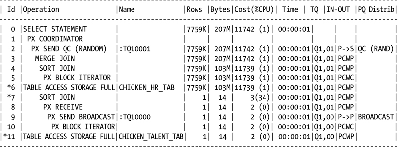
The only evidence of storage index usage is the output from the final query in this example. No mention of storage indexes appears in the execution plan output.
The More, the Merrier
Data distribution plays a large part in storage index performance, but that’s not the only data-related area that can impact Smart Scan execution and, as a result, storage index usage. Table size can also determine whether a storage index can be utilized. Serial direct path reads are generally utilized for large objects; small tables rarely trigger Smart Scans. How big does a table have to be to trigger a Smart Scan, and thus use a storage index? For the scripts shown here, the smallest table size that would guarantee a Smart Scan generated 40 extents, consuming 335,544,320 bytes. Smaller table sizes were tried, with no Smart Scans executed; however, with the loading method used, a smaller table size that would trigger a Smart Scan may not have been generated. Since exhaustive testing was not completed, there may be smaller tables that will trigger Smart Scan executions.
Size isn’t the only factor in whether a Smart Scan will be triggered. Partitioned tables can create an interesting situation where the overall table size is sufficient to trigger a Smart Scan, but the sizes of the individual partitions aren’t. Such a situation is created by the storage_index_part_ex.sql script. Again, the initial setup isn’t shown, in order to concentrate on the end results. There are five partitions created and populated for this version of the table, with a deliberate attempt to evenly spread the data across all of the partitions. The names and row counts for each partition are shown as follows:
SQL> select count(*) from chicken_hr_tab partition(chick1);
       COUNT(*)
---------------
        1966080

SQL> select count(*) from chicken_hr_tab partition(chick2);

       COUNT(*)
---------------
        1966080

SQL> select count(*) from chicken_hr_tab partition(chick3);

       COUNT(*)
---------------
        1966080

SQL> select count(*) from chicken_hr_tab partition(chick4);

       COUNT(*)
---------------
        1966080

SQL> select count(*) from chicken_hr_tab partition(chick5);

       COUNT(*)
---------------
        1835008

SQL>
Overall, the table is large enough to ensure that a Smart Scan will be executed, and if the query involves a large percentage of the table data, a Smart Scan will, indeed, be run. It’s the relatively small sizes of the individual partitions that can cause them to not qualify for a Smart Scan. Now that the stage is properly set, the same queries from the previous example are executed, and the Smart Scan results are reported. The changes between the examples are the partitioned table and the partition key distribution, which make a marked difference in Smart Scan execution and the benefit a storage index provides. The results, as Exadata reports them, are as follows:
SQL> select /*+ parallel(4) */
  2  count(*)
  3  from chicken_hr_tab
  4  where suitable_for_frying = 'Yes';

       COUNT(*)
---------------
         655360

SQL>
SQL> select *
  2  from v$mystat
  3  where statistic# = (select statistic# from v$statname where name = 'cell physical
      IO bytes saved by storage index'),

            SID      STATISTIC#           VALUE
--------------- --------------- ---------------
           1434             247       187088896

SQL>
SQL> select /*+ parallel(4) */
  2  chicken_id, chicken_name, suitable_for_frying
  3  from chicken_hr_tab
  4  where suitable_for_frying = 'Yes';

     CHICKEN_ID CHICKEN_NAME         SUI
--------------- -------------------- ---
        2411502 Frieda               Yes
...
        9507995 Fran                 Yes
        9507996 Eunice               Yes

655360 rows selected.

SQL>
SQL> select  sql_id,
  2  io_cell_offload_eligible_bytes qualifying,
  3  io_cell_offload_eligible_bytes - io_cell_offload_returned_bytes actual,
  4  round(((io_cell_offload_eligible_bytes - io_cell_offload_returned_bytes)/io_cell_offload_
     eligible_bytes)*100, 2) io_saved_pct,
  5  sql_text
  6  from v$sql
  7  where io_cell_offload_returned_bytes > 0
  8  and instr(sql_text, 'suitable_for_frying') > 0
  9  and parsing_schema_name = 'BING';

SQL_ID             QUALIFYING          ACTUAL    IO_SAVED_PCT
------------- --------------- --------------- ---------------
SQL_TEXT
---------------------------------------------------------------------------------------------------
8hgwndn3tj7xg       315211776       223167616            70.8
select /*+ parallel(4) */ chicken_id, chicken_name, suitable_for_frying from chicken_hr_tab where suitable_for_frying = 'Yes'

c1486fx9pv44n       315211776       230036536           72.98
select /*+ parallel(4) */ count(*) from chicken_hr_tab where suitable_for_frying = 'Yes'

9u65az96tvhj5        62111744        22646696           36.46
select /*+ parallel(4) */ h.chicken_name, t.talent, h.suitable_for_frying from chicken_hr_tab h join chicken_talent_tab t on (t.talent_cd = h.talent_cd) where h.talent_cd = 5

SQL>
SQL> select *
  2  from v$mystat
  3  where statistic# = (select statistic# from v$statname where name = 'cell physical
      IO bytes saved by storage index'),

            SID      STATISTIC#           VALUE
--------------- --------------- ---------------
           1434             247       282230784

SQL>

SQL> select /*+ parallel(4) */
  2  h.chicken_name, t.talent, h.suitable_for_frying
  3  from chicken_hr_tab h join chicken_talent_tab t on (t.talent_cd = h.talent_cd)
  4  where h.talent_cd = 5;

CHICKEN_NAME         TALENT                                   SUI
-------------------- ---------------------------------------- ---
Hazel                Accountant                               No
Red                  Accountant                               No
Amanda               Accountant                               No
Dolly                Accountant                               No
...
Terry                Accountant                               No
Beulah               Accountant                               No
Calcutta             Accountant                               No

1835008 rows selected.

SQL>
SQL> select  sql_id,
  2  io_cell_offload_eligible_bytes qualifying,
  3  io_cell_offload_eligible_bytes - io_cell_offload_returned_bytes actual,
  4  round(((io_cell_offload_eligible_bytes - io_cell_offload_returned_bytes)/io_cell_offload_     eligible_bytes)*100, 2) io_saved_pct,
  5  sql_text
  6  from v$sql
  7  where io_cell_offload_returned_bytes > 0
  8  and instr(sql_text, 'suitable_for_frying') > 0
  9  and parsing_schema_name = 'BING';

SQL_ID             QUALIFYING          ACTUAL    IO_SAVED_PCT
------------- --------------- --------------- ---------------
SQL_TEXT
---------------------------------------------------------------------------------------------------
8hgwndn3tj7xg       315211776       223167616            70.8
select /*+ parallel(4) */ chicken_id, chicken_name, suitable_for_frying from chicken_hr_tab where suitable_for_frying = 'Yes'

c1486fx9pv44n       315211776       230036536           72.98
select /*+ parallel(4) */ count(*) from chicken_hr_tab where suitable_for_frying = 'Yes'

9u65az96tvhj5        62242816        26925984           43.26
select /*+ parallel(4) */ h.chicken_name, t.talent, h.suitable_for_frying from chicken_hr_tab h join chicken_talent_tab t on (t.talent_cd = h.talent_cd) where h.talent_cd = 5

SQL>
So far, so good, as Smart Scans are being executed as expected. Reconnecting as the schema owner and adding another query, a different picture emerges. Between each query of the partitioned table, the session statistics are reset by again reconnecting as the schema owner, as follows:
SQL> connect bing/#########
Connected.
SQL>
SQL> select /*+ parallel(4) */
  2  count(*)
  3  from chicken_hr_tab
  4  where suitable_for_frying = 'Yes';

       COUNT(*)
---------------
         655360

SQL>
SQL> select  sql_id,
  2  io_cell_offload_eligible_bytes qualifying,
  3  io_cell_offload_eligible_bytes - io_cell_offload_returned_bytes actual,
  4  round(((io_cell_offload_eligible_bytes - io_cell_offload_returned_bytes)/io_cell_
     offload_eligible_bytes)*100, 2) io_saved_pct,
  5  sql_text
  6  from v$sql
  7  where io_cell_offload_returned_bytes > 0
  8  and instr(sql_text, 'suitable_for_frying') > 0
  9  and parsing_schema_name = 'BING';

SQL_ID             QUALIFYING          ACTUAL    IO_SAVED_PCT
------------- --------------- --------------- ---------------
SQL_TEXT
---------------------------------------------------------------------------------------------------
8hgwndn3tj7xg       315211776       223167616            70.8
select /*+ parallel(4) */ chicken_id, chicken_name, suitable_for_frying from chicken_hr_tab where suitable_for_frying = 'Yes'

c1486fx9pv44n       315211776       230036536           72.98
select /*+ parallel(4) */ count(*) from chicken_hr_tab where suitable_for_frying = 'Yes'

9u65az96tvhj5        62242816        26925984           43.26
select /*+ parallel(4) */ h.chicken_name, t.talent, h.suitable_for_frying from chicken_hr_tab h join chicken_talent_tab t on (t.talent_cd = h.talent_cd) where h.talent_cd = 5

SQL>

SQL> select *
  2  from v$mystat
  3  where statistic# = (select statistic# from v$statname where name = 'cell physical
      IO bytes saved by storage index'),

            SID      STATISTIC#           VALUE
--------------- --------------- ---------------
           1434             247        50757632

SQL>
SQL> connect bing/#########
Connected.
SQL>
SQL> select /*+ parallel(4) */
  2  sum(chicken_id)
  3  from chicken_hr_tab
  4  where suitable_for_frying = 'Yes';

SUM(CHICKEN_ID)
---------------
  4166118604642

SQL>
SQL> select  sql_id,
  2  io_cell_offload_eligible_bytes qualifying,
  3  io_cell_offload_eligible_bytes - io_cell_offload_returned_bytes actual,
  4  round(((io_cell_offload_eligible_bytes - io_cell_offload_returned_bytes)/io_cell_
     offload_eligible_bytes)*100, 2) io_saved_pct,
  5  sql_text
  6  from v$sql
  7  where io_cell_offload_returned_bytes > 0
  8  and instr(sql_text, 'suitable_for_frying') > 0
  9  and parsing_schema_name = 'BING';

SQL_ID             QUALIFYING          ACTUAL    IO_SAVED_PCT
------------- --------------- --------------- ---------------
SQL_TEXT
---------------------------------------------------------------------------------------------------
8hgwndn3tj7xg       315211776       223167616            70.8
select /*+ parallel(4) */ chicken_id, chicken_name, suitable_for_frying from chicken_hr_tab where suitable_for_frying = 'Yes'

c1486fx9pv44n       315211776       230036536           72.98
select /*+ parallel(4) */ count(*) from chicken_hr_tab where suitable_for_frying = 'Yes'

9u65az96tvhj5        62242816        26925984           43.26
select /*+ parallel(4) */ h.chicken_name, t.talent, h.suitable_for_frying from chicken_hr_tab h join chicken_talent_tab t on (t.talent_cd = h.talent_cd) where h.talent_cd = 5

SQL>
SQL> select *
  2  from v$mystat
  3  where statistic# = (select statistic# from v$statname where name = 'cell physical
      IO bytes saved by storage index'),

            SID      STATISTIC#           VALUE
--------------- --------------- ---------------
           1434             247               0

SQL>
SQL> connect bing/#########
Connected.
SQL>
SQL> select /*+ parallel(4) */
  2  chicken_id, chicken_name, suitable_for_frying
  3  from chicken_hr_tab
  4  where suitable_for_frying = 'Yes';

     CHICKEN_ID CHICKEN_NAME         SUI
--------------- -------------------- ---
        9539150 Frieda               Yes
        9539151 Frieda               Yes
...
        9489101 Eunice               Yes
        9489102 Eunice               Yes

655360 rows selected.

SQL>
SQL> select  sql_id,
  2  io_cell_offload_eligible_bytes qualifying,
  3  io_cell_offload_eligible_bytes - io_cell_offload_returned_bytes actual,
  4  round(((io_cell_offload_eligible_bytes - io_cell_offload_returned_bytes)/io_cell_
     offload_eligible_bytes)*100, 2) io_saved_pct,
  5  sql_text
  6  from v$sql
  7  where io_cell_offload_returned_bytes > 0
  8  and instr(sql_text, 'suitable_for_frying') > 0
  9  and parsing_schema_name = 'BING';

SQL_ID             QUALIFYING          ACTUAL    IO_SAVED_PCT
------------- --------------- --------------- ---------------
SQL_TEXT
---------------------------------------------------------------------------------------------------
8hgwndn3tj7xg       315211776       223167616            70.8
select /*+ parallel(4) */ chicken_id, chicken_name, suitable_for_frying from chicken_hr_tab where suitable_for_frying = 'Yes'

c1486fx9pv44n       315211776       230036536           72.98
select /*+ parallel(4) */ count(*) from chicken_hr_tab where suitable_for_frying = 'Yes'

9u65az96tvhj5        62242816        26925984           43.26
select /*+ parallel(4) */ h.chicken_name, t.talent, h.suitable_for_frying from chicken_hr_tab h join chicken_talent_tab t on (t.talent_cd = h.talent_cd) where h.talent_cd = 5

SQL>
SQL> select *
  2  from v$mystat
  3  where statistic# = (select statistic# from v$statname where name = 'cell physical
      IO bytes saved by storage index'),

            SID      STATISTIC#           VALUE
--------------- --------------- ---------------
           1434             247               0

SQL>
SQL> connect bing/#########
Connected.
SQL>
SQL> select /*+ parallel(4) */
  2  h.chicken_name, t.talent, h.suitable_for_frying
  3  from chicken_hr_tab h join chicken_talent_tab t on (t.talent_cd = h.talent_cd)
  4  where h.talent_cd = 5;

CHICKEN_NAME         TALENT                                   SUI
-------------------- ---------------------------------------- ---
Jennifer             Accountant                               No
Constance            Accountant                               No
Rachel               Accountant                               No
Katy                 Accountant                               No
...
Calcutta             Accountant                               No
Jennifer             Accountant                               No

1835008 rows selected.

SQL>
SQL> select  sql_id,
  2  io_cell_offload_eligible_bytes qualifying,
  3  io_cell_offload_eligible_bytes - io_cell_offload_returned_bytes actual,
  4  round(((io_cell_offload_eligible_bytes - io_cell_offload_returned_bytes)/io_cell_
     offload_eligible_bytes)*100, 2) io_saved_pct,
  5  sql_text
  6  from v$sql
  7  where io_cell_offload_returned_bytes > 0
  8  and instr(sql_text, 'suitable_for_frying') > 0
  9  and parsing_schema_name = 'BING';

SQL_ID             QUALIFYING          ACTUAL    IO_SAVED_PCT
------------- --------------- --------------- ---------------
SQL_TEXT
---------------------------------------------------------------------------------------------------
8hgwndn3tj7xg       315211776       223167616            70.8
select /*+ parallel(4) */ chicken_id, chicken_name, suitable_for_frying from chicken_hr_tab where suitable_for_frying = 'Yes'

c1486fx9pv44n       315211776       230036536           72.98
select /*+ parallel(4) */ count(*) from chicken_hr_tab where suitable_for_frying = 'Yes'

9u65az96tvhj5        62242816        26925984           43.26
select /*+ parallel(4) */ h.chicken_name, t.talent, h.suitable_for_frying from chicken_hr_tab h join chicken_talent_tab t on (t.talent_cd = h.talent_cd) where h.talent_cd = 5

SQL> select *
  2  from v$mystat
  3  where statistic# = (select statistic# from v$statname where name = 'cell physical
      IO bytes saved by storage index'),

            SID      STATISTIC#           VALUE
--------------- --------------- ---------------
           1434             247               0

SQL>
No benefit was realized from a storage index for the last query, because it didn’t execute a Smart Scan; the partitions are too small, individually, to trigger Smart Scan execution. Also, the first query computing the sum was not offloaded. This is proven by the fact that the query text is not listed among the SQL statements that were offloaded at one time or another, using another incarnation of the table and data.
NULLs
NULL searches are treated in a slightly different yet more efficient manner in Exadata. Unlike non-NULL table data, which is indexed by the minimum and maximum values for the listed column, the presence of NULLs is flagged by a bit for each column present in the storage index. Storage regions containing NULLs for the indexed columns have this bit set, which makes searching for NULLs a very fast operation, as Oracle only need search for segments where this NULL indicator bit shows that NULLs are present. Avoiding NULLs is also just as efficient, as Oracle only needs to read table segments where the NULL indicator bit is not set.
Proving this is another example, utilizing the previous data-loading strategy, clustering the desired values together to get the most “bang for the buck” out of the storage index. NULL values were added to the mix, so that three values now exist for the SUITABLE_FOR_FRYING column. Timing has been enabled to show the elapsed time for each query execution, so the total time for each query can be noted, and the session-level statistics were reset by reconnecting between queries, so it’s easier to see how many bytes the storage index skipped for each search condition:
SQL>
SQL> connect bing/#########
Connected.
SQL>
SQL> set timing on
SQL>
SQL> select /*+ parallel(4) */
  2  count(*)
  3  from chicken_hr_tab
  4  where suitable_for_frying = 'Yes';

       COUNT(*)
---------------
        1572864

Elapsed: 00:00:00.80
SQL>
SQL> select *
  2  from v$mystat
  3  where statistic# = (select statistic# from v$statname where name = 'cell physical
      IO bytes saved by storage index'),

            SID      STATISTIC#           VALUE
--------------- --------------- ---------------
           1111             247       566501376

Elapsed: 00:00:00.00
SQL>
SQL> connect bing/#########
Connected.
SQL>
SQL> set timing on
SQL>
SQL> select /*+ parallel(4) */
  2  count(*)
  3  from chicken_hr_tab
  4  where suitable_for_frying is null;

       COUNT(*)
---------------
        1048576

Elapsed: 00:00:00.23
SQL>
SQL> select *
  2  from v$mystat
  3  where statistic# = (select statistic# from v$statname where name = 'cell physical
      IO bytes saved by storage index'),

            SID      STATISTIC#           VALUE
--------------- --------------- ---------------
           1111             247      1141440512

Elapsed: 00:00:00.00
SQL>
The IS NULL query executed in less than one-third of the time required for the query searching for “employees” ready to be sent to the fryer and skipped almost twice the number of bytes, because very few of the table segments contain NULL values. Again, this speed is partly due to not having to check minimum and maximum values for the specified column. Using this strategy, “false positives” won’t occur, as Oracle doesn’t flag segments that may have NULLs, only those segments where NULLs are actually present.
Storage indexes are memory-resident structures. As long as there is power to the storage cells, those indexes remain valid. Of course, using memory instead of more permanent physical media makes these indexes transient and subject to maintenance windows, power outages, and memory-card failures. There is no method to back up a storage index, and there really is no need to do so, given that storage indexes take very little time to build. The build process is not, as mentioned previously, the resource-intensive operation that building a “permanent” index would be. Using the term rebuild to replace dropped storage indexes is, to our minds, a misnomer, as there is no script to build them, and it’s just as likely that the storage indexes built after a restart of the storage cells will not match the storage indexes in place prior to the outage.
Because storage indexes are built on data stored in 1MB segments, it doesn’t take long to scan that segment of the table to find the minimum and maximum values an indexed column contains and note whether NULL values can or do exist. Building storage indexes after an outage is not the same resource-intensive operation that creating more permanent indexes can be. Building or rebuilding a B-tree index, for example, can take hours and can noticeably consume CPU and disk resources, whereas building a storage index is hardly noticeable during the course of day-to-day operations, doesn’t hamper other sessions while it is being built, and completes in a mere fraction of the time. True, the information in a storage index is nothing like that of a B-tree index, but it doesn’t need to be to serve its intended purpose.
Each storage server, or cell, has its own storage indexes, so losing one cell won’t drop the indexes in the remaining cells, which means that only the storage indexes found in the problem cell will have to be created again. One of the good aspects of a storage index is that the index for each 1MB segment does not need to match the indexes representing the other table segments. Because tables are striped across the disks in a disk group, the table data is spread across all of the storage cells and, as a result, each table will have storage index segments in each of the storage cells. Issues with one cell won’t create a situation where no storage indexes exist, so queries can still benefit from the index segments in the unaffected cells. In addition, the redundancy in ASM places the redundant data on a different storage cell from the primary source. This allows Exadata to lose a storage cell or apply patches in a rolling manner and not lose access to data.
Patching and software upgrades are probably the most likely reasons for storage indexes to be built, as CELLSRV needs to be stopped before some patching operations or software upgrades can begin. The size and scope of patching or upgrades will determine the fate of the storage indexes: database server patching/upgrades won’t touch the storage cells, so storage indexes will remain intact, and patching/upgrades involving the storage tier or the entire Exadata machine will drop storage indexes. Firmware issues affecting physical disks will also cause storage index “rebuilds” as the storage cells themselves, including the operating system, will have to be restarted. True, storage firmware issues and Exadata upgrades are not common occurrences, but they can happen, so it’s good to remember that storage indexes will have to be built once the storage firmware has been patched or the storage servers have been upgraded, either as storage maintenance or as part of an entire Exadata patch/upgrade, and the storage cells have been rebooted.
Another reason for storage indexes to be re-created involves maintenance on the flash cache hardware, the Sun flash PCIe cards. Four of these cards are installed into each storage server, providing 384GB of flash storage. Occasionally, these units need maintenance or replacement, which results in the affected storage cell being powered down. Although not directly related to the storage, they are part of the storage-cell architecture, and it should be noted that flash cache problems can require downtime to correct.
Remember that a Smart Scan can occur without a storage index being present. Losing storage indexes to maintenance windows or power outages isn’t going to appreciably affect performance while they are being created. The time that they are missing will also be brief, as the first offloadable query after the storage cells are again up and running will start the build process all over again, and each subsequent offloaded query will contribute to those indexes until they are complete. It may not even be noticeable to the end users running queries, as time differences will likely be small in comparison to the previous runtimes when the storage indexes were available.
Things to Know
Storage indexes are memory-resident structures, not permanent database objects. They are built or modified dynamically when predicates are offloaded to the storage cells. Each index segment can index up to eight columns, plus the presence of NULLs, and index data segments that are 1MB in size. The index segments are built on a first-come, first-served basis; offloaded predicates are added to the index until the eight-column limit per segment is attained. More than one query can add columns to a storage index for a table. The index segments contain the column name, the minimum value for that segment, the maximum value for that segment, and whether or not that segment contains NULL values for the included column, indicated by a bit in the segment structure. When storage indexes exist, they are always used by Smart Scans; not every query can benefit from a storage index, though, as values may be scattered across the table segments, causing Oracle to read each segment. A storage index is like a probability matrix, indicating only the possibility that a value exists in the indexed table segment and, as such, “false positives” can occur. Such “false positives,” created when the minimum and maximum values for a column in an index segment bracket the desired value but the desired value is not actually present in that segment, can also cause Oracle to read every table segment and provide no byte savings.
A storage index isn’t like a conventional B-tree index: it isn’t used to find where data is; it’s used to know where data isn't. Scanning the minimum and maximum values for a column in a given storage segment can allow Oracle to eliminate locations to search. Since each storage index segment indexes a 1MB storage “chunk” of a table, creating a storage index is a fairly fast operation, done “on the fly” during query processing. Also, eliminating 1MB pieces of a table can quickly provide speed to a query: the less data Oracle needs to sift through, the faster the result set will be returned. In some ways, a storage index is really an anti-index, since it’s used to eliminate locations to search, rather than pinpoint exactly where the desired data resides.
NULL values are treated differently, and more efficiently, than non-NULL search criteria, as Oracle only needs to read the NULL bit in the index. This can speed up queries by eliminating storage segments much faster than assessing minimum and maximum value pairs. Queries using the IS NULL and IS NOT NULL comparison operators can often return in a fraction of the time of queries where actual data values are used.
How data is loaded into a table also affects how efficient and fast a storage index can be. Tables where like values are clustered together can eliminate more storage segments than if the data values of interest are scattered across the entire table. The fewer storage segments that contain the value or values of interest allow Oracle to eliminate more storage segments from being read, returning the results much faster than would be possible with random data loading. Of course it’s not possible to optimize storage indexes for every column they may contain, just as it isn’t possible to generate the optimal Clustering Factor for every B-tree index created against a table.
Size can play a big part in the creation of storage indexes, and partitioned tables, in particular, can suffer from realizing no benefit from a storage index, if the partition or partitions being queried are small with respect to the overall table size. Querying the entire table without using partition pruning would realize savings from the use of the storage index.
Monitoring storage index benefits from the database server is an easy task. A single statistic named “cell physical IO bytes saved by storage index” in the V$SESSTAT and V$MYSTAT views records the bytes saved in a cumulative fashion, for each session in V$SESSTAT and for the current session in V$MYSTAT. Logging out and logging in again, or using connect to establish a new session, will reset this statistic to 0. This can be a useful technique to report exactly how many bytes were saved for a particular query by executing a single query after each connect is made. It’s also useful to determine if any benefit was realized by using the storage index. Some queries won’t benefit, because they aren’t offloadable or the data was spread across every storage segment for the table or tables of interest.
Replacing storage indexes can be necessary for several reasons. Patching, software and/or hardware maintenance, and power outages are the major causes for this to occur. A less common cause for this is PCIe flash storage card maintenance or replacement, as that maintenance requires that the affected storage cell be powered down. Because they are basic indexes, containing a bare minimum of information, they are easy and fast to create and place very little load on the system. Only the affected storage cells will lose storage indexes, so if only one cell goes down, only those indexes will have to be built again.