
![]()
Final Thoughts
You’re here, at the final chapter of the book, and you’ve read and learned much by now. A lot of material has been covered, and you have a better idea of what Exadata is and what it can do. You also have a good working knowledge of the system and how to manage it. It was probably a daunting task at first, but, through reading this book and running the examples, you’ve gained an understanding of Exadata that will serve you well as you continue your career as an Exadata DBA or DMA.
You’ve Come Far, Pilgrim
When you started reading, you had probably just been told that Exadata was on its way and that you would be working with it. It’s also likely that you had no real idea of how Exadata is configured or how it provided the exceptional performance everyone was talking about. Storage indexes and Smart Scans were foreign concepts, and the architecture of the system was like nothing you had seen before. You have come a long way since then.
Let us take a walk through the areas we have covered and highlight some of the material we have presented.
![]() Note This will not be a comprehensive list of all of the topics and material we have presented in previous chapters. Information on some areas may be more detailed than others, but know this chapter is not a comprehensive summary of the text.
Note This will not be a comprehensive list of all of the topics and material we have presented in previous chapters. Information on some areas may be more detailed than others, but know this chapter is not a comprehensive summary of the text.
We started, appropriately enough, at the beginning, and discussed the various configurations of an Exadata system. We did this to get you introduced to the hardware available on each of the currently available systems and to familiarize you with the resources available on each configuration. We also presented a short history of Exadata and how it has evolved to address different types of workloads, including OLTP.
The next stop on this journey took you to Smart Scans and offloading, two very important aspects of Exadata.
It has been said that Smart Scans are the lifeblood of Exadata, and we would agree. Smart Scans, as you learned, provide a “divide and conquer” approach to query and statement processing, by allowing the storage cells to perform tasks that, in conventional hardware configurations, the database server would have to perform. You also learned that offloading provides even more powerful tools to make data processing more efficient. Column Projection and Predicate Filtering allow the storage cells to return only the data requested by the query, by moving the data block processing to the storage layer. Column Projection, as you recall, allows Exadata to return only the columns requested in the select list and any columns specified in join conditions. This reduces the workload considerably, by eliminating the need for the database servers to perform conventional data block processing and filtering. This also reduces the volume of data transferred to the database servers, which is one way Exadata is more efficient than conventionally configured systems.
Predicate Filtering improves this performance even further, by returning data from only the rows of interest, based on the predicates provided. Other conditions necessary for Smart Scan execution were covered, including direct-path reads and full-table or index scans. Execution plans were explained, so that you would know what information to look for to indicate that Smart Scans were, indeed, being used, and other metrics were provided to further prove Smart Scan use. These additional metrics include the storage keyword in the Predicate information and two columns from the V$SQL/GV$SQL pair of views, io_cell_offload_eligible_bytes and io_cell_offload_returned_bytes. The following example, first offered in Chapter 2, shows how these column values provide Smart Scan execution information.
SQL>select  sql_id,
  2         io_cell_offload_eligible_bytes qualifying,
  3         io_cell_offload_eligible_bytes - io_cell_offload_returned_bytes actual,
  4         round(((io_cell_offload_eligible_bytes -
io_cell_offload_returned_bytes)/io_cell_offload_eligible_bytes)*100, 2) io_saved_pct,
  5         sql_text
  6  from v$sql
  7  where io_cell_offload_returned_bytes> 0
  8  and instr(sql_text, 'emp') > 0
  9  and parsing_schema_name = 'BING';

SQL_ID        QUALIFYING     ACTUAL IO_SAVED_PCT SQL_TEXT
------------- ---------- ---------- ------------ -------------------------------------
gfjb8dpxvpuv6  185081856   42510928        22.97 select * from emp where empid = 7934

SQL>
We also covered Bloom filters and how Exadata uses them to improve join processing. Bloom filters are part of the offloading process for qualifying joins, and their use makes joins more efficient. You can see that Bloom filters are in use through the execution plan for a qualifying query, as the following example, again first provided in Chapter 2, illustrates.
Execution Plan
----------------------------------------------------------
Plan hash value: 2313925751


Predicate Information (identified by operation id):
---------------------------------------------------

   7 - access("ED"."EMPID"="E"."EMPID")
  15 - access("D"."DEPTNUM"=20)
  17 - storage("ED"."EMPDEPT"=20)
       filter("ED"."EMPDEPT"=20)
  19 - storage(SYS_OP_BLOOM_FILTER(:BF0000,"E"."EMPID"))
       filter(SYS_OP_BLOOM_FILTER(:BF0000,"E"."EMPID"))

Note
-----
   - dynamic sampling used for this statement (level=2)


Statistics
----------------------------------------------------------
     60  recursive calls
    174  db block gets
  40753  consistent gets
  17710  physical reads
   2128  redo size
9437983  bytes sent via SQL*Net to client
 183850  bytes received via SQL*Net from client
  16668  SQL*Net roundtrips to/from client
      6  sorts (memory)
      0  sorts (disk)
 250000  rows processed

SQL>
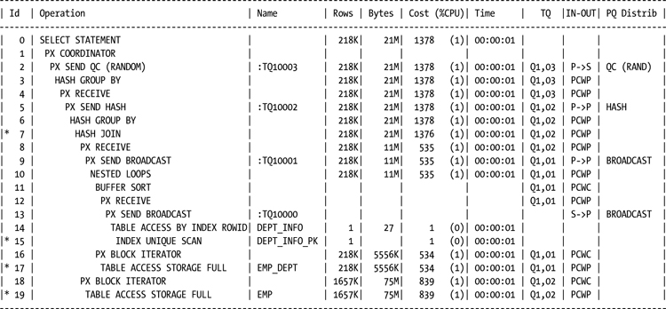
The presence of the SYS_OP_BLOOM_FILTER function in the plan output indicates the join was offloaded.
Functions can also be offloaded if they are found in the V$SQLFN_METADATA view; functions not found in this list will disqualify a query or statement from Smart Scan execution. Virtual columns can also be offloaded, which qualifies tables defined with virtual columns for Smart Scan execution.
Storage indexes were discussed in Chapter 3, and they are probably the most confusing aspect of Exadata, because this type of index is used to tell Oracle where not to look for data. Designed to assist in offload processing, storage indexes can significantly reduce the volume of data Oracle reads, by eliminating 1MB sections of table data. You learned that a storage index contains the barest minimum of data. You also learned that even though a storage index is small, it is undeniably mighty. Used to skip over 1MB sections where the desired data is not found, the resulting savings can be great. Of course, the good also comes with the bad, as a storage index can provide false positives, so that Oracle reads 1MB sections it doesn’t need to, because the desired value falls within the minimum/maximum range recorded in the storage index, even though the actual value doesn’t exist in that 1MB section of the table. To refresh your memory, the following example illustrates this.
SQL> insert /*+ append */
  2  into chicken_hr_tab (chicken_name, talent_cd, retired, retire_dt, suitable_for_frying, fry_dt)
  3  select
  4  chicken_name, talent_cd, retired, retire_dt, suitable_for_frying, fry_dt from chicken_hr_tab2
  5  where talent_cd in (3,5);

1048576 rows created.

Elapsed: 00:01:05.10
SQL> commit;

Commit complete.

Elapsed: 00:00:00.01
SQL> insert /*+ append */
  2  into chicken_hr_tab (chicken_name, talent_cd, retired, retire_dt, suitable_for_frying, fry_dt)
  3  select
  4  chicken_name, talent_cd, retired, retire_dt, suitable_for_frying, fry_dt from chicken_hr_tab2
  5  where talent_cd not in (3,5);

37748736 rows created.

Elapsed: 00:38:09.12
SQL> commit;

Commit complete.

Elapsed: 00:00:00.00
SQL>
SQL> exec dbms_stats.gather_table_stats(user, 'CHICKEN_TALENT_TAB', cascade=>true, estimate_percent=>null);

PL/SQL procedure successfully completed.

Elapsed: 00:00:00.46
SQL> exec dbms_stats.gather_table_stats(user, 'CHICKEN_HR_TAB', cascade=>true, estimate_percent=>null);

PL/SQL procedure successfully completed.

Elapsed: 00:00:31.66
SQL>
SQL> set timing on
SQL>
SQL> connect bing/#########
Connected.
SQL> alter session set parallel_force_local=true;

Session altered.

Elapsed: 00:00:00.00
SQL> alter session set parallel_min_time_threshold=2;

Session altered.

Elapsed: 00:00:00.00
SQL> alter session set parallel_degree_policy=manual;

Session altered.

Elapsed: 00:00:00.00
SQL>
SQL>
SQL> set timing on
SQL>
SQL> select /*+ parallel(4) */
  2  chicken_id
  3  from chicken_hr_tab
  4  where talent_cd = 4;

     CHICKEN_ID
---------------
       60277401
       60277404
...
       72320593
       72320597
       72320606
       72320626

4718592 rows selected.

Elapsed: 00:03:17.92
SQL>
SQL> select *
  2  from v$mystat
  3  where statistic# = (select statistic# from v$statname where name = 'cell physical IO bytes saved by storage index'),

            SID      STATISTIC#           VALUE
--------------- --------------- ---------------
            915             247               0

Elapsed: 00:00:00.01
SQL>
We feel this is a small price to pay for such efficiency.
Chapter 4 brought us to the Smart Flash Cache, a very versatile feature of Exadata, as it can be used as a read-through cache, a write-back cache, and even configured as flash disk usable by ASM. In addition to this functionality range, the Smart Flash Cache also has a portion configured as Smart Flash Log to make redo log processing more efficient. Log writes are processed both to disk, via the log groups, and to the Smart Flash Log, and the writes that finish first signal to Oracle that log processing has successfully completed. This allows Oracle to continue transaction processing at a potentially faster rate than using redo logs alone.
Chapter 5 brought us to parallel processing, an area that in conventionally configured systems can be both a help and a hindrance. Oracle 11.2.0.x provides improvements in the implementation and execution of parallel statements, which are available on any Exadata or non-Exadata configuration running this release of Oracle. It is the fact that Exadata was originally designed for data warehouse workloads, workloads that rely on parallel processing to speed the workflow, that makes it the ideal choice for parallel processing.
Certain configuration settings are necessary to enable the automatic parallel processing functionality, and a very important task, I/O calibration, is necessary for Exadata to actually act on these configuration settings. I/O calibration is a resource-intensive process and should not be run on systems during periods of heavy workloads. A packaged procedure, dbms_resource_manager.calibrate_io is provided to perform this task. Once the I/O calibration is complete, you will have to verify the parameters and settings found in Table 5-1 and Table 5-2.
Once you have everything set, you let Oracle take the reins; the users then reap the benefits of this improved parallel processing functionality. One of those benefits is parallel statement queuing, where Oracle will defer execution of a parallelized statement until sufficient resources are available. Querying the V$SQL_MONITOR view (or GV$SQL_MONITOR, to examine statements from all nodes in the cluster), where the status is QUEUED, will provide a list of statements waiting for sufficient resources to be released by parallel statements that finish execution. Provided you have set the resource limits correctly, this prevents the system from being overloaded, a vast improvement over the earlier parallel adaptive multiuser mechanism.
Another benefit is that Oracle will dynamically set the degree of parallelism (DOP) based on the available resources. One important item to note is that once the DOP is set by Oracle, it cannot be changed during execution, even if additional resources become available. The DOP is computed based on the estimated serial execution time for the given statement. A parameter, parallel_min_time_threshold, sets the threshold for serial execution time that will be the deciding factor for parallel execution. Remember that you can control whether queuing is enabled by setting the hidden parameter _parallel_statement_queuing to FALSE.
Another aspect of parallel execution is in-memory parallel execution. On the one hand, this can be desirable behavior, as disk I/O and traffic between the database servers and storage cells is eliminated, and the latency of memory is far lower than that for disk access. On the other hand, when this is active, Smart Scan optimizations are no longer available, because disk I/O is eliminated. Because the Smart Scan optimizations are eliminated, the database servers must perform all of the read processing that the storage cells would do, which increases the CPU usage. We also noted that we have not experienced in-memory parallel execution on any Exadata systems we’ve managed.
On to compression in Chapter 6. Exadata offers compression options not available on any non-Exadata platform, notably the Hybrid Columnar Compression (HCC) options. Those options are QUERY HIGH, QUERY LOW, ARCHIVE HIGH, and ARCHIVE LOW. These can significantly reduce the size of the selected tables; however, the compressed tables should be either inactive or subject to batch processing, including recompression, outside of the normal work hours. If HCC is used on actively updated tables, the compression level is silently changed to OLTP, and the original space savings are lost. Another aspect of using HCC is with respect to disaster recovery. If the recovery method is to simply restore the last good backup to a non-Exadata server or a server not using Exadata storage, the database could be unusable after the restore completes, because HCC isn’t supported on non-Exadata storage. This is a situation correctable by uncompressing the tables, but by correcting it, you may run into space issues, if the destination server tablespaces were created based on the compressed size of the Exadata database.
Table 6-3 and Table 6-4 in Chapter 6 list the estimated and actual compression ratios for the various compression methods, including OLTP. Those tables will not be reproduced here, but it is a good idea to look at them again, if you are contemplating using a compression method to save space.
Wait events specific to Exadata were covered in Chapter 7. These wait events report on cell-related wait information. Seven of these wait events collect wait data under the I/O wait category, and the cell statistics gather event seems to be incorrectly included in this category. The cell single block physical read and cell multiblock physical read events essentially replace the older db file sequential read and db file scattered read events, respectively.
RMAN has Exadata-specific waits as well: cell smart incremental backup and cell smart restore from backup. The first wait collects time against incremental Level 1 backups and the second accrues wait time experienced by an RMAN restore. Because a Level 0 incremental is, essentially, a full backup, wait times experienced for those backups is not recorded.
Performance counters and metrics specific to Exadata were covered in Chapter 8. The intent of that chapter was to provide an overview of what metrics and counters are available, what they mean, and when you should consider using them.
The cell metrics provide insight into statement performance and how Exadata executes statements. Dynamic counters such as cell blocks processed by data layer and cell blocks processed by index layer show how efficient the storage cells are in their processing. These counters are incremented every time a storage cell can complete data-layer and index-layer processing without passing data back to the database layer. Two reasons for the cells to pass data back to the database servers are consistent-read processing requiring undo blocks (regular block I/O) and chained-row processing where the chained pieces span storage cells. While the first condition can’t be controlled entirely (transactions can be so large as to exceed the automatic block-cleaning threshold), the second, chained rows, can be addressed and possibly corrected.
The cell num fast response sessions and cell num fast response sessions continuing to smart scan counters reveal the number of times Oracle chose to defer a Smart Scan in favor of regular block I/O, as an attempt to return the requested data with a minimum of work (the first listed counter), and how many times Oracle actually started a Smart Scan after the fast response session failed to return the requested data. These can give you insight into the nature of the statements submitted to your Exadata databases, by showing how often Smart Scans were averted because a small regular block I/O operation returned the requested data.
V$SQL also provides data that can be used to determine statement efficiency in the IO_CELL_OPFLOAD_ELIGIBLE_BYTES and IO_CELL_OFFLOAD_RETURNED_BYTES columns. These two columns can be used to calculate a percentage savings effected by a Smart Scan for a given query.
Chapter 9 went into storage cell monitoring, a very important aspect of Exadata, because some of the metrics are not passed back to the database servers. There are two accounts available outside of “root,” and those are cellmonitor and celladmin. Which one you use really depends on what tasks have to be accomplished.
The cellmonitor account has access to the cell metrics and counters and can generate monitoring reports. It has limited access at the O/S level and cannot execute any of the administrative commands or functions from cellcli, the cell command-line interface. Basically speaking, the LIST commands are available to cellmonitor, and those are sufficient for monitoring the cells and verifying that they are functioning properly.
The celladmin account, as you would expect, has more power. In addition to generating reports like cellmonitor, it has the ability to execute the series of ALTER, ASSIGN, DROP, EXPORT, and IMPORT commands.
Besides cellcli, the storage cells can be monitored with cellsrvstat and, from any node in the cluster, dcli. The cellcli utility can also be run directly from the command line, by passing to it the command you wish to execute, as the following example illustrates.
[celladmin@myexa1cel03 ∼]$ cellcli -e "list flashcache detail"
         name:                   myexa1cel03_FLASHCACHE
         cellDisk:               FD_00_myexa1cel03,FD_11_myexa1cel03,FD_02_myexa1cel03,FD_09_
myexa1cel03,FD_06_myexa1cel03,FD_14_myexa1cel03,FD_15_myexa1cel03,FD_03_myexa1cel03,FD_05_
myexa1cel03,FD_10_myexa1cel03,FD_07_myexa1cel03,FD_01_myexa1cel03,FD_13_myexa1cel03,FD_04_
myexa1cel03,FD_08_myexa1cel03,FD_12_myexa1cel03
         creationTime:           2012-08-28T14:15:50-05:00
         degradedCelldisks:
         effectiveCacheSize:     364.75G
         id:                     95f4e303-516f-441c-8d12-1795f5024c70
         size:                   364.75G
         status:                 normal
[celladmin@myexa1cel03 ∼]$
Using dcli from any of the database nodes, you can query all of the storage cells or a subset of them. Two options control how may cells will be polled: the -g option, where you pass a group file to dcli that contains all of the storage cell names, and the -c option, where you can specify, on the command line, a list of storage cells you want information from. When Exadata is configured, a group file named cell_group, among others, is created and can be used to poll all available storage cells, as follows:
[oracle@myexa1db01] $ dcli -g cell_group cellcli -e "list flashcache detail"
myexa1cel01: name:                       myexa1cel01_FLASHCACHE
myexa1cel01: cellDisk:                   FD_07_myexa1cel01,FD_12_myexa1cel01,FD_15_
myexa1cel01,FD_13_myexa1cel01,FD_04_myexa1cel01,FD_14_myexa1cel01,FD_00_myexa1cel01,FD_10_
myexa1cel01,FD_03_myexa1cel01,FD_09_myexa1cel01,FD_02_myexa1cel01,FD_08_myexa1cel01,FD_01_
myexa1cel01,FD_05_myexa1cel01,FD_11_myexa1cel01,FD_06_myexa1cel01
myexa1cel01: creationTime:               2013-03-16T12:16:39-05:00
myexa1cel01: degradedCelldisks:
myexa1cel01: effectiveCacheSize:         364.75G
myexa1cel01: id:                         3dfc24a5-2591-43d3-aa34-72379abdf3b3
myexa1cel01: size:                       364.75G
myexa1cel01: status:                     normal
myexa1cel02: name:                       myexa1cel02_FLASHCACHE
myexa1cel02: cellDisk:                   FD_04_myexa1cel02,FD_15_myexa1cel02,FD_02_
myexa1cel02,FD_11_myexa1cel02,FD_05_myexa1cel02,FD_01_myexa1cel02,FD_08_myexa1cel02,FD_14_
myexa1cel02,FD_13_myexa1cel02,FD_07_myexa1cel02,FD_03_myexa1cel02,FD_09_myexa1cel02,FD_12_
myexa1cel02,FD_00_myexa1cel02,FD_06_myexa1cel02,FD_10_myexa1cel02
myexa1cel02: creationTime:               2013-03-16T12:49:04-05:00
myexa1cel02: degradedCelldisks:
myexa1cel02: effectiveCacheSize:         364.75G
myexa1cel02: id:                         a450958c-5f6d-4b27-a70c-a3877430b82c
myexa1cel02: size:                       364.75G
myexa1cel02: status:                     normal
myexa1cel03: name:                       myexa1cel03_FLASHCACHE
myexa1cel03: cellDisk:                   FD_00_myexa1cel03,FD_11_myexa1cel03,FD_02_
myexa1cel03,FD_09_myexa1cel03,FD_06_myexa1cel03,FD_14_myexa1cel03,FD_15_myexa1cel03,FD_03_
myexa1cel03,FD_05_myexa1cel03,FD_10_myexa1cel03,FD_07_myexa1cel03,FD_01_myexa1cel03,FD_13_
myexa1cel03,FD_04_myexa1cel03,FD_08_myexa1cel03,FD_12_myexa1cel03
myexa1cel03: creationTime:               2012-08-28T14:15:50-05:00
myexa1cel03: degradedCelldisks:
myexa1cel03: effectiveCacheSize:         364.75G
myexa1cel03: id:                         95f4e303-516f-441c-8d12-1795f5024c70
myexa1cel03: size:                       364.75G
myexa1cel03: status:                     normal
myexa1cel04: name:                       myexa1cel04_FLASHCACHE
myexa1cel04: cellDisk:                   FD_08_myexa1cel04,FD_10_myexa1cel04,FD_00_
myexa1cel04,FD_12_myexa1cel04,FD_03_myexa1cel04,FD_02_myexa1cel04,FD_05_myexa1cel04,FD_01_
myexa1cel04,FD_13_myexa1cel04,FD_04_myexa1cel04,FD_11_myexa1cel04,FD_15_myexa1cel04,FD_07_
myexa1cel04,FD_14_myexa1cel04,FD_09_myexa1cel04,FD_06_myexa1cel04
myexa1cel04: creationTime:               2013-07-09T17:33:53-05:00
myexa1cel04: degradedCelldisks:
myexa1cel04: effectiveCacheSize:         1488.75G
myexa1cel04: id:                         7af2354f-1e3b-4932-b2be-4c57a1c03f33
myexa1cel04: size:                       1488.75G
myexa1cel04: status:                     normal
myexa1cel05: name:                       myexa1cel05_FLASHCACHE
myexa1cel05: cellDisk:                   FD_11_myexa1cel05,FD_03_myexa1cel05,FD_15_
myexa1cel05,FD_13_myexa1cel05,FD_08_myexa1cel05,FD_10_myexa1cel05,FD_00_myexa1cel05,FD_14_
myexa1cel05,FD_04_myexa1cel05,FD_06_myexa1cel05,FD_07_myexa1cel05,FD_05_myexa1cel05,FD_12_
myexa1cel05,FD_09_myexa1cel05,FD_02_myexa1cel05,FD_01_myexa1cel05
myexa1cel05: creationTime:               2013-07-09T17:33:53-05:00
myexa1cel05: degradedCelldisks:
myexa1cel05: effectiveCacheSize:         1488.75G
myexa1cel05: id:                         8a380bf9-06c3-445e-8081-cff72d49bfe6
myexa1cel05: size:                       1488.75G
myexa1cel05: status:                     normal
[oracle@myexa1db01]$
You can specify certain cells to poll, if you suspect that only those cells are causing a problem, as shown in the following example.
[oracle@myexa1db01]$ dcli -c myexa1cel02,myexa1cel05 cellcli -e "list flashcache detail"
myexa1cel02: name:                       myexa1cel02_FLASHCACHE
myexa1cel02: cellDisk:                   FD_04_myexa1cel02,FD_15_myexa1cel02,FD_02_
myexa1cel02,FD_11_myexa1cel02,FD_05_myexa1cel02,FD_01_myexa1cel02,FD_08_myexa1cel02,FD_14_
myexa1cel02,FD_13_myexa1cel02,FD_07_myexa1cel02,FD_03_myexa1cel02,FD_09_myexa1cel02,FD_12_
myexa1cel02,FD_00_myexa1cel02,FD_06_myexa1cel02,FD_10_myexa1cel02
myexa1cel02: creationTime:               2013-03-16T12:49:04-05:00
myexa1cel02: degradedCelldisks:
myexa1cel02: effectiveCacheSize:         364.75G
myexa1cel02: id:                         a450958c-5f6d-4b27-a70c-a3877430b82c
myexa1cel02: size:                       364.75G
myexa1cel02: status:                     normal
myexa1cel05: name:                       myexa1cel05_FLASHCACHE
myexa1cel05: cellDisk:                   FD_11_myexa1cel05,FD_03_myexa1cel05,FD_15_
myexa1cel05,FD_13_myexa1cel05,FD_08_myexa1cel05,FD_10_myexa1cel05,FD_00_myexa1cel05,FD_14_
myexa1cel05,FD_04_myexa1cel05,FD_06_myexa1cel05,FD_07_myexa1cel05,FD_05_myexa1cel05,FD_12_
myexa1cel05,FD_09_myexa1cel05,FD_02_myexa1cel05,FD_01_myexa1cel05
myexa1cel05: creationTime:               2013-07-09T17:33:53-05:00
myexa1cel05: degradedCelldisks:
myexa1cel05: effectiveCacheSize:         1488.75G
myexa1cel05: id:                         8a380bf9-06c3-445e-8081-cff72d49bfe6
myexa1cel05: size:                       1488.75G
myexa1cel05: status:                     normal
[oracle@myexa1db01]$
Using dcli, you can redirect the output to a file. Setting up a script to perform this monitoring on a regular basis, writing the output to a dated log file, would be a good way to schedule this monitoring through cron.
Continuing with the monitoring theme, Chapter 10 discusses various ways to monitor Exadata at both the database level and the storage cell level and includes a discussion on real-time SQL monitoring. Both GUI and scripting methods are covered.
Establishing a baseline is a must, to ensure that any monitoring process you implement provides useful and usable information. Without a baseline, you are, at best, trying to hit a moving target. The baseline does not need to be established when performance is “good”; it simply has to be created to provide a point of reference for all subsequent monitoring data.
The GUI of choice for Exadata, in our view, is Oracle Enterprise Manager 12c (OEM12c), with the Diagnostic and Tuning Pack installed. With OEM12c configured in this manner, real-time SQL monitoring reports can be generated. Oracle will automatically monitor SQL statements run in parallel and also monitor serialized statements consuming five seconds or more of combined I/O and CPU time.
Oracle provides the GV$SQL, GV$SQLSTATS, and GV$SQL_MONITOR views (among others), which allow you to generate real-time SQL monitoring reports from within SQL*Plus. Also provided is the DBMS_SQLTUNE.REPORT_SQL_MONITOR procedure, which can generate HTML reports for a given sql_id. An example of how to call this procedure follows.
select dbms_sqltune.report_sql_monitor(session_id=>&sessid, report_level=>'ALL',type=>'HTML') from dual;
The TYPE parameter can have one of three values: TEXT, HTML, or, if you have an active Internet connection on the server, ACTIVE. The third value generates an HTML report that is very similar to the screens in OEM12c.
You can install the System Monitoring plug-in for Exadata Storage Server that configures OEM12c to access the storage cells, returning metric data, so they can be monitored from the same place as the database servers. If you do not have access to OEM12c, or if the Exadata storage plug-in is not installed, you can still monitor the storage cells from the command line. Both Chapter 9 and Chapter 10 provide ways to monitor the storage cells using command-line utilities. Reference those chapters for more detail and examples.
Chapter 11 introduced storage reconfiguration, a topic we felt needed to be discussed, regardless of whether you are or are not in need of reallocating your storage between the two major disk groups. As discussed, only three steps are necessary to drop the existing storage configuration. It’s the rebuilding of that configuration that requires a 26-step process that includes disk partitioning, user account creation, grid disk creation, and re-creation of the storage cell initialization files on both the storage cells and the database servers.
Preparation is key to successfully changing the storage distribution between the +DATA_<system name> and +RECO_<system name> disk groups. As part of the process, the “oracle” O/S account is dropped and re-created on all available database servers in the cluster. As part of dropping the “oracle” O/S account, the O/S home directories for “oracle” on all available database servers are removed and re-created. Preserving those home directories is necessary before any of the actual storage reconfiguration steps are executed.
Once the storage reconfiguration steps have completed successfully, restoring the “oracle” O/S user homes is done, as well as reinstalling and reconfiguring any OEM agents that may have been lost during the reconfiguration process. The SCAN listener may also have to be reconfigured, if you have changed the port it is using from the default.
It is understood that you will need to migrate databases to the Exadata platform, and Chapter 12 addressed that task by providing both physical and logical methods of migration. Remember that not all systems are the same in terms of how memory values are written. Some are considered big-endian and others are little-endian. An operating system is one or the other; there is no other choice.
Physical methods include RMAN, physical standby databases, and transportable tablespaces. RMAN can allow you to migrate databases from a different platform, by converting the data files to the proper endian format. RMAN is also used with the transportable tablespace method when the operating systems are of different endian design.
Logical methods include export and import, database links, and replication, either with Streams or by using Golden Gate. Remember that replication imposes some restrictions on data types that will migrate. Physical methods of migration may be best.
Objects can be invalidated during migration. It is a good practice to generate, as a reference, a list of invalid objects in the source database, when checking the destination database for invalid objects. The $ORACLE_HOME/rdbms/admin/utlrp.sql script should be run post-migration, to compile invalidated objects.
Migrating Oracle ERP databases to Exadata can pose unique problems. Chapter 13 discusses these migrations. Every ERP database must run from its own Oracle Home. Sharing of Oracle Homes between ERP databases is not allowed. This is a long-standing Oracle standard. In addition, each of the databases must have a dedicated listener.
The issue of the listener can be the most challenging. First, you must decide if the SCAN listener can simply stay on port 1521 or if it has to move. While you can use the SCAN listener, it is not practical to do so on a dev/test cluster, where you most likely will have multiple ERP databases running. Each of the databases will require its own listener port and, hence, its own listener. For the sake of consistency, we have found it best to have none of the databases use the SCAN listener as primary.
You will need to have the database registered with the SCAN listener, so that dbca will work. Each ERP database will be registered with both a listener and port unique to that database and with the SCAN listener itself. Remember that dbca is used for a variety of things, including adding instances to the database, registering the database with a Grid Control OMS, and configuring Database Vault—just to name a few.
Be sure to configure your $ORACLE_HOME/network/admin in such a way as to ensure that subsequent runs of Autoconfig on the database tier do not compromise your TNS configuration. Fully communicate the configuration to anyone who may be running Autoconfig.
Properly clone each ORACLE_HOME so that it is registered with the central inventory. If the clone process is not followed, then the Home will not be registered, and you will not be able to apply quarterly patch bundles to it.
To DMA or Not to DMA
Exadata is a different system for a DBA to administer. Some tasks in this environment, such as running the exachk script, require root O/S privileges. This script can be run by the system administrator, and this will be the case if you are managing Exadata as a DBA. However, a new role has emerged relative to Exadata, that of the Database Machine Administrator, or DMA. Let’s look at what being a DMA really means.
In addition to the usual DBA skillset, the DMA must also be familiar with, and be able to understand, the following management and monitoring commands on the specified systems.
On the compute nodes (database nodes):
- Linux: top, mpstat, vmstat, iostat, fdisk, ustat, sar, sysinfo
- Exadata: dcli
- ASM: asmcmd, asmca
- Clusterware: crsctl, srvctl
On the storage servers/cells:
- Linux: top, mpstat, vmstat, iostat, fdisk, ustat, sar, sysinfo
- Cell management: cellcli, cellsrvstat
Being a DMA also includes other areas of responsibility not associated with being a DBA. Table 14-1 summarizes the areas of responsibility for a DMA.
Table 14-1. DMA Responsibilities
Skill |
Percent |
|---|---|
| System Administrator | 15 |
| Storage Administrator | 0 |
| Network Administrator | 5 |
| Database Administrator | 60 |
| Cell Administrator | 20 |
The “Percent” column indicates the percentage of the overall Exadata system requiring this knowledge, and as you can see if you’ve been an 11g RAC administrator, you have 60 percent of the skillset required to be a DMA. The remaining skills necessary to be a DMA are not difficult to learn and master. We have covered the Cell Administrator commands you will need (cellcli, dcli), which furnish you with 80 percent of the skillset. Networking commands that you may need are ifconfig, iwconfig, netstat, ping, traceroute, and tracepath. You may, at some time, also need ifup and ifdown, to bring up or bring down network interfaces, although using these commands will not be a regular occurrence. The following example shows how to bring up the eth0 interface.
# ifup eth0
It seems like a daunting task, to become a DMA, but it really isn’t that difficult. It does require a slightly different mindset, as you are now looking at, and managing, the entire system, rather than just the database. There will still be a need for a dedicated System Administrator and Network Administrator for your Exadata system, because, as a DMA, you won’t be responsible for configuration of these resources, nor will you be responsible for patching and firmware upgrades. The DMA is, essentially, assisting these dedicated administrators by assuming the day-to-day tasks these resources would provide.
What You Don’t Know, You Can Look Up
The IT world changes very rapidly, so you can’t be expected to know it all. You can, however, know where to find information you need. The following resources are available to assist you in your journey through Exadata as a DBA or DMA.
- http://tahiti.oracle.com—The online Oracle documentation site
- www.oracle.com/us/products/database/exadata/overview/index.html—Oracle technology web site Exadata resources
- www.tldp.org/LDP/GNU-Linux-Tools-Summary/html/c8319.htm—Linux networking commands reference
- www.yolinux.com/TUTORIALS/LinuxTutorialSysAdmin.html—Linux system administration tutorial
- https://support.oracle.com—The My Oracle Support web site
- http://blog.tanelpoder.com/category/exadata/—Tanel Poder’s Exadata blog, from an expert in performance tuning on Exadata
- http://kevinclosson.wordpress.com/kevin-closson-index/exadata-posts/—Kevin Closson’s Exadata posts, an excellent resource for the storage tier
- http://arup.blogspot.com/—Arup Nanda’s blog, where you can search for Exadata-related posts
- www.enkitec.com/—The Enkitec blog, from a company specializing in Exadata and sponsoring yearly Exadata-centric conferences
- http://jonathanlewis.wordpress.com/?s=exadata—Jonathan Lewis’s excellent Exadata posts
These are the resources we regularly consult when questions arise. You may find others you prefer, but these are excellent sites to start from.
Things to Know
This chapter is not designed to be a crash course in Exadata; rather, it’s intended to be a look back on areas we’ve covered, to bring a bit of perspective to your journey. When you began this odyssey, Exadata may have been just a name, shrouded in mystery and mentioned in reverent tones. As you progressed through this book, each step you took brought Exadata out of the fog and, hopefully, into focus, by replacing hype and rumor with fact and examples, so that you are now better prepared to assume the mantle of Exadata DBA or DMA.