
Signal Generators
In this section we’ll explore Csound’s most important signal generators—oscillators, noise sources, and modulation sources such as envelopes. We’ll also take a look at some of the types of synthesis you can perform using Csound. In order to give examples that you can run, listen to, and experiment with, we may in some cases use opcodes that haven’t yet been discussed.
A Basic Oscillator
Probably one of the first examples of Csound code that you encountered used an opcode of the oscil family, which includes oscil, oscili, oscils, oscilikt, and so on. These opcodes read data out of a function table (which could be a sine wave or any other waveform) and cycle through the table repeatedly, at a rate determined by one of their input arguments. The prototype of oscil is given in the manual in two forms:
  ares oscil xamp, xcps, ifn [, iphs]
  kres oscil kamp, kcps, ifn [, iphs]
The first line is for an oscillator with an audio-rate output, the second for an oscillator with a control-rate output. You’ll note that the first can accept inputs (xamp and xcps) at audio rate, while the second can’t. The reason for this difference shouldn’t be hard to see: Assuming that the sampling rate (sr) is higher than the control rate (kr), it would be meaningless to try to vary the amplitude or frequency of the output at the sampling rate.
The prototypes in the manual customarily use abbreviations that are easy to decipher. A symbol that includes “amp” will be used to control the amplitude of the output signal. A symbol that includes “cps” controls frequency (usually in cycles per second). The symbol ifn always refers to the number of a function table. And the symbol iphs, used above, refers to the starting phase of the output waveform. I’ll have more to say about this parameter below.
Here is a simple .csd file that illustrates the use of oscil:
  <CsoundSynthesizer>
  <CsOptions>
  </CsOptions>
  <CsInstruments>
  sr = 44100
  ksmps = 4
  nchnls = 2
  0dbfs = 1

  ; instrument 1 - - a basic oscillator:
  instr 1
  iamp = 0.5
  kcps = 440
  ifn = p4

  asig oscil iamp, kcps, ifn
  outs asig, asig

  endin

  </CsInstruments>
  <CsScore>

  ; table 1, a sine wave:
  f1 0 16385 10 1
  ; table 2, a sawtooth wave:
  f2 0 16385 7 -1 16384 1

  ; play a note with table 1, then a note with table 2:
  i1 0 2 1
  i1 + 2 2

  </CsScore>
  </CsoundSynthesizer>
The line we’re interested in at the moment is the one that begins asig oscil. The input arguments to oscil (iamp, kcps, and ifn) have been set up in the preceding three lines. This is good coding practice: Your code will be easier to read and edit if you use separate lines to create named values before you use them. With such a simple instrument, though, there’s little need to be this rigorous; we could get exactly the same result by omitting those three lines and writing the oscil line this way:
asig oscil 0.5, 440, p4
As a reminder, the name of the output (asig) is arbitrary. We can use whatever name we like here, as long as it begins with a- (or with k-, if we’re creating a control-rate oscillator).
In this example, oscil first plays a tone using a sine wave (from f-table 1 in the score) and then another tone using a sawtooth wave (from f-table 2). You may notice that the sawtooth wave sounds a bit noisy, a bit grungy. This is due to a type of digital distortion called aliasing. The waveform we’ve created in f-table 2 is a pure geometrical sawtooth. As a result, it contains some overtones higher than the Nyquist frequency, which produce aliasing. (See the upcoming sidebar for more on aliasing.) Csound gives us some ways to avoid aliasing in sawtooth waves, but they can be somewhat complex. If you’re curious, look up vco2 and vco2init in the manual.
A simpler method, if you know the approximate pitch range of the tones your oscil will be creating, is to create a band-limited sawtooth using GEN 10. With GEN 10, we can add and control the relative amplitudes of a number of sine-wave partials. A sawtooth wave contains energy at diminishing amplitudes in all of the harmonically related partials. Strictly speaking, the amplitudes of the partials in a sawtooth follow the rule 1/n, where n is the number of the harmonic. So we could create a sawtooth using amplitudes in a series such as 60, 30, 20, 15, 12, 10, and so on—or equivalently, 1, 0.5, 0.333, 0.25, 0.2, and so on. As explained later in this chapter, GEN 10 doesn’t care what values we give it, because it will normalize its data to a ±1 range. If we want to avoid aliasing by using a band-limited sawtooth, we could do it like this:
f1 0 8192 10 60 30 20 15 12 10 8.57 7.5 6.666 6 5.45 5
This table will contain a waveform with the fundamental and the first 11 overtones, at successively diminishing amplitudes. The highest overtone will be three octaves and a fifth above the fundamental, which means that (assuming we’re running Csound at the CD standard of 44,100 samples per second) we’ll be able to use the waveform to play tones whose fundamental is as high as 1,837 Hz without risking any aliasing.
![]()
Aliasing Aliasing is a type of distortion that occurs in a digital audio system when the signal contains frequencies that are too high for the system to handle. There are good discussions of aliasing on the Web, so there’s not much need to go into detail here. Briefly, aliasing occurs when some of the partials (overtones) in a waveform are higher than half of the sampling rate. In the examples in this book, the sampling rate is set by the line:
sr = 44100
With this line in the orchestra header, Csound will produce aliasing whenever a signal contains partials higher than 22,050 cycles per second (22.05 kHz). This value is called the Nyquist frequency.
Once aliasing has been introduced into a signal, it can’t be removed by later filtering.
As you might surmise from the foregoing, we can use any waveform at all in an oscil, including a sampled wave. All we need to do is store the wave in an f-table, and then give the oscil the number of the table. There are constraints, however. The oscil opcode needs to use a waveform whose length is a power of 2, plus 1—for example, 1025 or 16385. Sampled waves are not usually of such convenient lengths, so oscil is not usually the right choice for sample playback. For more on this topic, see “Sample Playback,” later in this chapter.
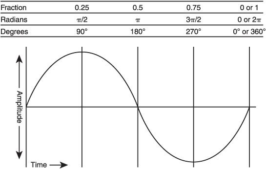
The optional iphs input to oscil controls the starting phase—that is, the point in the stored waveform at which playback will start. This parameter defaults to 0, which is the starting point of the waveform; iphs is expressed as a fraction of a wave cycle, so its value should be set between 0 and 1. The concept is illustrated in Figure 7.1.
It’s often useful to send varying signals rather than constant ones to the xamp and xcps inputs of an oscil. For instance, we can patch the output of an envelope generator into the xamp input. The value of iamp (which might be coming from the score, although in the preceding example it’s set as a constant) is used as the first input to line, which supplies an extemely simple decaying envelope.
  kampenv line iamp, p3, 0
  asig oscil kampenv, kcps, ifn
This is often a convenient way to work, but there are times when we would like the output level of an oscil to remain constant, in which case we would apply the envelope signal using a separate multiplication operation. In the code below, the oscil has a constant output amplitude of 1, and the envelope is applied to the resulting signal using multiplication:
Figure 7.1 Each point in a cyclically repeating waveform has a phase. The phase is defined by the distance between the current point and the starting point of the wave. Phase is sometimes stated in radians (values between 0 and 2À) or in degrees (values between 0 and 360 degrees). In some Csound opcodes, phase is defined, more conveniently, as a number between 0 and 1. Both 0 and 1 correspond to the starting point of the waveform, since the waveform repeats. Values between 0 and 1 (or between 0 and 2À, or between 0 and 360 degrees) correspond to various point on the waveform.
  kampenv line iamp, p3, 0
  asig oscil 1, kcps, ifn
  aout = asig * kampenv
  outs aout, aout
The inputs to oscil can also be used for amplitude or frequency modulation, which will have the effect of altering the shape of the output waveform. To hear this, try replacing the oscil line in the original example with these two lines:
  amod oscil kamp, kcps * 0.5, ifn
  asig oscil amod, kcps, ifn
The output of the first oscil, which is called amod, is being used to control the amplitude of the second oscil. If you try this, you may also want to delete the second line from the example score above, as modulating one sawtooth wave from another tends to sound rather nasty.
A variant of oscil is called oscili. The two are identical except that oscili interpolates between data points in the f-table waveform. Interpolation will produce a smoother output signal. In the early days of Csound, when computers had much less memory, interpolating oscillators were more important. An f-table might be defined with a size of only 128 or 256. Reading the data from such a small table without interpolating tended to produce audible distortion in the sound. Today, memory constraints are all but nonexistent, so an f-table size of 65,536 is just as easy to use. With such a large table, you’re not likely to hear a difference in sound between oscil and oscili. If you’re rendering your finished composition to the hard drive, there’s no reason not to use oscili. But because it’s more computationally intensive, if you’re designing an instrument to be used in real time, you’ll gain a small performance advantage (probably trivial on a modern computer unless you’re generating a lot of signals at once) by using oscil.
![]()
Note A number of opcodes have optional interpolated forms. Usually, if the name of the opcode ends with -i, it interpolates between stored data values, producing a smoother output. The -i versions do linear interpolation. Some opcodes also have a version ending in -3, which does cubic interpolation. Cubic interpolation can produce a cleaner sound, but again, it’s more computationally intensive.
We can also use oscil as an LFO (low-frequency oscillator) to generate modulation signals. For more on this topic, see “LFOs,” later in this chapter. We can even use it as an envelope generator, by setting the frequency value (kcps) to 1/p3. Since p3 always refers to the note’s duration in seconds, 1/p3 will give us exactly one cycle of the oscil waveform during the course of the note. To hear this concept in action, try this example:
  instr 1
  kampenv oscil 0.5, 1/p3, 2
  asig oscil kampenv, 440, 1
  outs asig, asig
  endin

  </CsInstruments>
  <CsScore>

  f1 0 16384 10 4 3 2 1
  f2 0 8192 7 0 200 1 300 0 400 1 500 0 600 1 6192 0

  i1 0 2
  i1 + 3
  i1 + 1
The important thing to notice here is that the control signal kampenv is being generated by an oscil, which is running at k-rate rather than at a-rate. The envelope contour (created in f-table 2 using GEN routine 07) has three quick peaks during the attack and then drops smoothly back to 0. The speed with which the peaks are articulated depends entirely on the length of the note— with slower notes, the attack peaks are spread further apart. If you want attack segments that are always the same length, no matter how long or short the note is, see the section on “Envelopes” later in this chapter.
Other Oscillators
After experimenting with oscil, you may want to look at buzz, gbuzz, and vco.
buzz and gbuzz
buzz and gbuzz are good for creating static tones containing some or many partials. You can process such tones through filters, a standard technique known as subtractive synthesis. Here is a simple example using buzz. As usual in this book, the opening and closing tags in the .csd file have been omitted.
  sr = 44100
  ksmps = 4
  nchnls = 2
  0dbfs = 1

  ; create a sine wave for buzz to use:
  giSine ftgen 0, 0, 8192, 10, 1

  instr 1
  idur = p3
  iamp = p4
  ifrq = p5
  icutoff = 7000
  inumpartials = 35

  asig buzz    1, ifrq, inumpartials, giSine

  ; filter the signal and modulate the cutoff with a simple descending
  ramp:
  kfiltenv line      icutoff, idur, ifrq
  afilt lpf18        asig, kfiltenv, 0.6, 0.1

  kamp linen         iamp, 0.01, idur, 0.1
  afilt = afilt * kamp
  outs afilt, afilt
  endin

  </CsInstruments>
  <CsScore>

  ; play a three-second note at 200Hz with a filter sweep:
  i1 0 3 0.8 200
In this example, buzz produces a signal with 35 partials. The tone is then lowpass-filtered by lpf18.
One limitation of buzz is that all of the partials will be at the same amplitude. In addition, the lowest partial will always be the fundamental. gbuzz is more flexible. Note, however, that gbuzz requires a cosine wave, not a sine wave, as its source material. We can create a cosine wave using GEN 11. The arguments of this GEN routine are slightly different from the arguments for GEN 10, but in this case it hardly matters. Using the example above, substitute the following for the ftgen line:
giCos ftgen 0, 0, 8192, 11, 1
Next, replace the buzz line with this:
asig gbuzz 1, ifrq, inumpartials, 1, 1, giCos
The sound should be exactly the same as before, because this usage of gbuzz sets the lowest partial and the multiplication factor both to 1. But now we can make a few changes. For a tone that emphasizes the upper partials, you might replace 1, 1 in the line above with 5, 1.1. This produces a tone whose lowest partial is the 5 and whose higher partials are progressively louder. (You may find this easier to hear if you get rid of the filter in the example.) Conversely, 1, 0.9 will produce a more muted tone, and 5, 0.9 will produce a tone that sounds a bit bandpass-filtered, as the lowest partials will be gone and the highest partials will be reduced in amplitude.
vco2
To generate a sawtooth or square wave for classic analog synthesis sounds, using vco2 is simple. The default output, a sawtooth, requires no inputs but the amplitude and frequency:
asig vco2 kamp, kfrq
For a square or triangle wave, add a 10 or 12 as a third argument:
asig vco2 kamp, kfrq, 10
The third argument can take other values; see the manual page for a list.
Pulse width modulation of a square wave, an effect common on analog synthesizers, requires only a bit more in the way of setup. Set the imode argument to 2 rather than 10 and then apply a signal (desired values greater than 0 and less than 1) to the kpw argument:
  klfo lfo 0.3, 0.5
  klfo = klfo + 0.5
  asig vco2 kamp, kfrq, 2, klfo
Noise Generators
Random numbers have many uses in computer-generated music. For instance, we might want to fill a table with note pitch values at the start of a performance and let Csound choose the pitches for the table according to some quasi-random algorithm that we devise. Or we might want to add a small random value to the frequency of a vibrato LFO at the start of a note, so that the vibrato will vary slightly from note to note, thus producing a less mechanical sound.
Audio-rate signals containing random numbers are called noise. By mixing noise with other sound sources, we can make more realistic percussion sounds and produce other effects.
For some purposes, such as generating streams of notes, it’s not desirable that the distribution of random numbers be uniform from 0 to some arbitrary value. For example, we might want mostly low numbers and only a few higher ones. Csound provides a variety of random number generators with various features, allowing us to produce weighted random series, random series that are constrained within a specific range (such as between 0 and 10), and so forth.
The precise nature of the weighted curves produced by such opcodes as betarnd, cauchy, and poisson is not well documented in The Canonical Csound Reference Manual (at least, not in the version of the manual released with Csound 5.13—future manuals may contain more information). Fortunately, specific information is readily available online: A search for “cauchy distribution” or “poisson distribution” will turn up articles full of graphs and equations.
To begin our all-too-brief survey of Csound’s random signal sources, let’s look at this instrument:
  instr 1
  seed 0
  ; generate a stream of white noise:
  ahiss rand 0.5
  ; generate a stepped random control signal:
  kstep randomh 500, 5000, 3, 3
  ; use the stepped signal to control filter cutoff:
  aout lpf18 ahiss, kstep, 0.7, 0.5
  outs aout, aout
  endin
The rand opcode, which is used here to generate a stream of white noise, is one of the simpler opcodes in this group. It can produce either an a-rate or a k-rate signal. Here is its prototype:
ares rand xamp [, iseed] [, isel] [, ioffset]
In the example instrument we’re ignoring the optional parameters; we’re giving it only an amplitude argument, 0.5. This assumes 0dbfs=1, as in most of the examples in this book.
The randomh opcode is a little more interesting. It generates random output values and then holds them for some period of time before taking a new random value. In other words, this is a classic analog sample-and-hold—at least, as that term is usually understood. A real sample-and-hold circuit can sample any input signal, not just noise. Here is its prototype of randomh:
kres randomh kmin, kmax, kcps [, imode] [, ifirstval]
The kmin and kmax values limit the minimum and maximum output. The kcps value tells the sample-and-hold how often (how many times per second) to take a new sample. This example uses randomh to control the cutoff frequency of a filter, so it’s set to run at 3 Hz.
The two random signals, ahiss and kstep, are fed into a resonant lowpass filter, lpf18, the first as an audio signal to be filtered, the second as a control signal that controls the filter’s cutoff frequency. The result is step-filtered white noise. To hear this instrument, use a single note in the score, like this:
i1 0 5
This instrument has one other important feature: It uses the seed opcode. Seeding a random number generator is an important concept in computer science. The reason is because computers can’t actually generate numbers at random; their operations are entirely deterministic. Procedures that apparently generate random numbers in a computer are actually clever algorithms that use mathematical formulas to output streams of numbers—streams in which the individual numbers that appear cannot easily be predicted. That is, they’re pseudo-random.
A pseudo-random number generator needs a starting point. The seed value provides this starting point. Csound gives us two ways to use seed. If we give it, as an argument, an integer between 1 and 2^32 (that is, 2 to the 32nd power), then the seeded random number generators will produce the same result every time they’re run. That is, the content of the random number stream will still seem random, but it will be exactly the same each time the music is played. This can be quite useful when you’re generating patterns of notes. If you think your orchestra is doing what you want, but you don’t hear a pattern that pleases you, just change the seed value and play the piece again.
Conversely, if seed is given an argument of 0, the seed value will be taken from the computer’s system clock. This clock will run for years without ever producing the same number, so your pattern of random numbers will be different each time the piece is run.
Some of Csound’s noise sources—specifically, rand, randh, randi, rnd(x), and birnd(x)—are not affected by the seed opcode. The first three have their own private arguments for a seed value, which operate in a similar way; see the manual for details.
Next, let’s use a random number generator to produce a tone with some instability. Using the same score as before (a single note of five seconds or so), try this instrument:
  instr 1
  iSine ftgentmp 0, 0, 8192, 10, 1
  ahiss rand 800
  afilt tonex ahiss, 10
  aosc oscil 0.5, 440 + afilt, iSine
  outs aosc, aosc
  endin
The first line uses ftgentmp to fill a table with a sine wave. The table number, iSine, is passed to oscil to be used as a waveform. As before, we’re using rand to produce white noise, but the amplitude (800) is higher than before. The noise is filtered using tonex so that only very low frequencies remain. The filtered noise is used to modulate the frequency of oscil. The result is a tone whose frequency wobbles up and down in a random way, but only slightly.
Experiment with different arguments to rand and tonex and listen to the result. If you increase the amount of pitch wobble (perhaps to 440 + afilt * 5), you’ll discover that the output of rand is very non-random indeed: It loops through a cycle about once per second. Since we’re creating an audio-rate signal using rand, it’s a fair inference that it puts out on the order of 44,000 different numerical values before repeating. This is good enough in many situations, but perhaps not in this instrument. So let’s try something different.
Replace the rand and tonex lines with a call to randomi and edit the oscil line, as shown below:
  kwobble randomi -15, 15, 15, 2
  aosc oscil 0.5, 440 + kwobble, iSine
The randomi opcode produces a sort of zigzag output. Periodically, it generates a new random number and then ramps smoothly up or down from the previous value to the new one. In the code above, it’s selecting a new value 15 times per second, and the value will be somewhere between −15 and 15. Now there is no detectable pattern to the pitch wobble.
For our final example of randomness, we’re going to let the random opcode choose what note an instrument will play. We’ll generate a random number between 0 and 1 and then choose the oscillator frequency based on the number. Csound lacks a switch statement (a convenient bit of syntax in computer programming), so we have to use a series of else/then/if statements to select a pitch. This makes the instrument look a little more complex than it is. The score also takes up more lines: To make the effect of the randomness clearer, we’ll play a bunch of notes.
To lead into the next section of Csound Power!, I’ve employed a foscil opcode in this example. Also pressed into service is the useful cpspch opcode, which will be discussed in the section on “Pitch Converters,” later in this chapter. Here is the bulk of the .csd file (leaving off the <...> tags at the beginning and end):
  sr = 44100
  ksmps = 4
  nchnls = 2
  0dbfs = 1
  seed 0

  instr 1
  iSine ftgentmp 0, 0, 8192, 10, 1
  ; generate a random number between 0 and 1:
  iRand random 0, 1

  ; choose a definite pitch for the note, basing the choice on the random
  number:
  if iRand < 0.2 then
        ifreq = cpspch (7.0)
  elseif iRand < 0.4 then
        ifreq = cpspch (7.04)
  elseif iRand < 0.6 then
        ifreq = cpspch (7.07)
  elseif iRand < 0.8 then
        ifreq = cpspch (7.09)
  else
        ifreq = cpspch (8.0)
  endif

  kenv line 0.5, p3, 0
  aosc foscil kenv, ifreq, 1, 1, 5 * kenv, iSine
  outs aosc, aosc
  endin

  </CsInstruments>
  <CsScore>

  i1 0 0.2
  i1 +
  i1 +
  i1 +
  i1 +
  i1 +
  i1 +
  i1 +
  i1 +
  i1 +
  i1 +
  i1 +
  i1 +
  i1 +
  i1 +
This example will play 15 notes selected at random from a pentatonic scale in C major.
FM Synthesis
The techniques of FM (frequency modulation) synthesis were first developed in the 1970s, primarily by John Chowning at Stanford University. FM was first popularized in the Yamaha DX7 synthesizer, which debuted in 1983. Though by now the DX7 is completely obsolete, it remains one of the best-selling and most-often-heard synthesizers of all time, and FM synthesis remains a very viable way to generate complex and interesting tones. Many currently available synthesizers, especially software plug-ins, have facilities for FM synthesis, usually in conjunction with other techniques.
In FM synthesis, the frequency of one oscillator (called the carrier) is modulated by the signal from another oscillator (called the modulator). What the listener hears is normally the signal coming from the carrier. Quite often, both oscillators use sine waves as their source waveform, but in fact any waveform can be used. If the modulator is running in the sub-audio frequency range (below about 20 Hz), the result of frequency modulation is vibrato. When the modulator’s frequency rises into the audio range, however, something very interesting happens: Instead of hearing the frequency changes of the carrier as pitch fluctuations, we hear them as a change in the tone color of the carrier.
Several very decent tutorials on FM are available online, so there’s no need to recapitulate them here. Instead, let’s dive straight in and start making some sounds.
FM Using foscil
Csound gives us several different ways to implement FM. Perhaps the easiest to use is the foscil opcode. This opcode models a pair of oscillators configured as a carrier and a modulator, producing a single output signal from the carrier. Here is the prototype of foscil:
ares foscil xamp, kcps, xcar, xmod, kndx, ifn [, iphs]
If you’ve read the section earlier in this chapter on oscil, you’ll know that ares is the output audio signal, xamp is the input for the amplitude level, kcps the input for the frequency, and ifn the number of the f-table to use to generate the waveform. In FM, this should usually be a sine wave. Other waves can be used, but they tend to generate quite a lot of overtones, so aliasing distortion is likely. The optional iphs parameter is for setting the start phase of the signal and can almost always be ignored.
The new parameters are xcar, xmod, and kndx. The first two are used for setting the frequencies of the carrier and modulator relative to the value in kcps. In the example below, we’ll set them both to 1. These settings will give foscil a warm, sawtooth-like tone.
The kndx input controls the amount of modulator signal that is applied to the carrier. As this value rises, the signal will have more and stronger partials. Because it’s a k-rate input, we can easily send it a signal coming from an envelope generator. As the envelope level falls, the output of foscil will have fewer partials. Depending on the values of xcar and xmod, this may or may not sound similar to an envelope generator lowering the cutoff frequency of a lowpass filter. When the value of kndx falls to zero, there will be no frequency modulation, so only the bare tone of the carrier oscillator will be heard.
Partials, Overtones, and Harmonics Musicians tend to use the words “overtones” and “harmonics” when describing tone color. The term “partials” is heard less often, but in some cases it’s more correct.
The underlying mathematical theory is that any periodic waveform (that is, anything that’s not noise) can be analyzed as a group of one or more sine waves, each having its own frequency, amplitude, and phase. When you pluck a guitar string, for instance, your ear interprets the sound as a single tone, but the tone is actually a composite: It contains sound energy at many different frequencies. That is, it comprises a number of partials.
The terms “overtones” and “harmonics” contain a hidden assumption, which is that the frequencies of the various sine-wave partials have a simple mathematical relationship to one another. Specifically, they’re all whole-number multiples of some base frequency, which is called the fundamental. This is a fairly good (though imperfect) assumption with respect to the sound of plucked strings and vibrating columns of air. If the guitar string is tuned to 100 Hz, the tone will contain energy at 200 Hz, 300 Hz, 400 Hz, and so forth.
But in some situations, the sine-wave components of a tone don’t have this simple mathematical relationship. A bell, for instance, vibrates in a more complex way than a string. The sine waves in the sound of a bell can only be termed partials, because they’re not overtones or harmonics. Likewise, in digital synthesis, it’s easy to produce tones whose sine-wave components are not related by ratios that can be described using whole numbers.
To start exploring FM synthesis, create this simple .csd file (as usual, the tags at the beginning and end of the file have been omitted in the example, to save space).
  sr = 44100
  ksmps = 4
  nchnls = 2
  0dbfs = 1

  giSine ftgen 0, 0, 8192, 10, 1

  instr 1
  kampenv line 0.5, p3, 0
  aosc foscil kampenv, 110, 1, 1, 5, giSine
  outs aosc, aosc
  endin

  </CsInstruments>
  <CsScore>
  i1 0 2
Try replacing the two 1’s in the foscil line with other values. Start with integers, and also try some decimal values, such as 1.37 for either xcar or xmod. You’ll find that each combination of numbers creates a distinct tone color.
Try increasing the value for kndx (5 in the example). This will add partials to the tone. Another way to add partials is to edit the ftgen line in the header. If you look up the prototype for GEN 10, which is being used here, you’ll see that the number or numbers at the end of the line add more sine wave overtones to the fundamental stored in the table. You can add several overtones and give them various strengths, like this:
giSine ftgen 0, 0, 8192, 10, 1, 2, 3
By patching an LFO or envelope generator signal into the kndx input of foscil, we can shape the tone. Change the instrument code so that it looks like this:
  instr 1
  kampenv line 0.5, p3, 0
  indxmax = 10
  kindex linseg indxmax, 0.2, 1, 0.1, indxmax * 0.8, p3 - 0.3, 0
  aosc foscil kampenv, 110, 1, 1, kindex, giSine
  outs aosc, aosc
  endin
The FM index envelope (called kindex above) is generated by a linseg envelope generator. To make it easier to edit the envelope and thereby alter the brightness of the tone, the value indxmax has been pulled out as a separate i-rate variable. In a more fully developed instrument, indxmax would probably be controlled from the score, or perhaps from a velocity value being transmitted by a MIDI keyboard.
FM Using phasor and table
The foscil opcode is convenient but limited. It implements a single carrier/modulator pair; in FM parlance this is called two-operator FM. There are times when we may want to have two modulators modulate the frequency of a single carrier, or have a single modulator affect two carriers at once. For this, we need a more flexible instrument design. The key to developing more flexible FM synthesis lies in the use of the phasor and table opcodes.
A phasor is a special type of oscillator. It produces a ramp that moves upward from 0 to 1 and then repeats. Essentially, it produces a rising sawtooth wave, but you probably wouldn’t want to listen to it directly, as the sound would include aliasing. A phasor is normally paired with an opcode that reads the data from an f-table. The most basic form of this opcode is table. In the code example below, I’ve used tablei instead; the -i on the end of the name indicates that this is an interpolating opcode, which can produce a slightly smoother output.
  instr 1
  ; create a sine wave:
  iSine ftgentmp 0, 0, 8192, 10, 1
  ; initial settings:
  iamp = 0.5
  ifreq = 110
  index = 2
  imodfactor = 1
  icarfactor = 1

  ; envelopes:
  kampenv line iamp, p3, 0
  kindex line index, p3, 0
  ; tone generation:
  amodsig oscili kindex, ifreq * imodfactor, iSine
  acarphas phasor ifreq * icarfactor
  asig tablei acarphas + amodsig, iSine, 1, 0, 1

  ; output:
  aout = asig * kampenv
  outs aout, aout
  endin
The comments in the example code above may help you see what’s going on. The new functionality is in the tone generation section. Here we create a modulator using oscili and a carrier using a phasor/tablei pair. The sine wave in the table (created by ftgentmp) is read at a frequency specified by the addition of acarphas (the output of the phasor) and amodsig (the output of the modulator).
To change the relative tuning of the carrier and modulator, enter other values for imodfactor and icarfactor.
If you play this instrument with a reasonably long note from the score—five seconds or so— you’ll hear that it has a rather rich sound. Acoustic energy is moving from one partial to another during the tone. In fact, what we’re doing now is not technically FM synthesis; it’s phase modulation synthesis. Phase modulation has some advantages with more complex patches. For instance, it’s more stable when we add a feedback loop, in which a portion of the carrier signal is used to modulate the carrier itself. This type of feedback, which produces a brighter sound, was implemented in the DX7.
Here is the tone generation portion of the instrument above, altered to add some feedback. Note the use of init. In order to include asig among the arguments to tablei, we have to initialize it. When we’ve done this, the compiler knows that it exists, so we won’t get an error message when we run the instrument. I found values that I liked for the new linseg (the feedback amount envelope) by trial and error. This envelope sounds good to me with a tone that lasts for about five seconds. (In the DX7, if memory serves, the amount of feedback was not controllable by an envelope.)
  ; tone generation:
  kfeedback linseg 0.2, 0.5, 0.1, 1.5, 0
  asig init 0
  asig = asig * kfeedback
  amodsig oscili kindex, ifreq * imodfactor, iSine
  acarphas phasor ifreq * icarfactor
  asig tablei acarphas + amodsig + asig, iSine, 1, 0, 1
Granular Synthesis
The theory of granular synthesis is not especially complicated, but putting the theory into practice can lead to a certain amount of confusion and frustration. To see why, take a quick look at the prototype for the granule opcode:
  ares granule xamp, ivoice, iratio, imode, ithd, ifn, ipshift, igskip,
    igskip_os, ilength, kgap, igap_os, kgsize, igsize_os, iatt, idec
    [, iseed] [, ipitch1] [, ipitch2] [, ipitch3] [, ipitch4] [, ifnenv]
That’s 16 required inputs, plus half a dozen more that are optional—and no, I’m not going to pause to explain each and every one of them here. Fortunately, Csound includes several granular synthesis opcodes that are easier to use than granule. Even so, as you explore the powerful resources of granular synthesis you should plan to devote a few hours to experimentation.
In granular synthesis, a sustained sound is built up by stringing together hundreds or thousands of short “sound grains.” (See, I told you the theory wasn’t complex. That’s really all there is to it.) The basic parameters the sound designer specifies include:
![]() The source waveform used in the grains.
The source waveform used in the grains.
![]() The starting points of the grains within the source.
The starting points of the grains within the source.
![]() The lengths of the grains.
The lengths of the grains.
![]() The pitches of the grains.
The pitches of the grains.
![]() The amplitude envelope used to shape the grains.
The amplitude envelope used to shape the grains.
![]() The amount of time that separates one grain from the next.
The amount of time that separates one grain from the next.
Specifying all of these parameters for each grain individually would be a monstrous task. Fortunately, Csound provides several granular synthesis opcodes that take care of the details. The sound designer need only provide one value for each of them, or a k-rate input to modulate them during the course of a long tone, and Csound takes care of the messy details.
It’s possible to do something very similar yourself, using an event opcode in some sort of loop to start notes on your own instrument, which will then play a grain. This approach gives you a little more control over the grains; you could filter them in various ways, for instance, by employing a filter in the instrument that is playing them. An example of this technique is given at the end of this section. But the detailed, hands-on approach of using event is not always needed.
Let’s look at the control parameters one at a time.
The source waveform used in granular synthesis is often a sampled (digitally recorded) sound—a file on your computer’s hard drive. Sampled drum loops and spoken vocal phrases are good— anything with some variety in it. A single sampled note would probably be less interesting. Usually a monaural file will be needed; if you want to try using a stereo file as a source for granular synthesis, you’ll probably want to load it into an audio editor such as Audacity and create a mono version. Alternatively, Csound lets you load each channel of a stereo file into a different table, so you could apply granular processes to the left and right channels independently. Because many granular processes involve a bit of randomization, however, it’s not likely the left and right channels will stay in sync.
With a source waveform of reasonable length, the starting point for each new grain can be at a different point in the source. The starting points could proceed forward through the source, or backward, or be selected at random.
Grains are typically between 1ms and 50ms in length. As the grains become longer, the nature of the source material can be heard more easily. Using a drum loop as a source for granular synthesis and setting a larger grain size can give you a comically mangled, staggering drum track, in which the individual drum sounds are heard clearly but all rhythmic coherence is lost.
The grains can be played back at their original pitch—that is, the output rate can be the same as the rate at which the source digital recording was originally made. Or they can be played back faster or slower than the original pitch. Changing the pitch of the grains is a way of altering the pitch of a sampled sound without affecting its length.
The grain’s amplitude envelope is usually defined with an attack time and a decay time. During the attack time, the envelope will rise from zero to its maximum amplitude; it will then hold that amplitude constant until the decay time starts. During the decay time, the envelope will fall back to zero (see Figure 7.2). This scheme is a bit simpler than the classic ADSR envelope found in traditional synthesizers, in that the sustain level is always 100%. In the prototype for granule shown above, the attack and decay time of the grain envelope can be set using the iatk and idec parameters. (For details on how these inputs work, consult the granule page in The Canonical Csound Reference Manual.) Another option is to get the envelope from a function table. This approach is used in the grain opcode.
Figure 7.2 The amplitude envelope of a sound grain is usually defined by its attack and decay time. In some implementations, you may also be able to select a curve type for the attack and decay.

If there’s a silent gap between the end of one grain and the beginning of the next, the sound will have a stuttering quality. The stuttering may be so fast, however, that it’s audible only as a certain roughness in the tone or as a low frequency. On the other hand, the time between the end of one grain and the start of the next might be negative. Another way of stating this is that the grain length is greater than the difference in start times between one grain and the next. In this situation, the grains will overlap. If they overlap, the sound will be smoother and richer.
The grain Opcode
A good way to get started with granular synthesis is to copy the example code for grain in the manual, paste it into a CsoundQt file, and then play around with it. The source soundfile used in this example, beats.wav, is installed with Csound. You can use it as the source with this example by copying it into the directory you have set as SFDIR in the Environment tab of the CsoundQt Configuration box.
Here is the prototype for grain:
  ares grain xamp, xpitch, xdens, kampoff, kpitchoff, kgdur, igfn,
    iwfn, imgdur [, igrnd]
As usual, the backslash character at the end of the line is Csound’s shorthand for continuing a long line of code without going off the right edge of the window.
The xamp, xpitch, and xdens inputs are easy to understand: They control the amplitude, pitch, and density of the grains. (The density value is in grains per second.) More interestingly, this opcode has three internal sources of controlled randomness. The value for kampoff determines the amount of random variation in the amplitude. When this parameter is 0, the value in xamp will be used directly, but when kampoff is not 0, the maximum amplitude will be xamp + kampoff, and the minimum will be xamp – kampoff. The same consideration applies to xpitch and kpitchoff: When kpitchoff is not 0, the actual output pitch of a grain will be randomly higher or lower than the value in xpitch. Finally, the point within the source sound file (igfn) where the grains will start their playback can be randomly chosen (if igrnd is 0) or at the beginning of the file (if igrnd is not 0). Because of this built-in randomness, the example in the manual produces two entirely different output audio streams from two grain lines of code, one being sent to the left output channel and the other to the right, even though the lines themselves are identical.
After copying the example code from the manual into your own .csd, you might try these experiments:
![]() Increase the end value in the line that creates kpitch to ibasefreq * 4. As the output of the line opcode ramps up, the pitches of the grains will rise.
Increase the end value in the line that creates kpitch to ibasefreq * 4. As the output of the line opcode ramps up, the pitches of the grains will rise.
![]() Lower the starting and ending values for kdens from 600 and 100 to 6 and 10. This will give you a much more sparse scattering of grains.
Lower the starting and ending values for kdens from 600 and 100 to 6 and 10. This will give you a much more sparse scattering of grains.
![]() Try different source audio files. If your file is longer than beats.wav, you may want to increase the size of f10 to some larger power of two.
Try different source audio files. If your file is longer than beats.wav, you may want to increase the size of f10 to some larger power of two.
Granular Synthesis by Hand
Next, let’s look at an orchestra that uses event to generate grains manually. (For more on event, see “Creating Score Events during Performance,” later in this chapter.) The grain-playing instrument has a sine wave as its source, but you could easily substitute any other type of tone. Adding more p-fields (perhaps for filter cutoff, varying decay time, or source waveform) and filling them with either random numbers or values that ramp up or down would be just as easy.
  sr = 44100
  ksmps = 4
  nchnls = 2
  0dbfs = 1
  giSine ftgen 0, 0, 8192, 10, 1

  instr 1; play a sine wave
  iatk = 0.01
  idec = 0.01
  isus = p3 - iatk
  iamp = p4
  ifreq = p5
  ipan = p6

  ifreqrampend random 0.7, 1.3
  kfreq line ifreq, p3, ifreq * ifreqrampend

  kampenv linsegr 0, iatk, iamp, isus, iamp, idec, 0
  asig oscil kampenv, kfreq, giSine

  aoutL, aoutR pan2 asig, ipan
  outs aoutL, aoutR
  endin

  instr 11; a grain generator
  kamp random 0.15, 0.3
  kfreq random 300, 800
  kpan random 0, 1
  kdur random 0.05, 0.15
  ktimerand random -3, 3
  ktrig metro 20 + ktimerand
  if ktrig == 1 then
    event “i”, 1, 0, kdur, kamp, kfreq, kpan
  endif
  endin

  </CsInstruments>
  <CsScore>
  i11 0 5
  e 5.2
As usual, I’ve omitted the opening and closing tags in the .csd file. The e 5.2 line at the end of the score extends the length of the score slightly, in order to allow the last grain to finish playing. Without this line, you may hear a click when the tone stops.
The grains are generated at a time determined by the metro opcode. The tempo of this is being randomized somewhat, so that the grains don’t have a regular rhythm.
The grain envelope is generated by linsegr. This opcode has a release segment, so the actual grain length is idec longer than p3. It’s a typical rise-sustain-decay envelope. To make the sound a little more interesting, I’ve given the sine-wave instrument its own random-depth pitch envelope, which can rise or fall somewhat during the grain.
Formant Synthesis
Formants are resonant regions within the frequency spectrum. The term “formant” is most often associated with the vowel sounds produced by the human voice. The human larynx (vocal cords) produces a raw tone that is somewhat like a sawtooth wave: It’s rich in overtones. The overtones coming from the vocal cords pass through the resonant cavities of the mouth and sinuses, and these resonant cavities emphasize certain overtones while attenuating others. The human ear and brain are exquisitely sensitive to the differences in tone color that can be produced by changing the shape of the mouth, and for obvious reasons: Without such sensitivity, spoken language would be harder to understand. As a result, electronic tones that have a vocal quality can be surprisingly evocative.
As the description above may suggest, one way to produce this type of tone color is by starting with a broad-band tone, such as a sawtooth wave or white noise, and passing it through a set of parallel bandpass filters. A bank of such filters is sometimes referred to as a formant filter.
Csound gives us a second way to synthesize vocal tones. We can build them up additively using granular synthesis. The opcodes that are most often used for this purpose are fof, fof2, and fog.
These opcodes have enough input parameters that they can be rather intimidating. Here is the prototype for fof:
  ares fof xamp, xfund, xform, koct, kband, kris, kdur, kdec, iolaps,
    ifna, ifnb, itotdur [, iphs] [, ifmode] [, iskip]
For details on the meanings of the arguments, consult the manual page on fof. The first two arguments, xamp and xfund, aren’t hard to understand: They’re the amplitude of the output signal and the frequency of the fundamental tone. xform and xband are used to control the formant frequency and bandwidth.
To get you started, scroll down to the lower end of the left pane in the HTML manual. You’ll see links to several Appendices. Appendix D lists the formant values for common vowels. (Note that most vowel sounds in English are actually diphthongs. That is, they’re produced by gliding from one vowel sound to another. Many languages employ pure vowel sounds rather than diphthongs, and the data in Appendix D produces pure vowel sounds.)
The values for kris, kdur, and kdec control the rise time, duration, and decay time of individual grains within the tone. ifna and ifnb are the numbers of function tables; for vocal synthesis, the first table is normally a sine wave. The second table contains a rise shape, which is applied to the grain over the time defined by kris and kdec.
The value koct operates backwards from what you might expect. A value of 0 produces a “normal” vocal tone. As koct increases, the fundamental drops. An increase from 0 to 1 drops the fundamental by an octave (hence the name) while leaving the formants where they are.
The best way to learn to use these opcodes is probably to start with a working code example and then start varying it to see how the sound changes. The example below generates the sound of a vocal “ah” tone using four instances of fof, each of which generates one formant. As usual in this book, the opening and closing tags in the .csd file have been omitted.
  sr = 44100
  ksmps = 128
  nchnls = 2
  0dbfs = 1

  instr 1; plays a vocal tone consisting of four formants
  idur = p3
  iamp = p4
  ifund = p5
  ioct = p6

  iamp1 = ampdb(0) * iamp
  iamp2 = ampdb(-4) * iamp
  iamp3 = ampdb(-12) * iamp
  iamp4 = ampdb(-18) * iamp
  iatk1 = 0.1
  iatk2 = 0.12
  iatk3 = 0.14
  iatk4 = 0.16

  irel1 = 0.2
  irel2 = 0.24
  irel3 = 0.28
  irel4 = 0.32

  iformfrq1 = 800
  iformfrq2 = 1150
  iformfrq3 = 2800
  iformfrq4 = 3500

  ibandw1 = 80
  ibandw2 = 90
  ibandw3 = 120
  ibandw4 = 130

  ; we’ll leave these at their default values:
  kris init 0.003
  kdur init 0.02
  kdec init 0.007
  iolaps = 14850

  ifna = 1
  ifnb = 2

  ; now for a little fun with LFOs:
  iformlforate = 4.0
  iformlfoamt = 30
  iamplforate = 2
  iamplfoamt = 0.03
  kformlfo oscil iformlfoamt, iformlforate, 1
  kamplfo oscil iamplfoamt, iamplforate, 1

  kformfrq1 = iformfrq1 + kformlfo
  kformfrq2 = iformfrq2 + kformlfo
  kformfrq3 = iformfrq3 + kformlfo
  kformfrq4 = iformfrq4 + kformlfo
  kenv1 expseg 0.0001, iatk1, iamp1, (idur - (iatk1 + irel1)),  iamp1, irel1, 0.0001
  kenv2 expseg 0.0001, iatk2, iamp2, (idur - (iatk2 + irel2)),  iamp2, irel2, 0.0001
  kenv3 expseg 0.0001, iatk3, iamp3, (idur - (iatk3 + irel3)),  iamp3, irel3, 0.0001
  kenv4 expseg 0.0001, iatk4, iamp4, (idur - (iatk4 + irel4)),  iamp4, irel4, 0.0001

  kamp1 = (1 + kamplfo) * kenv1
  kamp2 = (1 + kamplfo) * kenv2
  kamp3 = (1 + kamplfo) * kenv3
  kamp4 = (1 + kamplfo) * kenv4

  a1 fof kamp1, ifund, kformfrq1, ioct, ibandw1, kris, kdur, kdec,
    iolaps, ifna, ifnb, idur
  a2 fof kamp2, ifund, kformfrq2, ioct, ibandw2, kris, kdur, kdec,
    iolaps, ifna, ifnb, idur
  a3 fof kamp3, ifund, kformfrq3, ioct, ibandw3, kris, kdur, kdec,
    iolaps, ifna, ifnb, idur
  a4 fof kamp4, ifund, kformfrq3, ioct, ibandw4, kris, kdur, kdec,
    iolaps, ifna, ifnb, idur

  asig = a1 + a2 + a3 + a4
    outs asig, asig
  endin
  </CsInstruments>
  <CsScore>

  ; a sine wave:
  f1 0 8192 10 1
  ; a curve for shaping the grains:
  f2 0 1024 19 0.5 0.5 270 0.5

  ; play three notes:
  i1 0 2 0.2 250 0
  i1 2.1 2 0.1 350 0
  i1 4.2 3 0.2 350 2
  e
This example produces three stationary tones with a bit of vibrato and tremolo. Because each formant has its own overall attack and release time (not to be confused with the kris and kdec values for the individual grains), the tone has a bit of shape. But much more can be done with this example. The code example for fof in the manual, for instance, uses line opcodes to glide the formant frequencies, amplitudes, and bandwidths during the course of a single note, so that the vocal tone shifts from one vowel to another. For more realistic vocal synthesis, you may want to vary the speed and depth of the LFOs or glide smoothly from one pitch to another. And of course, many combinations of formants produce vowel-like tones that are not possible with the human vocal tract, so singing aliens are a distinct possibility.
Sample Playback
Csound has a number of opcodes with which you can play back audio samples stored on your hard drive. Normally these samples will be in the form of .WAV or AIFF files. In addition, a whole family of opcodes (the so-called Fluid opcodes) is available for playing files in the popular SoundFont format. We’ll have more to say about the Fluid opcodes below.
Before playing a .WAV or AIFF file, you’ll need to load it into an f-table. This is done using GEN 01. One potentially tricky point about GEN 01 is that it expects you to tell it the size of the file in samples. You may not know this. You can enter a 0 as this parameter and let Csound figure it out, but if you do so, you may have trouble further on down the line, as the table opcode doesn’t like deferred-size tables.
To find the size of a file, you can start with a deferred-size table (setting size to 0 in the GEN routine), use the tableng opcode to determine the size, and then use print to print the value out to the Console:
  giSample ftgen 0, 0, 0, 1, “gtrA4.aiff”, 0, 0, 0
  instr 1
  ilen tableng giSample
  print ilen
  endin
When I played a short score that triggered instr 1, I learned that my file was 168,020 samples long. Normally, a GEN routine needs to see a power of 2 or a power-of-2-plus-1 as its size, but you can override this by setting a negative value for size, so I replaced my ftgen line with this:
giSample ftgen 0, 0, -168020, 1, “gtrA4.aiff”, 0, 0, 0
Once you’ve gone through these steps, you’ll be ready to try sample playback.
Sample Playback Using table
The simplest way to play a sample uses the table opcode. Starting with the monaural waveform loaded into the giSample table as shown above, the instrument below will play the sample exactly once, at its original pitch. It will play the sample from start to end, no matter how long or short it is, and no matter how long or short the score event triggering the instrument may be:
  instr 1
  iamp = p4
  ilen tableng giSample
  p3 = ilen/sr
  aphas phasor 1/p3
  aphas = aphas * ilen
  asig table aphas, giSample
  asig = asig * iamp
  outs asig, asig
  endin
This instrument gets the length of the sample using tableng and then resets p3 (the length of the score event) to the length divided by the sample rate at which the orchestra is playing. A phasor then creates a ramp that moves from 0 to 1 exactly once during the (revised) length of the note. This phase value is multiplied by the sample length, so that the table opcode can sweep through the entire table exactly once during the note.
Starting from this template, you should find it fairly easy to play the sample faster or slower, to repeat it in a loop, or to start at a later point than the beginning of the sample. For instance, if you want to play the sample an octave lower (in which case it will last twice as long), substitute this line:
p3 = (ilen/sr) * 2
However, Csound provides some tools to make such modifications easier.
Using loscil
When using loscil, we can skip the messy calculations in the example above. The following instrument is much simpler. If all we want to do is play a sample at its original pitch, we’ll get the same result:
  instr 1
  iamp = p4
  ilen tableng giSample
  p3 = ilen/sr
  asig loscil iamp, 1, giSample, 1, 0
  outs asig, asig
  endin
Here, I’ve taken advantage of the ability of loscil to figure out the sample’s pitch. I’ve set the arguments for kcps and ibas both to 1. I also set imod to 0 to tell loscil that I didn’t want a loop. But much more can be done with loscil. For reference, here is its prototype:
  ar1 [,ar2] loscil xamp, kcps, ifn [, ibas] [, imod1] [, ibeg1] [, iend1]
    [, imod2] [, ibeg2] [, iend2]
You’ll find several examples illustrating the use of loscil in Chapter 3. Reading the manual will provide details on the meanings of the arguments shown in the prototype. Two or three points may be worth mentioning. First, loscil will work with either mono or stereo soundfiles. Second, it always starts playback from the beginning of the file—it doesn’t provide a way to skip the beginning of the file. If you want to start playback at some point after the beginning of the file, you’ll want to adapt the code shown earlier that uses phasor and table.
Third, with loscil you can specify both sustain and release loops. The release loop makes use of the same mechanism as envelope generators with the -r suffix, such as linsegr. If one of these is included in the instrument, then loscil will finish the sustain loop and move on to the release loop when the normal duration of the note (set by p3) is finished and the release segment (the final time value of the -r envelope) begins. Here’s an example. It mangles a sampled stereo drum pattern by interrupting the loop with a short back-and-forth loop and also introducing a pitch envelope. The length of the entire sample (298,141 sample words) was determined using the technique discussed earlier in this section, using tableng and print.
  giSample ftgen 0, 0, -298141, 1, “Drumloop 01.wav”, 0, 0, 0
  instr 1
  idur = p3
  iamp = p4
  iatk = 0.005
  isus = idur - iatk
  irel = 5
  kamp linsegr 0, iatk, iamp, isus, iamp, irel, 0
  kfrq linseg 1, iatk, 1.2, isus, 0.8, irel, 2
  aL, aR loscil kamp, kfrq, giSample, 1, 2, 10000, 18000, 2, 39000, 46000
  outs aL, aR
  endin
Using flooper
If you don’t need both sustain and release loops, flooper may be the tool for the job. Its prototype is:
asig flooper kamp, kpitch, istart, idur, ifad, ifn
The value of kpitch is interpreted as a multiplier of the base frequency of the loop; it can be negative for reverse playback. The other parameters specify the start point of the playback loop, the loop’s duration, the crossfade time, and the f-table number.
Crossfading between the end of a loop and the start of the next play-through of the loop has been a standard technique of sampling since the 1980s. It isn’t always needed with drum loops, where a clearly articulated rhythm is preferred, but can work very well to smooth out loops of sustaining sounds.
![]()
Smooth Loop Strategies When an audio recording (a sample) is played back over and over in a looped fashion, the playback mechanism (such as a Csound opcode) jumps from the end of the loop back to the beginning. If the value of the last data word at the end of the loop is not the same as the value of the first data word at the beginning of the loop, you’ll hear a click.
If both the end of the loop and the beginning are on zero-crossings—points where the waveform crosses from a positive value to a negative value or vice versa—there won’t be a click. In fact, the loop start and end points can be at any value, as long as the two values are the same, but for technical reasons, some early samplers required that the loop points be at a zero-crossing, so setting loop points at zero-crossings has become standard practice.
Another technique that avoids clicks is back-and-forth looping. The loop is played forward until the end point is reached, then played backward until the start point is reached, then played forward again, and so on. In this situation the start point is never directly joined to the end point, so there’s no click.
A third method is to crossfade between the data at the end of the loop and the data at the start.
flooper operates in mono, so if we want to use it to play a stereo sample, we have to create two separate f-tables using GEN 01. One table will contain the left-channel data and the other table the right-channel data. This is done by setting the channel argument (the final argument) to GEN 01 to either 1 (for the left channel) or 2 (for the right channel). During playback, the two channels don’t have to stay in sync; the left and right channel loops can split apart if desired.
The start, duration, and crossfade time of flooper are set in seconds. The crossfade must be shorter than the duration of the loop.
Using diskin2
All of the sample playback methods discussed so far in this section require that the audio data be loaded into RAM before (or during) playback. Given the amount of RAM available in today’s computers, this may not seem to be a problem, but due to the way Csound uses floating-point arithmetic, the upper limit of RAM-based audio is about a minute per sound. (You can load many sound samples into RAM, of course.) In order to play single sounds that are longer than a minute, you’ll need to stream audio directly from a hard disk file using the diskin2 opcode.
diskin2 provides several options, including transposing the audio up or down in pitch and playing it backwards, but the basic version could hardly be easier to use:
  instr 1
  aL, aR diskin2 “finalMix.wav”, 1
  outs aL, aR
  endin
The Fluid Opcodes
SoundFonts are a data format for music synthesis that was developed by E-MU Systems and Creative Labs in the early 1990s. SoundFonts are instrument definitions in which samples are mapped to a MIDI keyboard, often with other features such as envelopes and sample loop points built into the SoundFont. Given that this format was developed for consumer-grade devices, primarily PC soundcards, it may seem odd to want to use SoundFonts in a high-quality system optimized for experimental sound programming—but if you want to use SoundFonts in Csound you can do it, using the Fluid opcodes. You might want to do this if you have a SoundFont that you’re fond of and want to use in a piece of music, or for satirical purposes.
SoundFonts of various kinds are available for download from the Internet, some of them free and some as commercial products. If you’re using a recent installation of Csound for Windows, you’ll find the file sf_GMbank.sf2 in the Samples directory of your Csound directory; if you’re running Mac OS or Linux and want to use this file, post a message to the Csound mailing list, and probably somebody will be willing to send it to you. This 4-MB file includes a full set of General MIDI sounds.
To use a SoundFont in Csound, you need to take five steps. The first three would normally be done in the orchestra header, the final two in one or more instruments.
1. Activate the FluidSynth engine using fluidEngine.
2. Load a SoundFont file using fluidLoad.
3. Tell the engine what sound within the file you want to play by passing a specific bank and preset number to fluidProgramSelect.
4. Play one or more notes on the sound using fluidNote.
5. Capture the output sound stream using fluidOut and send it to Csound’s output.
Some of these opcodes have features we won’t discuss here; they’re explained in the manual. Instead, we’ll jump straight to a code example that uses them to play a little music. Before we do that, though, we need to clear up one question.
A single SoundFont file can contain numerous sounds. The sf_GMbank.sf2 file, in fact, contains a couple of hundred. In Step 3, you’ll be choosing a particular sound by bank and preset number. So how do you know what’s available in the file? The solution is to pass a non-zero number to fluidLoad as the optional ilistpresets argument. This will cause the entire contents of the file to be listed to the Output Console, complete with sound names and their associated bank and preset numbers. Scroll up in the Console pane in CsoundQt (or in the terminal, if you’re running Csound from the command line) to view the list.
The example below instantiates a FluidSynth engine and selects presets for it on channels 1 and 2, in order to play two different GM sounds. The SoundFont file can be specified using a complete directory structure from the root of your hard drive, or the file can be stored in the SSDIR you have chosen.
  sr = 44100
  ksmps = 4
  nchnls = 2
  0dbfs = 1

  ; start an engine:
  giEngine fluidEngine

  ; load the GM SoundFont bank into the engine:
  giSFnum fluidLoad “sf_GMbank.sf2”, giEngine, 1

  ; select active sounds for two channels (bank 0, preset 0 and bank 0,
  ; preset 83):
  fluidProgramSelect giEngine, 1, giSFnum, 0, 0
  fluidProgramSelect giEngine, 2, giSFnum, 0, 83

  instr 1, 2           ; play a note, using p1 to choose a channel:
  ichan = p1
  inote = p4
  ivel = p5
  fluidNote giEngine, ichan, inote, ivel
  endin

  instr 99              ; capture the stereo output signal
                        ; and send it to Csound’s output:

  iamp = p4
  asigL, asigR fluidOut giEngine
  asigL = asigL * iamp
  asigR = asigR * iamp
  outs asigL, asigR

  </CsInstruments>
  <CsScore>
  t0 100

  ; play some notes on channel 1:
  i1   0   7       48  60
  i1   0   7       52
  i1   0   7       55
  i1   0   0.8     60  100
  i1   1   .       64  70
  i1   2   .       67  100
  i1   3   .       64  70
  i1   4   3       60  100

  ; play some notes on channel 2:
  i2 0 0.333 72 60
  i2 +. 71
  i2 +. 72
  i2 +. 67
  i2 +. 69
  i2 +. 71
  i2 + 4 72

  ; capture the output and play it:
  i99 0 8 7
To play a SoundFont from a MIDI keyboard would require a few minor alterations to this code; see Chapter 10 for more on real-time MIDI with Csound.
It’s also quite practical to send MIDI control change messages to a SoundFont preset while it plays using fluidCCk. Of course, you may not know how the preset will respond (if at all) until you try it. To add a mod wheel (CC1) move to the code above, create this instrument:
  instr 11; send mod wheel to channel 2:
  kmod line 0, p3, 127
  kmod = int(kmod)
  fluidCCk giEngine, 2, 1, kmod
  endin
Then add this line to the score:
i11 2 2
Assuming you’re using the sf_GMbank.sf2 file, you should hear vibrato being added to the lead synth sound on the final note.
Physical Models
Physical modeling is a general term for the concept of building a mathematical model of a physical process and then using the model to synthesize sound. The physical process might involve striking an object (such as a piece of wood or metal) or blowing into a tube. Inevitably, the model will be a less than exact description of every aspect of the physical process, but some physical models reproduce the most audible characteristics of acoustic sounds with remarkable fidelity.
Csound includes a number of opcodes that implement physical models of various kinds. You’ll find a link to the “Models and Emulations” page in the Signal Generators section in the left pane of the HTML manual. More models are found on the “Waveguide Physical Modeling” page. We don’t have space in Csound Power! to discuss all of these opcodes in detail. Some are better designed than others, and some are easier to use than others.
Experimentation may help you find some good settings, but there are no guarantees. Physical models tend to be very sensitive to the settings you give them, and extremely loud outputs are not unheard of. I failed to find anything that I liked using gogobel or marimba. With proper settings for barmodel I got a lovely metallic tone, but it had a null in the middle—it faded out and then back in.
The bamboo opcode models a shaken set of bamboo sticks. It’s easy to use and sounds good. You can specify three resonant frequencies; if you don’t use the defaults, your “bamboo” may sound nothing like the real thing, but it might have a hauntingly harsh or hollow quality. These settings, chosen almost at random, give a gargling effect:
asig bamboo 0.2, p3, 3, 0, 0.3, 500, 1078, 2249
You’ll find that the output amplitude of bamboo is higher than the xamp argument would indicate. It depends partly on the value for the imaxshake argument (0.3 in the code above).
Another winner is vibes. Like some other models, vibes requires a sampled impulse to model the striking of the mallet against the metal bar. The file marmstk1.aif is suitable, and it may be distributed with your copy of Csound. If not, it’s available online. A sine wave table is also needed, to model the vibraphone’s characteristic tremolo (referred to in the manual, incorrectly, as vibrato). Here is an example:
  giSine ftgen 0, 0, 8192, 10, 1
  giSample ftgen 0, 0, -1023, 1,
     “C:/Users/Jim Aikin/My Documents/csound scores/audio/marmstk1.aif”,
  0, 0, 0

  instr 1
  asig vibes 0.2, p4, 0.5, 0.5, giSample, 0.8, 0.6, giSine, 0.1
  outs asig, asig
  endin

  </CsInstruments>
  <CsScore>

  i1 0 3 300
  i1 0.5. 400
  i1 1. 500
I derived the values for the tremolo (0.8, 0.6) experimentally; they seem realistic. The amplitude value shown (0.2) produces an output signal with a value of more than 0.6. As usual with physical models, be prepared to lower the output amplitude as needed.
Waveguide Models
Among the waveguide models, wgbowedbar produces a pleasant tone, though I found it desirable to use an amplitude envelope, as this opcode seems to start with a pop that overloads the audio output briefly.
wgpluck makes pleasant plucked-string tones. You’ll want the damping argument to this opcode to track the pitch argument in some manner; a single damping value across a wide pitch range will produce unrealistically long sustains at low pitches or very short tones at high pitches.
As a string player, I don’t feel wgbow is terribly realistic, but it produces tones that are bound to be useful in some musical situations. You can easily experiment with the example in the manual by substituting moving envelopes for the fixed k-rate values given.
Envelope Generators
Shaping each sound in your music so that it changes, subtly or drastically, from moment to moment is a basic necessity of sound synthesis. Csound provides several ways to generate moving control signals (envelopes). We can read the data in a table directly and modulate some aspect of the signal with it; see the section “Table Operations” later in this chapter for more on this idea. An instrument can receive and make use of external signals, which could come from MIDI, from another software program running concurrently, or from another Csound instrument. The follow and follow2 opcodes (not discussed in this book) perform as envelope followers.
The most basic way of creating envelopes, however, is using Csound’s rich supply of envelope generators—and these are the subject of this section of Csound Power! You’ll find these opcodes listed on two pages in the Opcodes Overview list in the left pane of The Canonical Csound Reference Manual: They’re listed in the “Envelope Generators” and “Linear and Exponential Generators” pages.
The linseg Opcode
A good basic envelope generator to know about is linseg. As the name might suggest, linseg constructs an envelope out of line segments—an arbitrary number of them. Here is the prototype for linseg:
kres linseg ia, idur1, ib [, idur2] [, ic] [...]
The inputs to linseg are, alternately, levels and durations (the latter in seconds). The ia parameter is the starting level, idur1 is the amount of time required to reach level ib, and so forth. There must always be an odd number of inputs, because the last value has to be a level, not a duration.
![]()
Tip The linseg page in the 5.13 version of the manual is in error on one important point. It alleges that if the note hasn’t ended, the output level of this opcode will continue to rise or fall after the final level is reached. This is not correct. When linseg reaches its last level, it stays there. Other modulation sources, including line and expseg, will, however, continue to rise or fall after their final defined point is reached if the note event is still active.
Because linseg can be given as many segments as you like, it’s useful for producing complex attack transients. Here is an example of an amplitude envelope with a triple attack:
  iamp = 0.5
  ifall = p3 - 0.25
  kamp linseg 0, 0.01, iamp, 0.03, 0, 0.05, iamp, 0.07, 0, 0.09,
    iamp, ifall, 0
  asig oscil kamp, 400, giSine
The level values in this example are, in order, 0, iamp, 0, iamp, 0, and iamp. The durations are 0.01, 0.03, and so forth. The value of ifall is calculated by subtracting the total of the other durations from p3, which as usual is the length of the note as set by the score.
The levels of a linseg envelope don’t have to be positive, nor does the first or last level have to be 0. If it’s being used as an amplitude envelope for an audio signal, however, both of these would be standard practice. From my experiments, it appears that the first duration value for linseg can’t be 0, though subsequent times can be. This is sensible: If you want zero time to elapse between the first and second level values, just start the envelope with the second level. Setting two initial levels to 0, however, is useful: This will delay the onset of the envelope:
kamp linseg 0, 1, 0, 0.1, iamp, p3 - 1.25, iamp, 0.15, 0
You’ll note that the arguments to linseg, as with other Csound envelope generators, are i-time arguments. That is, they’re set up at the beginning of the note and don’t change after that (unless the instrument code uses reinit, which can restart the envelope with different values—for more on reinit, see the “Instrument Control” section later in this chapter). The main exception to this rule is loopseg, which is discussed below.
The line Opcode
line is very simple: It takes starting and ending values, and a time duration. During the specified time, line produces a ramp from the starting value to the ending value. If the note hasn’t ended at that point, the value produced by line will continue to rise or fall at the same rate. If you need to stop the rise or fall before the end of the note, use linseg instead.
The expseg Opcode
expseg operates much like linseg, but with one important difference: The segments of the output envelope contour are exponential curves rather than straight lines. This has an important consequence: The level values of expseg cannot be 0, and they all have to have the same sign. That is, they can all be negative or all positive, but the values in the output can’t cross zero. If you want an expseg envelope to have a level that is functionally 0, give it a very small positive level, such as 0.0001.
The difference in shape between linear and exponential envelope segments is partially a matter of musical taste, but it can have some significant consequences. Perhaps the easiest way to hear the difference is to use the envelope to modulate the pitch of an oscillator. Here’s an instrument and a score:
  instr 1
  iamp = 0.5
  kpitch expseg 0.001, 1, 400, 2, 0.001
  kpitch = kpitch + 400
  asig oscil iamp, kpitch, 1
  aout linen asig, 0.01, p3, 0.1
  outs aout, aout
  endin
  </CsInstruments>
  <CsScore>
  f1 0 8192 10 1
  i1 0 3
The expseg pitch envelope here is the same duration as the note (three seconds). Because the start and end levels are well below 1, the concave curvature of the segments is very audible: The envelope spends most of its time below 1, then rises quickly to 400 and almost as quickly falls back. If you replace expseg with linseg in this instrument, the difference will be clear.
If you need an envelope whose curvature varies from segment to segment, use transeg.
-r, release, and xtratim
Normally, a Csound event starts and stops at precisely the time specified in the score. If you’re starting an event from an instrument using the event, scoreline, or schedkwhen opcode, the start time will depend on when the opcode is invoked, but the duration of the event, as determined by p3, is not in doubt. After p3 seconds (or p3 beats—if the event is listed in the score, the actual value of p3 will depend on the tempo setting as defined in the t statement), the event will stop.
This makes calculating the lengths of envelopes a bit tedious. If the waveform being generated by the instrument doesn’t happen to be at a zero-crossing when the event ends, you’ll hear a click, so you need to reason backwards in order to calculate the desired values for the amplitude envelope.
Fortunately, there’s an easier way. Several of Csound’s envelope generators, including linseg, expseg, and transeg, have alternate versions whose names end with -r: linsegr, expsegr, and transegr. These envelope generators will automatically sustain at their next-to-last level setting until the note reaches its nominal endpoint. They will then add a release segment to the envelope. The release segment adds actual time to the length of the note, during which the opcode will proceed through its last time value to its last level value.
Here’s a simple example. The note in the score lasts for only one second, but the audio output is a four-second note, because linsegr has a three-second release segment:
  instr 1
  iamp = 0.5
  kamp linsegr 0, 0.1, iamp, 0.1, iamp, 3, 0
  asig foscil kamp, 300, 1, 1, 1, 1
  outs asig, asig
  endin
  </CsInstruments>
  <CsScore>
  f1 0 8192 10 1
  i1 0 1
The main limitation of these opcodes is that the envelope can have only a single release segment. If you need more complex behavior from a note as it is dying away, the opcodes to use are release and xtratim.
As you might guess from its name, xtratim adds length to the end of a note. It takes one input— the number of seconds to add. release is a sensing opcode: It outputs 0 until the extra time segment added by xtratim begins, and thereafter it outputs 1. release also senses when the note event has gone into its release segment due to the use of an -r envelope opcode.
Using a little logic and Csound’s kgoto opcode, we can create a second envelope that only kicks in when the release starts. This can then be used to create a composite envelope shape that has several release segments. Here’s an example that illustrates this technique:
  instr 1
  iamp = 0.5
  xtratim 2
  krel init 0; a trigger for the release envelope --
  krel release; krel goes to 1 when the release segment begins
  if krel == 1 kgoto rel

  kmp1 linseg 0,.3, 1, 0.7, 0.3
  kamp = kmp1*iamp
  kgoto done

  rel:
  kmp2 linseg 1,.08, 0,.08, 1,.08, 0,.08, 1,.08, 0,.08, 1, 1.5, 0
  kamp = kmp1*kmp2*iamp

  done:
  asig foscil kamp, 300, 1, 1, 1, 1
  outs asig, asig
  endin

  </CsInstruments>
  <CsScore>

  f1 0 8192 10 1
  i1 0 1
This instrument uses Csound’s ability to jump to a user-named label while the instrument is running. For more on this technique, see “Logic and Flow Control” in Chapter 6. In this instrument, when the release segment begins, release gives krel a value of 1. As long as krel is 0, the first linseg operates. It puts a value in kmp1. This is multiplied by iamp (the overall amplitude value). Then the instrument jumps straight over the second linseg and goes to the label done:.
When krel becomes 1, the flow of operations through the instrument changes. The first linseg envelope is now bypassed. Instead, the flow jumps ahead to the rel: label. The first linseg is no longer active, so its final output value (whatever that happens to be) stays in the variable kmp1. The second linseg now begins to run. Its output (kmp2) is multiplied appropriately, producing a new value for kamp.
The linen Opcode
Most Csound envelope generators simply produce control signals. linen is unusual in that it can also process a signal, eliminating the need for a separate output variable. If you’re familiar with analog synthesis, you can think of linen as including both a simple contour generator and a VCA.
Here is the prototype of linen. It has both a-rate and k-rate forms.
  ares linen xamp, irise, idur, idec
  kres linen kamp, irise, idur, idec
The three parameters irise, idur, and idec are all time values, stated in seconds. irise is the amount of time linen takes to rise from 0 to the value in xamp or kamp, and idec is the amount of time it takes to fall back to 0.
Because of the way the input parameters are laid out, it would be easy to assume that idur represents the sustain portion of the envelope—that is, that after rising to its peak during the time of irise, linen will remain at the peak for idur seconds and then begin to fall. This is not correct. In fact, idur represents the total length of the envelope, from the beginning of the rise segment to the end of the decay segment.
As the manual points out, another common error is to assume that after falling back to 0 at the end of the decay segment, the output of linen will stay at 0. In reality, it will continue to fall. If the note hasn’t yet ended, linen will “go negative.” The result will depend on how you’ve designed your instrument. If you’re using linen for an amplitude envelope, you need to understand that a negative amplitude is the same as a positive amplitude with the polarity of the signal reversed. Incorrectly calculating the length of idur can cause the instrument’s output level to increase drastically during the final portion of a note, so be careful.
If you use a constant value for the kamp argument, linen will produce a rise/sustain/fall envelope signal, which can be used as an input for some other module, or in an equation. But you can instead feed a signal into linen, like this:
  iatk = 0.1
  idec = 0.1
  idur = p3
  asig oscil iamp, 400, giSine
  aout linen asig, iatk, idur, idec
  outs aout, aout
Here, the signal coming from oscil is an input to linen, and the output of linen is sent directly to outs so we can listen to it. This works perfectly well. Still another alternative is to feed an LFO signal through linen and use it to shape the amount of LFO modulation. What linen doesn’t do in the latter situation is, it doesn’t operate as a lag processor. That is, if you use an LFO signal with a rapid rise and fall, while linen itself has a slow rise and fall, you’ll still hear the full LFO waveform during the sustain portion of the linen contour; the peaks and dips of the LFO wave won’t be smoothed out. (And that’s a good thing, because if they were, linen wouldn’t be usable as an audio-rate VCA.)
transeg
If you’ve ever programmed sounds in a feature-rich software synthesizer plug-in, you may know that the line segments that make up an envelope don’t have to be straight lines; nor does the sound designer have to make an either-or choice between a straight line and an exponential curve. Instead, you can grab a “curvature handle” in the middle of any envelope segment and drag the handle up or down. The curve of the segment can be very convex, very concave, or anywhere in between.
In Csound, the same results are achieved (without graphic editing) using transeg. Using transeg is slightly more complicated than using linseg or expseg, because each segment of the envelope needs three input values, not two. After the initial level parameter (the point at which the envelope starts), transeg expects to see a duration, a curve type, and a destination level for each segment.
The type parameter operates in a sensible way. A value of 0 produces a linear segment. When the value is above 0, the segment moves toward the destination level more slowly and then speeds up. When the value is below 0, the segment moves more rapidly toward the destination level and then slows down as it nears the destination. With envelope segments that rise, in other words, a curve value greater than 0 produces a concave shape, while a value less than 0 produces a convex shape. With segments that fall, it’s the other way around: Values greater than 0 produce a convex curve.
This explanation may be clearer if you experiment a bit with transeg. Start with this instrument and score:
  instr 1
  iamp = 0.5
  icurve1 = 0
  icurve2 = 0
  kpitch transeg 300, 1, icurve1, 450, 1, icurve2, 300
  kamp linseg 0, 0.1, iamp, p3 - 0.25, iamp, 0.15, 0
  asig foscil kamp, kpitch, 1, 1, 1, 1
  outs asig, asig
  endin

  </CsInstruments>
  <CsScore>

  f1 0 8192 10 1
  i1 0 4
Here, transeg is creating a pitch envelope, because that makes it easier to hear what it’s doing. The two curve type parameters are 0 in the code above. Replace them with values between −100 and 100, and listen to the results.
loopseg
The Csound envelope generators we’ve looked at so far are one-directional: They start and then move forward until either they reach their end or the note event ends. With loopseg, we can construct a looping envelope. This opcode has a couple of features that differ from the features of other envelope generators. Here is the prototype:
ksig loopseg kfreq, ktrig, ktime0, kvalue0 [, ktime1] [, kvalue1]
    [, ktime2] [, kvalue2] [...]
Whenever ktrig is non-zero, the envelope will start over. This feature has to be used with care, as loopseg will simply jump back to its starting value, which may cause a click.
Unlike other Csound envelope generators, loopseg interprets the time values starting with ktime1 not as absolute measurements in seconds, but as proportions of the whole envelope length. The length of the envelope is inversely proportional to kfreq: That is, a larger value of kfreq will produce a faster loop. The value for the kfreq input should be in Hz (cycles per second). If loopseg sees three time parameters of 2, 1, and 1, for instance, it interprets these as proportions. The first segment will take up half of the total length, whatever that is, while the latter two segments will each take a quarter of the length. The envelope will sound exactly the same if the three time parameters are set to 200, 100, and 100, because the proportions will be the same.
However, the value of the ktime0 parameter is different. This parameter is interpreted as a starting phase value. It tells loopseg how far into the loop you want the cycle to start. For instance:
kpitch loopseg 1, ktrig, 0.6, 0, 0.01, 1, 0.99, 0, 0.01, 1, 0.49, 0,
    0.01, 1, 0.49, 0, 0.01, 1, 0.49, 0
This looping envelope has a five-beat pattern. (If you add the values for ktime1 and so on, you’ll find that they total 2.5.) The first peak lasts for two beats, the following three peaks for one beat each. If we consider that it’s a pattern in 5/8 time, the loop would be QEEE, QEEE, and so on (where Q=quarter note and E=eighth note). Because ktime0 is set to 0.6, the pattern will start playing 3/5 of the way into the loop: The first iteration will be EE, followed by QEEE and so on. Note, also, that this parameter is misnamed in the manual: It’s an i-time parameter and won’t accept a k-rate input. It really ought to be called iphs, not ktime0.
The frequency of loopseg can be either positive or negative. If it’s negative, loopseg will run backward. You can even run loopseg forward and backward alternately, using a phasor, like this:
  kphas phasor 0.8
  kphas = (kphas - 0.5) * 2
  kpitch loopseg kphas, 0, 0, 0, 0.01, 1, 0.99, 0, 0.01, 1, 0.49, 0,
    0.01, 1, 0.49, 0, 0.01, 1, 0.49, 0
If you do this, you’ll discover that the value of ktime0 will affect not only the starting point of the loop, but the shape of the loop on each iteration. I’m not sure exactly what’s going on in this situation, but it may not matter: Adjust the values until you like what you hear, and you’ll be fine.
The next example, which produces a sort of odd satirical take on the four-on-the-floor kick drum, uses three instances of loopseg to control amplitude, pitch, and FM index. The first is set to a frequency of 1 Hz, the second to 0.8 Hz, and the third to 1.2 Hz. As a result, the loop pattern repeats once every five seconds. However, if you uncomment the line with metro (by removing the semicolon), the composite loop will re-trigger every 2.5 seconds.
  instr 1
  iamp = 0.5
  ktrig init 0
  ; ktrig metro 0.4

  kamp loopseg 1, ktrig, 0, 0, 0.01, 1, 0.99, 0, 0.01, 1, 0.49, 0,
    0.01, 1, 0.49, 0
  kdeclick linseg 1, p3 - 0.2, 1, 0.15, 0
  kamp = iamp * kdeclick * kamp

  kpitch loopseg 0.8, ktrig, 0, 0, 0.01, 1, 0.99, 0, 0.01, 1, 0.49, 0,
    0.01, 1, 0.49, 0, 0.01, 1, 0.49, 0
  kpitch = 60 + (40 * kpitch)

  kindex loopseg 1.2, ktrig, 0, 0.75, 0.6, 2, 0.4, 0, 0.5, 0.75

  asig foscil kamp, kpitch, 1, 1, kindex, 1
  outs asig, asig
  endin

  </CsInstruments>
  <CsScore>

  f1 0 8192 10 1
  i1 0 15
There’s a lot more to explore in loopseg territory; I’ll leave you to dig into it on your own. Each of the arguments to loopseg (except for ktime0, as noted above) can be k-rate if desired, so the shape of a loop can be changed drastically while it’s playing. The loopsegp opcode is even more interesting, because it takes a moving phase input instead of a frequency. As a result, it can slow down and speed up during a given cycle, or even reverse direction. Finally, loop-tseg is a hybrid of loopseg and transeg: Each segment has a type parameter, which controls its curvature.
LFOs
As discussed in the previous section, the loopseg opcodes are a powerful source of repeating low-frequency modulation signals. In other words, they can operate as LFOs. But in many musical situations, simpler solutions will work. Even oscil, which can produce a wide variety of waveforms and provides control over the starting phase, may provide more features than we need. The simplest way to set up an LFO is by using the lfo opcode.
This opcode can run at a-rate. Most often the k-rate version will do the job. Here is the prototype:
kres lfo kamp, kcps [, itype]
The amplitude (kamp) and frequency (kcps) inputs should be familiar to you if you’ve been patiently plodding through Csound Power! page by page. The itype parameter can be set to an integer between 0 and 5. As the manual explains, these settings will produce, respectively, sine, triangle, bipolar square, unipolar square, rising sawtooth, and falling sawtooth waves. Both of the sawtooth outputs are unipolar. The default is the sine wave.
The vibrato of singers and performers on acoustic instruments is not absolutely steady, but alters in speed and depth in response to moment-to-moment expressive concerns. Some sound designers feel that this type of “human” vibrato can be effectively mimicked using subtle random changes. To provide an LFO that produces such changes, Csound provides the vibrato opcode. This has eight k-rate inputs; I’ll leave you to discover them by reading the manual. Here is a basic example that uses vibrato:
  instr 1
  iamp = 0.4
  kvib vibrato 7, 5, 0.1, 0.1, 3, 5, 4, 7, 1
  kamp linseg 0, 0.1, iamp, p3 - 0.25, iamp, 0.15, 0
  asig foscil kamp, 200 + kvib, 5, 1, 1.5, 1
  outs asig, asig
  endin

  </CsInstruments>
  <CsScore>

  f1 0 8192 10 1
  i1 0 6
The random amount of pitch and amplitude variation can be controlled with vibrato, as can the rapidity with which new random values are generated for each. And because the inputs for kAverageAmp and kAverageFreq are k-rate, the possibility of shaping the vibrato in non-random ways is preserved.
A significant limitation of lfo is that its square wave always has a 50% duty cycle. That is, you can’t vary its pulse width: It always spends 50% of its time in the “up” portion of the waveform and 50% in the “down” portion. What if you want a trill (a common situation where a square wave is called for) but you want the lower pitch within the trill to last longer than the upper pitch or vice versa?
![]()
A pulse wave spends some portion of its total wave cycle at a higher value and the rest at a lower value. In Csound, these values might be +1 and −1, so the pulse wave signal would be at +1 for a while, then at −1 for a while. The transition between −1 and +1 is called the rising edge, and the number of rising edges per second determines the frequency of the wave. The portion of the waveform that is +1 is called the duty cycle, and the percentage of time that the wave spends in its +1 state is called its pulse width. When the pulse width is 50%, the pulse wave is better known as a square wave.
The trick, in this case, is to apply the pdhalfy opcode to the output of a phasor, and then use tablei to read a table containing a square wave. (In fact, you can read any waveshape you like at this point. The signal coming from phasor will be skewed so that the first half of the table is read more quickly or more slowly than the second half.) For details, consult the page in the manual on pdhalfy. Here is a working example, which omits, like many of the examples in this book, the standard orchestra header:
  giWave ftgen 0, 0, 8192, 10, 1, 0.7, 0.4
  giSquare ftgen 0, 0, 8192, 7, 0, 2, -1, 4092, -1, 4, 1, 4094, 1, 2, 0

  instr 1
  ; the pulse width is specified from -1 to +1:
  kpw line -0.99, p3, 0.99
  aphas phasor 3
  ashift pdhalfy aphas, kpw
  atrill tablei ashift, giSquare, 1; trill output is +/-1
  ktrill downsamp atrill
  ktrill = ktrill * 0.5 + 0.5

  ibasefreq = 300
  itopfreq = 450
  kpitch = ibasefreq + (ktrill * (itopfreq - ibasefreq))

  asig oscili 0.8, kpitch, giWave
  outs asig, asig
  endin

  </CsInstruments>
  <CsScore>

  i1 0 10
When you run this, you should hear that when the trill starts, the lower pitch lasts longer than the upper pitch. As the note continues, the percentage of time spent in each state will tilt toward the upper pitch. This is because of the line opcode, which is ramping the value of kpw upward. This variable instructs pdhalfy how to tilt the value in aphas. The result, atrill, is then downsampled to k-rate using downsamp. (This is not necessary in the example, but if you want to use foscili rather than oscili to generate an FM tone, it becomes necessary, because foscili won’t accept an a-rate input for its pitch.)
The rather odd-looking formula used to compute kpitch relies on the fact that the data stored in giSquare has a value that runs from −1 to +1. We multiply this by 0.5 and then add 0.5, so that the value of ktrill is now in the 0–1 range. When it’s 0, we hear the pitch value stored in ibasefreq unaltered. When it’s 1, we add the difference between itopfreq and ibasefreq to ibasefreq, thus producing the value of itopfreq. In practice, you might define both of these frequencies using p-fields in the score, so as to be able to produce trills of any pitch depth.
Just for fun, you might want the modulating pulse wave to pan the output alternately to the left and right speakers as well as changing the pitch. If you apply the ktrill signal to the pan2 opcode, you’ll hear clicks as the signal jumps around. We need to smooth it out a bit. In other words, we need to lowpass-filter it. A good opcode for lowpass-filtering is tone. However, tone won’t filter k-rate signals, so we can’t process ktrill through tone. Instead, we’ll use tonek. Try replacing the outs line in the example with these three lines:
  kpan tonek ktrill, 10
  aoutL, aoutR pan2 asig, kpan
  outs aoutL, aoutR
Now you should hear the pulse wave modulating the panning position of the signal, so that the lower pitch is heard in the left speaker and the upper pitch in the right speaker.