
Signal processors are devices used to alter some characteristic of a sound. Generally, they can be grouped into four categories: spectrum processors, time processors, amplitude processors, and noise processors. A spectrum processor, such as the equalizer, affects the spectral balances in a signal. A time processor, such as a reverberation or delay device, affects the time interval between a signal and its repetition(s). An amplitude processor (or dynamic processor), such as the compressor-limiter, affects a signal’s dynamic range. A noise processor does not alter a signal so much as it makes the signal clearer by reducing various types of noise.
Some signal processors can belong to more than one category. For example, the equalizer also alters a signal’s amplitude and therefore can be classified as an amplitude processor as well. The flanger, which affects the time of a signal, also affects its frequency response. A de-esser alters amplitude and frequency. Compression and expansion also affect the time of an event. In other words, many effects are variations of the same principle.
A signal processor may be dedicated to a single function—that is, an equalizer just equalizes, a reverberation unit only produces reverb, and so on—or it may be a multieffects unit. The processing engine in a multieffects unit can be configured in a variety of ways. For example, one model may limit, compress, and pitch-shift, and another model may provide reverb as well as equalize, limit, compress, and noise gate.
Signal processors may be inboard, incorporated into production consoles (see Chapter 8); outboard stand-alone units; or a plug-in—an add-on software tool that gives a digital recording/editing system signal-processing alternatives beyond what the original system provides.
In the interest of organization, the signal processors covered in this chapter are arranged by category in relation to their primary discrete function and are then discussed relative to multieffects processors. Examples in each category include outboard units, plug-ins, or both.
Spectrum processors include equalizers, filters, and psychoacoustic processors.
The best-known and most common signal processor is the equalizer—an electronic device that alters frequency response by increasing or decreasing the level of a signal at a specific portion of the spectrum. This alteration can be done in two ways: by boost or cut (also known as peak or dip) or by shelving.
Boost and cut, respectively, increase and decrease the level of a band of frequencies around a center frequency—the frequency at which maximum boost or cut occurs. This type of equalization (EQ) is often referred to as bell curve or haystack due to the shape of the response curve (see Figure 11-1).
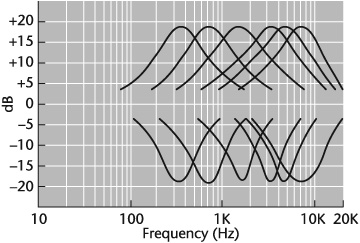
Figure 11-1. Bell curve or haystack showing 18 dB boost or cut at 350 Hz, 700 Hz, 1,600 Hz, 3,200 Hz, 4,800 Hz, and 7,200 Hz.
Shelving also increases or decreases amplitude by a fixed amount, gradually flattening out or shelving, at the maximum level when the chosen (called turnover or cutoff) frequency is reached. Level then remains constant at all frequencies beyond that point (see Figure 11-2).
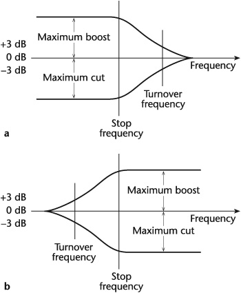
Figure 11-2. Low-frequency shelving equalization and (b) high-frequency shelving equalization. The turnover frequency shown is where the gain is 3 dB above (or below) the shelving level—in other words, the frequency where the equalizer begins to flatten out. The stop frequency is the point at which the gain stops increasing or decreasing.
In other words, with boost/cut EQ, when a frequency is selected for boost or cut by a certain amplitude, that frequency is the one most affected. Adjacent frequencies are also affected but by gradually lesser changes in level. With shelving EQ, all frequencies above (high-frequency shelving) or below (low-frequency shelving) the selected frequency are equally increased or decreased by the level selected.
The number of frequencies on equalizers varies. Generally, the frequencies are in full-, half-, and third-octave intervals. If the lowest frequency on a full-octave equalizer is, say, 50 Hz, the other frequencies ascend in octaves: 100 Hz, 200 Hz, 400 Hz, 800 Hz, and so on, usually to 12,800 Hz. A half-octave equalizer ascends in half octaves. If the lowest frequency is 50 Hz, the intervals are at or near 75 Hz, 100 Hz, 150 Hz, 200 Hz, 300 Hz, 400 Hz, 600 Hz, and so on. A third-octave equalizer would have intervals at or near 50 Hz, 60 Hz, 80 Hz, 100 Hz, 120 Hz, 160 Hz, 200 Hz, 240 Hz, 320 Hz, 400 Hz, 480 Hz, 640 Hz, and so on. Obviously, the more settings, the better the sound control—but at some cost. The more settings there are on an equalizer (or any device, for that matter), the more difficult it is to use correctly because problems such as added noise and phasing may be introduced, to say nothing of having to keep track of more control settings.
Two types of equalizers are in general use: fixed-frequency and parametric.
The fixed-frequency equalizer is so called because it operates at fixed frequencies usually selected from two (high and low), three (high, middle, and low), or four (high, upper-middle, lower-middle, and low) ranges of the frequency spectrum (see Figures 8-1 and 8-5). Typically, the high and low fixed-frequency equalizers on consoles are shelving equalizers. The midrange EQs are center-frequency boost/cut equalizers. Each group of frequencies is located at a separate control, but only one center frequency at a time per control may be selected. At or near each frequency selector is a level control that boosts or cuts the selected center and band frequencies. A fixed-frequency equalizer has a preset bandwidth—a range of frequencies on either side of the center frequency selected for equalizing that is also affected. The degrees of amplitude to which these frequencies are modified form the bandwidth curve. If you boost, say, 350 Hz a total of 18 dB, the bandwidth of frequencies also affected may go to as low as 80 Hz on one side and up to 2,000 Hz on the other. The peak of the curve is 350 Hz—the frequency that is boosted the full 18 dB. The adjacent frequencies are also boosted but to a lesser extent, depending on the bandwidth. Because each fixed-frequency equalizer can have a different fixed bandwidth and bandwidth curve, it is a good idea to study the manufacturer’s specifications before you use one. A measure of the bandwidth of frequencies an equalizer affects is known as the Q.
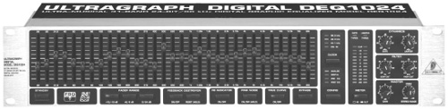
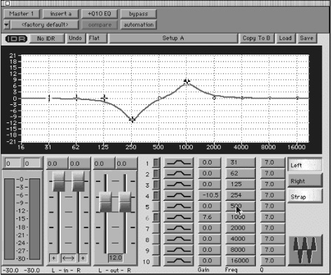
The graphic equalizer is a type of fixed-frequency equalizer. It consists of sliding, instead of rotating, controls that boost or attenuate selected frequencies. It is called “graphic” because the positioning of these controls gives a graphic representation of the frequency curve set. (The display does not include the bandwidth of each frequency, however.) Because each frequency on a graphic equalizer has a separate sliding control, it is possible to use as many as you wish simultaneously (see Figure 11-3).
The main difference between a parametric equalizer (see Figure 11-4) and a fixed-frequency equalizer is that the parametric has continuously variable frequencies and bandwidths, making it possible to change a bandwidth curve by making it wider or narrower, thereby altering the affected frequencies and their levels. This provides greater flexibility and more precision in controlling equalization. In other words, in parametric EQ, it is possible to vary the Q from anywhere between high-Q settings, which produce narrow bands of frequencies, to low-Q settings, which affect wider bands of frequencies (see Figure 11-5).
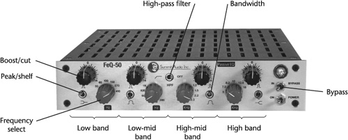
Figure 11-4. Parametric equalizer. This model includes four EQ bands, each with six switch-selectable frequencies and 14 dB of fully sweepable level increase or attenuation. The low-middle and high-middle are the parametric bands and can switch between narrow and wide bandwidths. The low- and high-frequency bands can switch between boost/cut and shelving EQ. Also included is a switchable high-pass filter at 30 Hz to reduce rumble.

A paragraphic equalizer combines the sliding controls of a graphic equalizer with the flexibility of parametric equalization (see Figure 11-6).
A filter is a device that attenuates certain bands of frequencies. It is a component of an equalizer. There are differences between attenuating with an equalizer and with a filter, however. First, with an equalizer, attenuation affects only the selected frequency and the frequencies on either side of it, whereas with a filter all frequencies above or below the selected frequency are affected. Second, an equalizer allows you to vary the amount of drop in loudness; with a filter, the drop is usually preset and relatively steep.
Among the most common filters are high-pass, low-pass, band-pass, and notch.
A high-pass (low-cut) filter attenuates all frequencies below a preset point; a low-pass (high-cut) filter attenuates all frequencies above a preset point (see Figure 11-7).
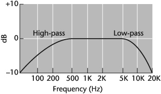
Suppose in a recording there is a bothersome rumble between 35 Hz and 50 Hz. By setting a high-pass filter at 50 Hz, all frequencies below that point are cut and the band of frequencies above it continues to pass—hence the name high-pass (low-cut) filter.
The low-pass (high-cut) filter works on the same principle but affects the higher frequencies. If there is hiss in a recording, you can get rid of it by setting a low-pass filter at, say, 10,000 Hz. This cuts the frequencies above that point and allows the band of frequencies below 10,000 Hz to pass through. But keep in mind that all sound above 10 kHz—the program material, if there is any, along with the hiss—will be filtered.
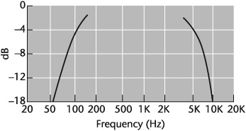
A band-pass filter is a device that sets high- and low-frequency cutoff points and permits the band of frequencies in between to pass (see Figure 11-8). Band-pass filters are used more for corrective rather than creative purposes.
A notch filter is also used mainly for corrective purposes. It can cut out an extremely narrow band, allowing the frequencies on either side of the notch to pass. For example, a constant problem in audio is AC (alternating current) hum, which has a frequency of 60 Hz. A notch filter can remove it without appreciably affecting the adjacent frequencies.
A psychoacoustic processor is designed to add clarity, definition, overall presence, and life, or “sizzle,” to program material. Some units add tone-generated odd and even harmonics[1] to the audio; others are fixed or program-adaptive, high-frequency equalizers. A psychoacoustic processor might also achieve its effect by adding comb filtering and by introducing narrow-band phase shifts between stereo channels. One well-known psychoacoustic processor is the Aphex Aural Exciter.
Time processors are devices that affect the time relationships of signals. These effects include reverberation and delay.
Reverberation, you will recall, is created by random, multiple, blended repetitions of a sound or signal. As these repetitions decrease in intensity, they increase in number. Reverberant sound increases average signal level and adds depth, spatial dimension, and additional excitement to the listening experience.
A reverberation effect has two main elements: the initial reflections and the decay of those reflections (see Chapter 1). Therefore, reverb results when the first reflections hit surfaces and continue to bounce around until they decay. In creating reverb electronically, using the parlance of audio, a signal is sent to the reverb processor as dry sound—without reverb—and is returned as wet sound—with reverb.
The types of reverb in current use are digital, convolution, plate, and acoustic chamber. Reverb plug-in software may be considered a fifth type. There is also spring reverberation, which is rarely employed today because of its mediocre sound quality. It is sometimes used, however, in guitar amplifiers because of its low cost, small size, and when the musician is going for the particular sound quality spring reverbs produce.
Digital reverberation is the most common today. Most digital reverb devices are capable of producing a variety of different acoustic environments. Generally, when fed into the circuitry and digitized, the signal is delayed for several milliseconds. The delayed signal is then recycled to produce the reverb effect. The process is repeated many times per second, with amplitude reduced to achieve decay.
Specifically, in digital reverb, numerous delay times create discrete echoes, followed by multiple repetitions of these initial delays to create the ambience, which continues with decreasing clarity and amplitude. High-quality digital reverb units are capable of an extremely wide range of effects, produce high-quality sound, and take up relatively little room.
Digital reverb systems can simulate a variety of acoustical and mechanical reverberant sounds such as small and large concert halls, bright- and dark-sounding halls, small and large rooms, and small and large reverb plates (see “Plate Reverberation” later in this chapter). With each effect, it is also possible to control individually the attack; decay; diffusion (density); high-, middle-, and low-frequency decay times; and other sonic colorings.
One important feature of most digital reverb units is predelay—the amount of time between the onset of the direct sound and the appearance of the first reflections. Predelay is essential for creating a believable room ambience because early reflections arrive before reverberation. It also helps create the perception of a room’s size: Shorter predelay times give the sense of a smaller room and vice versa.
Most digital reverb systems are programmed and programmable. They come with preprogrammed effects but also permit new ones to be programmed in and stored for reuse (see Figure 11-9).
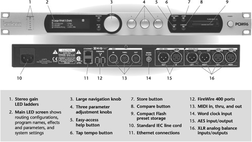
Figure 11-9. Digital reverberation processor, front and rear views. This model includes monaural and stereo reverbs for 28 effects, including chamber, hall, plate, room, chorus/flange, and delay. There are digital audio workstation automation and FireWire streaming through a plug-in format, compact Flash preset storage, and sampling rates of 44.1 kHz, 48 kHz, 88.2 kHz, and 96 kHz.
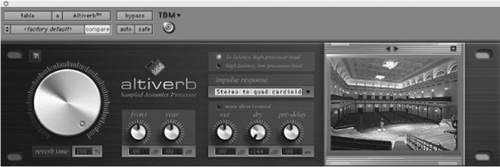
Convolution reverb is a sample-based process that multiplies the spectrums of two audio files. One file represents the acoustic signature of an acoustic space. It is called the impulse response (IR). The other file is the source, or carrier. It takes on the characteristics of the acoustic space when it is multiplied by the IR. Hence, it has the quality of having been recorded in that space. By facilitating the interaction of any two arbitrary audio files, convolution reverb provides a virtually infinite range of unusual sonic possibilities.
Among the more common uses of convolution reverb is providing the actual likeness of real acoustic spaces interacting with any sound source you wish such as Boston’s Symphony Hall, Nashville’s Ryman Auditorium, a particular recording stage, a living room, a kitchen, or a jail cell (see Figure 11-10). The process can create effects such as exotic echoes and delays, a single clave or marimba hit, and different tempos and timbres.
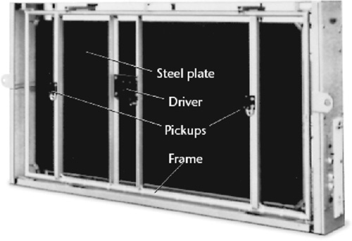
The reverberation plate is a mechanical-electronic device consisting of a thin steel plate suspended under tension in an enclosed frame (see Figure 11-11). It is large and heavy and requires isolation in a separate room. A moving-coil driver, acting like a small speaker, vibrates the plate, thus transducing the electrical signals from the console into mechanical energy. A contact microphone (two for stereo) picks up the plate’s vibrations, transduces them back into electric energy, and returns them to the console. The multiple reflections from the vibrating plate create the reverb effect.
The acoustic reverberation chamber is a natural and realistic type of simulated reverb because it works on acoustic sound in an acoustic environment. It is a room with sound-reflective surfaces and nonparallel walls to avoid flutter echoes—multiple echoes at a rapid, even rate—and standing waves—apparently stationary waveforms created by multiple reflections between opposite, usually parallel, room surfaces. It usually contains two directional microphones (for stereo), placed off room center, and a loudspeaker, usually near a corner angled or back-to-back to the mic(s) to minimize the amount of direct sound the mic(s) pick up. The dry sound feeds from the console through the loudspeaker, reflects around the chamber, is picked up by the mic(s), and is fed back wet into the console for further processing and routing.
In considering a reverberation system, it is helpful to keep in mind that reverberation and ambience, often thought of as synonymous, are different. Reverb is the remainder of sound that exists in a room after the source of the sound is stopped.[2] Ambience refers to the acoustical qualities of a listening space, including reverberation, echoes, background noise, and so on.[3] In general, reverb adds spaciousness to sound; ambience adds solidity and body.
Delay is the time interval between a sound or signal and its repetition. By manipulating delay times, it is possible to create a number of echo effects (see “Uses of Delay” later in this chapter). This is done most commonly with an electronic digital delay.
Digital delay is generated by routing audio through an electronic buffer. The information is held for a specific period of time, which is set by the user, before it is sent to the output. A single-repeat delay processes the sound only once; multiple delays process the signal over and over. The amount and the number of delay times vary with the unit (see Figure 11-12).
Two parameters about delay that are important to understand are delay time and feedback. Delay time regulates how long a given sound is held and therefore the amount of time between delays. Feedback, also known as regeneration, controls how much of that delayed signal is returned to the input. Raising the amount of feedback increases the number of repeats and the length of decay. Turning it down completely generates only one repeat.
The better digital delays have excellent signal-to-noise ratio, low distortion, good high-frequency response with longer delay times, and an extensive array of effects. They are also excellent for prereverb delay. Lower-grade units are not as clean-sounding, and high-frequency response is noisier with longer delay times.
Delay has a number of creative applications. Among the common effects are doubling, chorus, slap back echo, and prereverb delay.
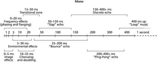
Doubling—. One popular use of delay is to fatten sound. The effect, which gives an instrument or voice a fuller, stronger sound, is called doubling. It is created by setting the delay to about 15 to 35 ms. These short delays are like early sound reflections and lend a sense of openness or ambience to dead-sounding instruments or voices.
Doubling can also be done live by recording one track and then overdubbing the same part on a separate track in synchronization with the first. Because it is not possible to repeat a performance exactly, variations in pitch, timing, and room sounds add fullness or openness to sound. By continuing this process, it is possible to create a chorus effect.
Chorus—. The chorus effect is achieved by recirculating the doubling effect. The delay time is about the same as in doubling—15 to 35 ms—but is repeated. This effect can make a single voice sound like many and add spaciousness to a sound. Two voices singing in a relatively dead studio can be made to sound like a choir singing in a hall by chorusing the original sound.
Slap back echo—. A slap back echo is a delayed sound perceived as a distinct echo, much like the discrete Ping-Pong sound emitted by sonar devices when a contact is made. Slap back delay times are generally short, about 50 to 150 ms.
Prereverb delay—. As mentioned in the discussion of digital reverb, there is a definite time lag between the arrival of direct waves from a sound source and the arrival of reflected sound in acoustic conditions. In some reverb systems, there is no delay between the dry and wet signals. By using a delay unit to delay the input signal before it gets to the reverb unit, it is possible to improve the quality of reverberation, making it sound more natural.
Flanging is produced electronically. The signal is combined with its time-delayed replica. Delay time is relatively short, from 0 to 20 ms. Ordinarily, the ear cannot perceive time differences between direct and delayed sounds that are this short. But due to phase cancellations when the direct and delayed signals are combined, the result is a comb-filter effect—a series of peaks and dips in the frequency response. This creates a filtered tone quality that sounds hollow, swishy, and outer space-like.
In addition to the various delay times, flangers typically provide feedback rate and depth controls. Feedback rate determines how quickly a delay time is modulated; for example, a feedback rate setting of 0.1 Hz performs one cycle sweep every 10 seconds. Depth controls adjust the spread between minimum and maximum delay times; depth is expressed as a ratio.
Many flangers provide controls to delay feedback in phase or out of phase. In-phase flanging is “positive”—the direct and delayed signals have the same polarity. Positive flanging accents even harmonics, producing a metallic sound. Out-of-phase flanging is “negative”—the two signals are opposite in polarity and accents odd harmonics. Negative flanging can create strong, sucking effects like a sound turned inside out.
Phasing and flanging are similar in the way they are created. In fact, it is sometimes difficult to differentiate between the two. Instead of using a time-delay circuit, however, phasers use a phase shifter. Delays are very short, between 0 ms and 10 ms. The peaks and dips are more irregular and farther apart than in flanging, which results in something like a wavering vibrato that pulsates or undulates. Phasers provide a less pronounced pitched effect than flangers because their delay times are slightly shorter and the phasing effect has less depth than with flanging.
Phasers use two parameters that control modulation of the filters: rate (or speed) and depth (or intensity). Rate determines the sweep speed between the minimum and the maximum values of the frequency range. Depth defines the width of that range between the lowest and the highest frequencies.
Morphing is the continuous, seamless transformation of one effect (aural or visual) into another. It is more than a sophisticated dissolve (the sonic counterpart of a dissolve is the crossfade). Morphing is a complete restructuring of two completely different and independent effects. Because most audio-morphing effects are delay-based, audio-morphing devices can be classified as time processors (see Figure 11-13).
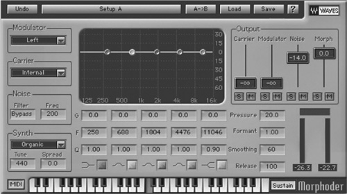
Figure 11-13. Morphing. This plug-in, called the Morphoder, is a processor of the vocoder type (see “Voice Processors” later in this chapter). It allows two audio signals to be combined using one source as a modulator input and a synthesizer as the carrier. The effect is that the synthesizer will “talk” and actually say the words spoken by the voice; or a drum track can be the modulator, resulting in a rhythmic keyboard track in sync with the drum track.
A few examples of audio morphing include turning human speech or vocal lines into lines impossible to be spoken or sung by a human; turning sounds that exist into sounds that do not exist; spinning vowel-like sounds, varying their rate and depth, and then freezing them until they fade away; flanging cascades of sound across stereo space, adding echo, and varying the envelope control of rates; adding echoing rhythms to a multivoice chorus that become more dense as they repeat, with the effect growing stronger as the notes fade away; and taking a musical instrument and adding pitch sweeps that dive into a pool of swirling echoes that bounce from side to side or end by being sucked up.
Amplitude, or dynamic, processors are devices that affect dynamic range. These effects include such functions as compression, limiting, de-essing, expanding, noise gating, and pitch shifting.
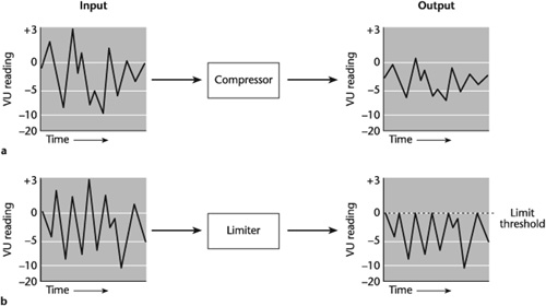
The term compressor is customarily linked with the term limiter. They do basically the same signal processing but to different degrees. The compressor is a processor whose output level increases at a slower rate as its input level increases (see Figure 11-14). It is used to restrict dynamic range because of the peak signal limitations of an electronic system, for artistic goals, due to the surrounding acoustical requirements, or any combination of these factors.
Compressors usually have four basic controls—for compression ratio, compression threshold, attack time, and release time—each of which can affect the others. Some compressors also include a makeup gain control. Compressor plug-ins may have additional features that act on a signal’s dynamics.
The compression ratio establishes the proportion of change between the input and the output levels. The ratios are usually variable and, depending on the compressor, there are several selectable points between 1.1:1 and 20:1. Some recent compressor designs change ratios instantaneously, depending on the program’s dynamic content and the range of control settings. If you set the compression ratio for, say, 2:1, it means that for every 2 dB increase of the input signal, the output will increase by 1 dB; at 5:1, a 5 dB increase of the input signal increases the output by 1 dB. In other words, it “reins in” excessive program dynamics. This is how sound with a dynamic range greater than what the equipment can handle is brought to usable proportions before distortion occurs.
The compression threshold is the level at which compression ratio takes effect. It is an adjustable setting and is usually selected based on a subjective judgment of where compression should begin. It is difficult to predetermine what settings will work best for a given sound at a certain level; it is a matter of listening and experimenting. The compressor has no effect on the signal below the threshold-level setting. For an illustration of the relationship between compression ratio and threshold, see Figure 11-15.
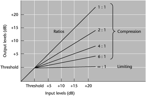
Figure 11-15. The relationship of various compression ratios to a fixed threshold point. The graph also displays the difference between the effects of limiting and compression.
Once the threshold is reached, compression begins, reducing the gain according to the amount the signal exceeds the threshold level and according to the ratio set. The moment the compressor starts gain reduction is called the knee. Hard knee compression is abrupt; soft knee compression is smoother and less apparent.
Attack time is the length of time it takes the compressor to start compressing after the threshold has been reached. In a good compressor, attack times range from 500 microseconds (μs) to 100 ms. Depending on the setting, an attack time can enhance or detract from a sound. If the attack time is long, it can help bring out percussive attacks; but if it is too long, it can miss or overshoot the beginning of the compressed sound. If the attack time is too short, it reduces punch by attenuating the attacks, sometimes producing popping or clicking sounds. When it is controlled, a short attack time can heighten transients and add a crisp accent to sound. Generally, attack time should be set so that signals exceed the threshold level long enough to cause an increase in the average level. Otherwise, gain reduction will decrease overall level. Again, your ear is the best judge of the appropriate attack time setting.
Release time, or recovery time, is the time it takes a compressed signal to return to normal (unity gain) after the input signal has fallen below the threshold. Typical release times vary from 20 ms to several seconds. It is perhaps the most critical variable in compression because it controls the moment-to-moment changes in the level and therefore the overall loudness. One purpose of the release-time function is to make imperceptible the variations in loudness level caused by the compression. For example, longer release times are usually applied to music that is slower and more legato (that is, smoother and more tightly connected); shorter release times are usually applied to fast music.
Generally, release times should be set long enough that if signal levels repeatedly rise above the threshold, they cause gain reduction only once. If the release time is too long, a loud section of the audio could cause gain reduction that continues through a soft section.
These suggestions are not to imply rules—they are only guidelines. In fact, various release times produce different effects. Some enhance sound, others degrade it. See Chapter 13 for a list of the different effects compression produces and several of the applications that compressors (and limiters) have.
One additional important compressor control is called makeup gain. It allows adjustment of the output level to the desired optimum. It is used, for example, when loud parts of a signal are so reduced that the overall result sounds too quiet.
Compressors fall into two categories: broadband and split-band. A broadband compressor acts on the dynamic range of the input signal across the entire frequency spectrum. The split-band compressor affects an input signal independently by splitting the audio into multiple bands, as needed, and then recombining the outputs of the bands into a single mono or stereo broadband signal. Good split-band compressors provide separate threshold, ratio control, attack and release times, and makeup gain for each compression band (see Figure 11-16).
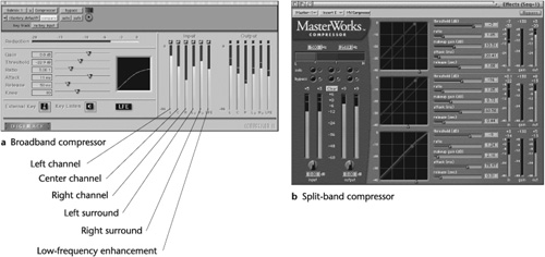
Figure 11-16. Compressor plug-ins. (a) A broadband compressor that can be used to control the dynamic range in recording and mixing 5.1 surround sound. (b) A split-band compressor that provides three separate bands of compression with graphic, adjustable crossover points among the three. Each band has its own settings, facilitating control over the entire spectrum of the signal being compressed, and a solo control that isolates an individual band for separate monitoring. This model has 64-bit processing and metering with numerical peak and RMS (root mean square) value displays.
The split-band compressor allows for finer control of dynamic range. For example, a bass can be compressed in the low end without adversely affecting the higher end. Conversely, speech can be de-essed without losing fullness in the lower end.
The limiter is a compressor whose output level stays at or below a preset point regardless of the input level. It has a compression ratio between 10:1 and infinity; it puts a ceiling on the loudness of a sound at a preset level (see Figure 11-14). Regardless of how loud the input signal is, the output will not go above this ceiling. This makes the limiter useful in situations where high sound levels are frequent or where a performer or console operator cannot prevent loud sounds from going into the red.
The limiter has a preset compression ratio but a variable threshold; the threshold sets the point where limiting begins. Attack and release times, if not preset, should be relatively short, especially the attack time. A short attack time is usually essential to a clean-sounding limit.
Unlike compression, which can have little effect on the frequency response, limiting can reduce high-frequency response. Also, if limiting is severe, the signal-to-noise ratio drops dramatically. What makes a good limiter? One that is used infrequently but effectively, that is, except in broadcasting, where limiting the signal before transmission is essential to control peak levels and hence overload distortion.
The de-esser is basically a fast-acting compressor that acts on high frequencies by attenuating them. It gets rid of the annoying hissy consonant sounds such as s, z, ch, and sh in speech and vocals. A de-esser may be a stand-alone unit or, more common, built into compressors and voice processors.
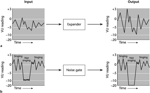
An expander, like a compressor, affects dynamic range (see Figure 11-17a). But whereas a compressor reduces it, an expander increases it. Like a compressor, an expander has variable ratios and is triggered when sound reaches a set threshold level. The ratios on an expander, however, are the inverse of those on a compressor but are usually gentler: 1:2, 1.5:2, and so on. At 1:2, each 1 dB of input expands to 2 dB of output; at 1:3, each 1 dB of input expands to 3 dB of output. Because an expander is triggered when a signal falls below a set threshold, it is commonly used as a noise gate.
Like the compressor, the expander/noise gate has the same dynamic determinants but they act inversely to those of the compressor. In addition to ratio settings, there is threshold: When the input signal level drops below the threshold, the gate closes and mutes the output. When the input signal level exceeds the threshold, the gate opens. Attack time determines how long it takes for the gate to go from full off to full on once the input level exceeds the threshold. Attack times are usually quite short—1 ms or even less. Longer attacks tend to chop off fast transients on percussive sounds. Release time sets the time required for the gate to go from full on to full off once the signal level falls below the threshold. Another control is the key input, sometimes called a side chain input, which allows a different signal to be fed in to govern the gating action such as using a bass drum as the key signal to turn another sound on and off in time with the bass drum’s rhythm.
The noise gate is used primarily as a fix-it tool to reduce or eliminate unwanted low-level noise from amplifiers, ambience, rumble, noisy tracks, and leakage. It also has creative uses, however, to produce dynamic special effects. As an example of a practical application, assume you have two microphones—one for a singer and one for an accompanying piano. When the singer and the pianist are performing, the sound level will probably be loud enough to mask unwanted low-level noises. But if the pianist is playing quietly and the vocalist is not singing, or vice versa, the open, unused microphone may pick up these noises (see Figure 11-17b).
An obvious solution to this problem is to turn down the fader when a microphone is not being used, cutting it off acoustically and electronically; but this could become hectic for a console operator if several sound sources need to be coordinated. Another solution is to set the expander’s threshold level at a point just above the quietest sound level that the vocalist (or piano) emits. When the vocalist stops singing, the loudness of the sound entering the mic falls below the threshold point of the expander, which shuts down, or gates, the mic. When a signal is above the threshold, there is no gating action and therefore no removal of noise.
The key to successful noise gating is in the coordination of the threshold and the ratio settings. Because there is often little difference between the low level of a sound’s decay and the low level of noise, in gating noise you have to be wary that you do not cut off program material as well. Always be careful when you use a noise gate; unless it is set precisely, it can adversely affect response.
A pitch shifter is a device that uses both compression and expansion to change the pitch of a signal. It is used to correct minor off-pitch problems, create special effects, or change the length of a program without changing its pitch. The latter function is called time compression/expansion. For example, if a singer delivers a note slightly flat or sharp, it is possible to raise or lower the pitch so that it is in tune. A pitch shifter also allows an input signal to be harmonized by mixing it with the harmonized signal at selected pitch ratios.
A pitch shifter works by compressing and expanding audio data. When the audio is compressed, it runs faster and raises pitch; it also shortens the audio segment. When the audio is expanded, it lowers pitch and lengthens the audio data. During processing, therefore, the pitch shifter is also rapidly cutting and pasting segments of data at varying intervals.
The basic parameter for pitch shifting is transposition. Transposing is changing the original pitch of a sound into another pitch; in music, it is changing into another key. Transposition sets the harmony-line interval, typically within a range of one or two octaves. A pitch shifter may also include a delay line with feedback and predelay controls.
Depending on the model or software, a pitch shifter may also be capable of speed-up pitch-shifting, which changes the timbre and pitch of natural sounds. Speed-up pitch-shifting is sometimes referred to as the “chipmunk effect.”
As a time compressor, a pitch shifter can shorten recorded audio material with no editing, no deletion of content, and no alteration in pitch (see Figure 11-18).
Noise processors reduce or eliminate noise from an audio signal. With the advent of digital signal processing (DSP) plug-ins, these processors have become powerful tools in getting rid of virtually any unwanted noise. In fact, because noise reduction with digital processing is so effective, getting rid of recorded and system noise has become far less of a problem than it once was. It has also been a boon to audio restoration.
Software programs are dedicated to getting rid of different types of noise such as clicks, crackles, pops, hum, buzz, rumble, computer-generated noise, unwanted background ambience, and recovery of lost signals due, for example, to clipping. They are available in bundles with separate programs for particular types of noise reduction.
Digital noise reduction is able to remove constant, steady noises. In a vocal track with high-level background noise from lights, ventilating fans, and studio acoustics, almost all of the noise can be removed without affecting voice quality.
In digital noise reduction, there are parameters to control and balance. It is important to consider the amount of noise removed from the signal, the amount of signal removed from the program material, and the amount of new sonic colorations added to the signal. Failure to coordinate these factors can sonically detract from the program material if not exacerbate the original noise problem.
The following are other points to consider when using noise reduction [4]
Always preview before processing and have a backup copy.
To maintain perspective, continue to compare the processed sound against the unprocessed sound.
Do not rely only on automatic settings. They may not precisely produce the desired effect or may introduce unwanted artifacts, or both.
Use the “noise only” monitoring feature to check the part of the audio removed by the software.
In heavy noise situations, a multiband expander or an EQ boost in the frequency range of the target audio helps make the audio clearer.
In rhythmic material, be careful that the noise reduction processing does not adversely affect the rhythmic patterns or the transient response.
A multieffects signal processor combines several of the functions of individual signal processing in a single unit. The variety and the parameters of these functions vary with the unit; but because most multieffects processors are digital, they are powerful audioprocessing tools albeit, in some cases, dauntingly complicated. Multieffects processors are available in stand-alone units, plug-ins, and plug-in bundles, and most have wide frequency response, at least 16-bit resolution, and dozens of programmable presets.
One type of popular multieffects processor used for voice work is the voice processor (also referred to as a vocoder). Because of its particular application in shaping the sound of the all-important spoken and singing voice, it warrants some attention here.
A voice, or vocal, processor can enhance, modify, pitch-correct, harmonize, and change completely the sound of a voice, even to the extent of gender. Functions vary with the model, but in general a system may include some, many, or most of the following: preamp, EQ, harmonizer, compression, noise gate, reverb, delay, and chorus.
Voice-modeling menus create different textures and may include any number of effects for inflections; spectral changes in frequency balance; vibratos (variations in the frequency of a sound generally at a rate of 2 and 15 times per second; glottals (breathiness, rasp, and growl); warp (changes in formants—a frequency band in a voice or musical instrument that contains more energy and loudness than the neighboring area); harmony processing that provides multivoice harmonies; and pitch shifting in semitones, or in cents—1/100 semitone. Voice processors are available in rack-mounted models and as plug-ins.
In addition to plug-ins that perform the relatively familiar signal-processing functions, specialized plug-ins add an almost infinite amount of flexibility to sound shaping. Among the hundreds available are programs for mastering—the final stage in preparing audio material for duplication; stereo and surround-sound calibration, panning, and mixing; musical synthesis with patches included; virtual instrumentation of just about any musical sound source such as keyboards, fretted instruments, horns, drums, and full orchestras; metering, metronome, and instrument tuning; time alignment of vocals, dialogue, and musical instruments; simulation of various types of guitar amplifiers; software sampling with multiformat sound libraries; and emulation—making digital audio sound like analog.
Plug-ins come in a number of different formats. Before purchasing one, make sure it is compatible with your software production system. For example, the most popular formats for Windows are Steinberg’s Virtual Studio Technology (VST) and Direct X, a group of application program interfaces. Because formats come and go, as do software programs, listing here which plug-in formats are compatible with which production systems would be unwieldy and become quickly outdated. A check of vendors’ websites can provide their available plug-ins and the systems with which they are compatible.
Signal processors are used to alter some characteristic of a sound. They can be grouped into four categories: spectrum; time; amplitude, or dynamic; and noise.
Signal processors may be inboard, incorporated into production consoles; outboard stand-alone units; or a plugin—an add-on software tool that gives a digital recording/editing system signal-processing alternatives beyond what the original system provides.
The equalizer and the filter are examples of spectrum processors because they alter the spectral balance of a signal. The equalizer increases or decreases the level of a signal at a selected frequency by boost or cut (also known as peak and dip) or by shelving. The filter attenuates certain frequencies above, below, between, or at a preset point(s).
Common types of equalizers in use are the fixed-frequency, parametric, graphic, and paragraphic.
The most common filters are high-pass (low-cut), low-pass (high-cut), band-pass, and notch.
Psychoacoustic processors add clarity, definition, and overall presence to sound.
Time processors affect the time relationships of signals. Reverberation and delay are two such effects.
The four types of reverberation systems used for the most part today are digital, convolution, plate, and acoustic chamber; reverb plug-in software may be considered a fifth type.
Digital reverb reproduces electronically the sound of different acoustic environments.
Convolution reverb is a sample-based process that multiplies the spectrums of two audio files. One file represents the acoustic signature of an acoustic space. It is called the impulse response (IR). The other file, or source, takes on the characteristics of the acoustic space when it is multiplied by the IR. Hence, it has the quality of having been recorded in that space.
The reverberation plate is a mechanical-electronic device consisting of a thin steel plate suspended under tension in an enclosed frame, a moving-coil driver, and a contact microphone(s).
The acoustic reverberation chamber is a natural and realistic type of simulated reverb because it works on acoustic sound in an acoustic environment with sound-reflective surfaces.
An important feature of most digital reverb units is predelay—the amount of time between the onset of the direct sound and the appearance of the first reflections.
Delay is the time interval between a sound or signal and its repetition.
Delay effects, such as doubling, chorus, slap back echo, and prereverb delay, are usually produced electronically with a digital delay device.
Flanging and phasing split a signal and slightly delay one part to create controlled phase cancellations that generate a pulsating sound. Flanging uses a time delay; phasing uses a phase shifter.
Morphing is the continuous, seamless transformation of one effect (aural or visual) into another.
Amplitude (dynamic) processors affect a sound’s dynamic range. These effects include compression, limiting, de-essing, expanding, noise gating, and pitch shifting.
With compression, as the input level increases, the output level also increases but at a slower rate, reducing dynamic range. With limiting, the output level stays at or below a preset point regardless of its input level. With expansion, as the input level increases, the output level also increases but at a greater rate, increasing dynamic range.
A broadband compressor acts on the dynamic range of the input signal across the entire frequency spectrum. The split-band compressor affects an input signal independently by splitting the audio into multiple bands, as needed, and then recombining the outputs of the bands into a single mono or stereo broadband signal.
A de-esser is basically a fast-acting compressor that acts on high-frequency sibilance by attenuating it.
An expander, like a compressor, affects dynamic range. But whereas a compressor reduces it, an expander increases it.
A noise gate is used primarily to reduce or eliminate unwanted low-level noise such as ambience and leakage. It is also used creatively to produce dynamic special effects.
A pitch shifter uses both compression and expansion to change the pitch of a signal or the running time of a program.
Noise processors are designed to reduce or eliminate such noises as clicks, crackles, hum, and rumble from an audio signal.
Multieffects signal processors combine several of the functions of individual signal processorsin a single unit.
A voice, or vocal, processor (also referred to as a vocoder) can enhance, modify, pitch-correct, harmonize, and change completely the sound of a voice, even to the extent of gender.
Highly specialized plug-ins add an almost infinite amount of flexibility to sound shaping.
When selecting a plug-in, it is important to know whether it is compatible with the software production system used.
[1] Each harmonic or set of harmonics adds a characteristic tonal color to sound, although they have less effect on changes in timbre as they rise in pitch above the fundamental. In general, even-numbered harmonics—second, fourth, and sixth—create an open, warm, filled-out sound. The first two even harmonics are one and two octaves above the fundamental, so the tones blend. Odd-numbered harmonics—third and fifth—produce a closed, harsh, stopped-down sound. The first two odd harmonics are an octave plus a fifth and two octaves plus a major third above the fundamental, which bring their own tonality to the music.
[2] Glenn D. White and Gary J. Louie, The Audio Dictionary, 3rd ed. (Seattle: University of Washington Press, 2005), p. 331.
[3] Ibid, p. 16.
[4] Based on Mike Levine, “Noises Off,” Electronic Musician, August, 2008, p. 50.