
Chapter 5. Ecommerce
In this chapter, we’ll look at how MongoDB fits into the world of retail, particularly in two main areas: maintaining product catalog data and inventory management. Our first use case, Product Catalog, deals with the storage of product catalog data.
Our next use case, Category Hierarchy, examines the problem of maintaining a category hierarchy of product items in MongoDB.
The final use case in this chapter, Inventory Management, explores the use of MongoDB in an area a bit outside its traditional domain: managing inventory and checkout in an ecommerce system.
Product Catalog
In order to manage an ecommerce system, the first thing you need is a product catalog. Product catalogs must have the capacity to store many different types of objects with different sets of attributes. These kinds of data collections work quite well with MongoDB’s flexible data model, making MongoDB a natural fit for this type of data.
Solution Overview
Before delving into the MongoDB solution, we’ll examine the ways in which relational data models address the problem of storing products of various types. There have actually been several different approaches that address this problem, each with a different performance profile. This section examines some of the relational approaches and then describes the preferred MongoDB solution.
Concrete-table inheritance
One approach in a relational model is to create a table for each product category. Consider the following example SQL statement for creating database tables:
CREATETABLE`product_audio_album`(`sku`char(8)NOTNULL,...`artist`varchar(255)DEFAULTNULL,`genre_0`varchar(255)DEFAULTNULL,`genre_1`varchar(255)DEFAULTNULL,...,PRIMARYKEY(`sku`))...CREATETABLE`product_film`(`sku`char(8)NOTNULL,...`title`varchar(255)DEFAULTNULL,`rating`char(8)DEFAULTNULL,...,PRIMARYKEY(`sku`))...
This approach has limited flexibility for two key reasons:
- You must create a new table for every new category of products.
- You must explicitly tailor all queries for the exact type of product.
Single-table inheritance
Another relational data model uses a single table for all product categories and adds new columns any time you need to store data regarding a new type of product. Consider the following SQL statement:
CREATETABLE`product`(`sku`char(8)NOTNULL,...`artist`varchar(255)DEFAULTNULL,`genre_0`varchar(255)DEFAULTNULL,`genre_1`varchar(255)DEFAULTNULL,...`title`varchar(255)DEFAULTNULL,`rating`char(8)DEFAULTNULL,...,PRIMARYKEY(`sku`))
This approach is more flexible than concrete-table inheritance: it
allows single queries to span different product types, but at the
expense of space. It also continues to suffer from a lack of flexibility in
that adding new types of product requires a potentially expensive ALTER TABLE operation.
Multiple-table inheritance
Another approach that’s been used in relational modeling is multiple-table inheritance where you represent common attributes in a generic “product” table, with some variations in individual category product tables. Consider the following SQL statement:
CREATETABLE`product`(`sku`char(8)NOTNULL,`title`varchar(255)DEFAULTNULL,`description`varchar(255)DEFAULTNULL,`price`,...PRIMARYKEY(`sku`))CREATETABLE`product_audio_album`(`sku`char(8)NOTNULL,...`artist`varchar(255)DEFAULTNULL,`genre_0`varchar(255)DEFAULTNULL,`genre_1`varchar(255)DEFAULTNULL,...,PRIMARYKEY(`sku`),FOREIGNKEY(`sku`)REFERENCES`product`(`sku`))...CREATETABLE`product_film`(`sku`char(8)NOTNULL,...`title`varchar(255)DEFAULTNULL,`rating`char(8)DEFAULTNULL,...,PRIMARYKEY(`sku`),FOREIGNKEY(`sku`)REFERENCES`product`(`sku`))...
Multiple-table inheritance is more space-efficient than single-table inheritance
and somewhat more flexible than concrete-table inheritance. However, this model does
require an expensive JOIN operation to obtain all attributes
relevant to a product.
Entity attribute values
The final substantive pattern from relational modeling is the
entity-attribute-value (EAV) schema, where you would create a meta-model for
product data. In this approach, you maintain a table with three columns (e.g., entity_id, attribute_id, and value), and these triples describe
each product.
Consider the description of an audio recording. You may have a series of rows representing the following relationships:
Entity | Attribute | Value |
sku_00e8da9b | type | Audio Album |
sku_00e8da9b | title | A Love Supreme |
sku_00e8da9b | … | … |
sku_00e8da9b | artist | John Coltrane |
sku_00e8da9b | genre | Jazz |
sku_00e8da9b | genre | General |
… | … | … |
This schema is completely flexible:
- Any entity can have any set of any attributes.
- New product categories do not require any changes to the data model in the database.
There are, however, some significant problems with the EAV schema. One major
issue is that all nontrivial queries require large numbers of JOIN
operations. Consider retrieving the title, artist, and two genres for each item
in the table:
SELECTentity,t0.valueAStitle,t1.valueASartist,t2.valueASgenre0,t3.valueasgenre1FROMeavASt0LEFTJOINeavASt1ONt0.entity=t1.entityLEFTJOINeavASt2ONt0.entity=t2.entityLEFTJOINeavASt3ONt0.entity=t3.entity;
And that’s only bringing back four attributes! Another problem illustrated by this example is that the queries quickly become difficult to create and maintain.
Avoid modeling product data altogether
In addition to all the approaches just outlined, some ecommerce solutions with
relational database systems skip relational modeling altogether, choosing instead
to serialize all the product data into a BLOB column. Although the schema is
simple, this approach makes sorting and filtering on any data embedded in the
BLOB practically impossible.
The MongoDB answer
Because MongoDB is a nonrelational database, the data model for your product catalog can benefit from this additional flexibility. The best models use a single MongoDB collection to store all the product data, similar to the single-table inheritance model in Single-table inheritance.
Unlike single-table inheritance, however, MongoDB’s dynamic schema means that the individual documents need not conform to the same rigid schema. As a result, each document contains only the properties appropriate to the particular class of product it describes.
At the beginning of the document, a document-based schema should contain general
product information, to facilitate searches of the entire catalog. After the
common fields, we’ll add a details subdocument that contains fields that vary
between product types. Consider the following example document for an album product:
{sku:"00e8da9b",type:"Audio Album",title:"A Love Supreme",description:"by John Coltrane",asin:"B0000A118M",shipping:{weight:6,dimensions:{width:10,height:10,depth:1},},pricing:{list:1200,retail:1100,savings:100,pct_savings:8},details:{title:"A Love Supreme [Original Recording Reissued]",artist:"John Coltrane",genre:["Jazz","General"],...tracks:["A Love Supreme, Part I: Acknowledgement","A Love Supreme, Part II: Resolution","A Love Supreme, Part III: Pursuance","A Love Supreme, Part IV: Psalm"],},}
A movie item would have the same fields for general product information,
shipping, and pricing, but different fields for the details subdocument. Consider
the following:
{sku:"00e8da9d",type:"Film",...,asin:"B000P0J0AQ",shipping:{...},pricing:{...},details:{title:"The Matrix",director:["Andy Wachowski","Larry Wachowski"],writer:["Andy Wachowski","Larry Wachowski"],...,aspect_ratio:"1.66:1"},}
Operations
For most deployments, the primary use of the product catalog is to perform search operations. This section provides an overview of various types of queries that may be useful for supporting an ecommerce site. Our examples use the Python programming language, but of course you can implement this system using any language you choose.
Find products sorted by percentage discount descending
Most searches will be for a particular type of product (album, movie, etc.), but in some situations you may want to return all products in a certain price range or discount percentage.
For example, the following query returns all products with a discount greater than 25%, sorted by descending percentage discount:
query=db.products.find({'pricing.pct_savings':{'$gt':25})query=query.sort([('pricing.pct_savings',-1)])
To support this type of query, we’ll create an index on the pricing.pct_savings field:
db.products.ensure_index('pricing.pct_savings')
Note
Since MongoDB can read indexes in ascending or descending order, the order of the index does not matter when creating single-element indexes.
Find albums by genre and sort by year produced
The following returns the documents for the albums of a specific genre, sorted in reverse chronological order:
query=db.products.find({'type':'Audio Album','details.genre':'jazz'})query=query.sort([('details.issue_date',-1)])
In order to support this query efficiently, we’ll create a compound index on the properties used in the filter and the sort:
db.products.ensure_index([('type',1),('details.genre',1),('details.issue_date',-1)])
Note
The final component of the index is the sort field. This allows MongoDB to traverse the index in the sorted order and avoid a slow in-memory sort.
Find movies based on starring actor
Another example of a detail field-based query would be one that selects films
that a particular actor starred in, sorted by issue date:
query=db.products.find({'type':'Film','details.actor':'Keanu Reeves'})query=query.sort([('details.issue_date',-1)])
To support this query, we’ll create an index on the fields used in the query:
db.products.ensure_index([('type',1),('details.actor',1),('details.issue_date',-1)])
This index begins with the type field and then narrows by the other
search field, where the final component of the index is the sort field
to maximize index efficiency.
Find movies with a particular word in the title
In most relational and document-based databases, querying for a single word within a string-type field requires scanning, making this query much less efficient than the others mentioned here.
One of the most-requested features of MongoDB is the so-called full-text index, which makes queries such as this one more efficient. In a full-text index, the individual words (sometimes even subwords) that occur in a field are indexed separately. In exciting and recent (as of the writing of this section) news, development builds of MongoDB currently contain a basic full-text search index, slated for inclusion in the next major release of MongoDB. Until MongoDB full-text search index shows up in a stable version of MongoDB, however, the best approach is probably deploying a separate full-text search engine (such as Apache Solr or ElasticSearch) alongside MongoDB, if you’re going to be doing a lot of text-based queries.
Although there is currently no efficient full-text search support within MongoDB, there is
support for using regular expressions (regexes) with queries. In Python, we can pass a
compiled regex from the re module to the find() operation directly:
importrere_hacker=re.compile(r'.*hacker.*',re.IGNORECASE)query=db.products.find({'type':'Film','title':re_hacker})query=query.sort([('details.issue_date',-1)])
Although this query isn’t particularly fast, there is a type of regex search that makes good use of the indexes that MongoDB does support: the prefix regex. Explicitly matching the beginning of the string, followed by a few prefix characters for the field you’re searching for, allows MongoDB to use a “regular” index efficiently:
importrere_prefix=re.compile(r'^A Few Good.*')query=db.products.find({'type':'Film','title':re_prefix})query=query.sort([('details.issue_date',-1)])
In this query, since we’ve matched the prefix of the title, MongoDB can seek directly to the titles we’re interested in.
Regular Expression Pitfalls
If you use the re.IGNORECASE flag, you’re basically back where you were, since
the indexes are created as case-sensitive.
If you want case-insensitive search, it’s typically a
good idea to store the data you want to search on in all-lowercase or
all-uppercase format.
If for some reason you don’t want to use a compiled regular expression, MongoDB
provides a special syntax for regular expression queries using plain Python
dict objects:
query=db.products.find({'type':'Film','title':{'$regex':'.*hacker.*','$options':'i'}})query=query.sort([('details.issue_date',-1)])
The indexing strategy for these kinds of queries is different from
previous attempts. Here, create an index on { type: 1, details.issue_date: -1,
title: 1 } using the following Python console:
>>>db.products.ensure_index([...('type',1),...('details.issue_date',-1),...('title',1)])
This index makes it possible to avoid scanning whole documents by using
the index for scanning the title rather than forcing MongoDB to scan
whole documents for the title field. Additionally, to support the sort
on the details.issue_date field, by placing this field before the
title field, ensures that the result set is already ordered before
MongoDB filters title field.
Conclusion: Index all the things!
In ecommerce systems, we typically don’t know exactly what the user will be filtering on, so it’s a good idea to create a number of indexes on queries that are likely to happen. Although such indexing will slow down updates, a product catalog is only very infrequently updated, so this drawback is justified by the significant improvements in search speed. To sum up, if your application has a code path to execute a query, there should be an index to accelerate that query.
Sharding Concerns
Database performance for these kinds of deployments are dependent on indexes. You may use sharding to enhance performance by allowing MongoDB to keep larger portions of those indexes in RAM. In sharded configurations, you should select a shard key that allows the server to route queries directly to a single shard or small group of shards.
Since most of the queries in this system include the type field,
it should be included in the shard key. Beyond this, the remainder of the shard
key is difficult to predict without information about your database’s
actual activity and distribution. There are a few things we can say a priori,
however:
-
details.issue_datewould be a poor addition to the shard key because, although it appears in a number of queries, no query was selective by this field, somongoswould not be able to route such queries based on the shard key. -
It’s good to ensure some fields from the
detaildocument that are frequently queried, as well as some with an even distribution to prevent large unsplittable chunks.
In the following example, we’ve assumed that the details.genre field is the
second-most queried field after type. To enable sharding on these fields, we’ll
use the following shardcollection command:
>>>db.command('shardcollection','dbname.product',{...key:{'type':1,'details.genre':1,'sku':1}}){"collectionsharded":"dbname.product","ok":1}
Scaling read performance without sharding
While sharding is the best way to scale operations, some data
sets make it impossible to partition data so that mongos can
route queries to specific shards. In these situations, mongos
sends the query to all shards and then combines the results before
returning to the client.
In these situations, you can gain some additional read performance by
allowing mongos to read from the secondary mongod instances in a replica set
by configuring the read preference in the client. Read preference is configurable
on a per-connection or per-operation basis. In pymongo, this is set using the
read_preference keyword argument.
The pymongo.SECONDARY argument in the following example permits reads from the
secondary (as well as a primary) for the entire connection:
conn=pymongo.MongoClient(read_preference=pymongo.SECONDARY_PREFERRED)
If you wish to restrict reads to only occur on the secondary, you can use
SECONDARY instead:
conn=pymongo.MongoClient(read_preference=pymongo.SECONDARY)
You can also specify read_preference for specific queries, as shown here:
results=db.product.find(...,read_preference=pymongo.SECONDARY_PREFERRED)
Or:
results=db.product.find(...,read_preference=pymongo.SECONDARY)
Category Hierarchy
One of the issues faced by product catalog maintainers is the classification of products. Products are typically classified hierarchically to allow for convenient catalog browsing and product planning. One question that arises is just what to do when that categorization changes. This use case addresses the construction and maintenance of a hierarchical classification system in MongoDB.
Solution Overview
To model a product category hierarchy, our solution here keeps each category in its own document with a list of the ancestor categories for that particular subcategory. To anchor our examples, we use music genres as the categorization scheme we’ll examine.
Since the hierarchical categorization of products changes relatively infrequently, we’re more concerned here with query performance and update consistency than update performance.
Schema Design
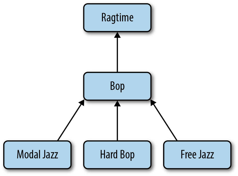
Our schema design will focus on the hierarchy in Figure 5-1. When
designing a hierarchical schema, one approach would be to simply store a
parent_id in each document:
{_id:"modal-jazz",name:"Modal Jazz",parent:"bop",...}
While using such a schema is flexible, it only allows us to examine one level of hierarchy with any given query. If we want to be able to instead query for all ancestors or descendants of a category, it’s better to store the ancestor list in some way.
One approach to this would be to construct the ID of a subcategory based on the IDs of its parent categories:
{_id:"ragtime:bop:modal-jazz",name:"Modal Jazz",parent:"ragtime/bop",...}
This is a convenient approach because:
-
The ancestors of a particular category are self-evident from the
_idfield. -
The descendants of a particular category can be easily queried by using a
prefix-style regular expression. For instance, to find all descendants of
“bop,” you would use a query like
{_id: /^ragtime:bop:.*/}.
There are a couple of problems with this approach, however:
- Displaying the ancestors for a category requires a second query to return the ancestor documents.
-
Updating the hierarchy is cumbersome, requiring string manipulation of the
_idfield.
The solution we’ve chosen here is to store the ancestors as an embedded array,
including the name of each ancestor for display purposes. We’ve also switched to
using ObjectId()s for the _id field and moving the human-readable slug to
its own field to facilitate changing the slug if necessary. Our final schema,
then, looks like the following:
{_id:ObjectId(...),slug:"modal-jazz",name:"Modal Jazz",parent:ObjectId(...),ancestors:[{_id:ObjectId(...),slug:"bop",name:"Bop"},{_id:ObjectId(...),slug:"ragtime",name:"Ragtime"}]}
Operations
This section outlines the category hierarchy manipulations that you may need in an ecommerce site. All examples in this document use the Python programming language and the pymongo driver for MongoDB, but of course you can implement this system using any supported programming language.
Read and display a category
The most basic operation is to query a category hierarchy based on a slug. This type of query is often used in an ecommerce site to generate a list of “breadcrumbs” displaying to the user just where in the hierarchy they are while browsing. The query, then, is the following:
category=db.categories.find({'slug':slug},{'_id':0,'name':1,'ancestors.slug':1,'ancestors.name':1})
In order to make this query fast, we just need an index on the slug field:
>>>db.categories.ensure_index('slug',unique=True)
Add a category to the hierarchy
Suppose we wanted to modify the hierarchy by adding a new category, as shown in
Figure 5-2. This insert operation would be trivial if we had used our
simple schema that only stored the parent ID:
doc = dict(name='Swing', slug='swing', parent=ragtime_id)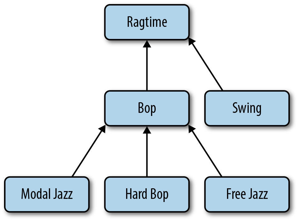
Since we are keeping
information on all the ancestors, however, we need to actually calculate this
array and store it after performing the insert. For this, we’ll define the following
build_ancestors helper function:
defbuild_ancestors(_id,parent_id):parent=db.categories.find_one({'_id':parent_id},{'name':1,'slug':1,'ancestors':1})parent_ancestors=parent.pop('ancestors')ancestors=[parent]+parent_ancestorsdb.categories.update({'_id':_id},{'$set':{'ancestors':ancestors}})
Note that you only need to travel up one level in the hierarchy to get the ancestor list for “Ragtime” that you can use to build the ancestor list for “Swing.” Once you have the parent’s ancestors, you can build the full ancestor list trivially. Putting it all together then, let’s insert a new category:
doc=dict(name='Swing',slug='swing',parent=ragtime_id)swing_id=db.categories.insert(doc)build_ancestors(swing_id,ragtime_id)
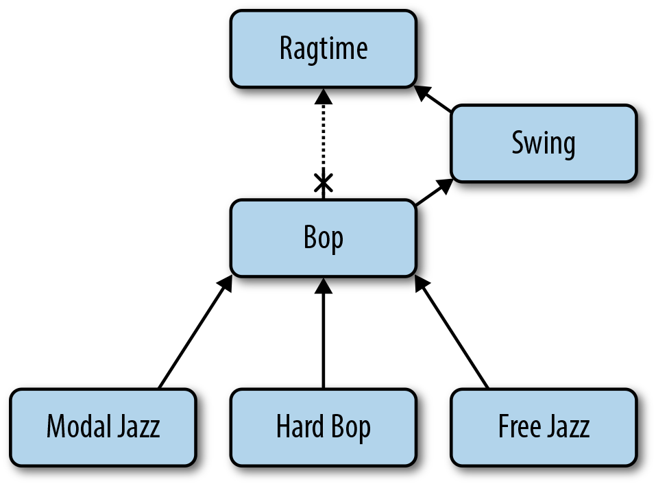
Change the ancestry of a category
This section addresses the process for reorganizing the hierarchy by
moving “Bop” under “Swing,” as shown in Figure 5-3. First, we’ll update
the bop document to reflect the change in its ancestry:
db.categories.update({'_id':bop_id},{'$set':{'parent':swing_id}})
Now we need to update the ancestor list of the bop document and all its
descendants. In order to do this, we’ll first build the subgraph of bop in
memory, including all of the descendants of bop, and then calculate and store
the ancestor list for each node in the subgraph.
For the purposes of calculating the ancestor list, we will store the subgraph in
a dict containing all the nodes in the subgraph, keyed by their parent
field. This will allow us to quickly traverse the hierarchy, starting with the
bop node and visiting the nodes in order:
fromcollectionsimportdefaultdictdefbuild_subgraph(root):nodes=db.categories.find({'ancestors._id':root['_id']},{'parent':1,'name':1,'slug':1,'ancestors':1})nodes_by_parent=defaultdict(list)
forninnodes:nodes_py_parent[n['parent']].append(n)returnnodes_by_parent
-
The
defaultdictfrom the Python standard library is a dictionary with a special behavior when you try to access a key that is not there. In this case, rather than raising aKeyErrorlike a regulardict, it will generate a new value based on a factory function passed to its constructor. In this case, we’re using thelistfunction to create an empty list when the givenparentisn’t found.
Once we have this subgraph, we can update the nodes as follows:
defupdate_node_and_descendants(nodes_by_parent,node,parent):# Update node's ancestorsnode['ancestors']=parent.ancestors+[{'_id':parent['_id'],'slug':parent['slug'],'name':parent['name']}]db.categories.update({'_id':node['_id']},{'$set':{'ancestors':ancestors,'parent':parent['_id']}})# Recursively call children of 'node'forchildinnodes_by_parent[node['_id']]:update_node_and_descendants(nodes_by_parent,child,node)
In order to ensure that the subgraph-building operation is fast, we’ll need an
index on the ancestors._id field:
>>>db.categories.ensure_index('ancestors._id')
Rename a category
One final operation we’ll explore with our category hierarchy is renaming a category. In order to a rename a category, we’ll need to both update the category itself and also update all its descendants. Consider renaming “Bop” to “BeBop,” as in Figure 5-4.
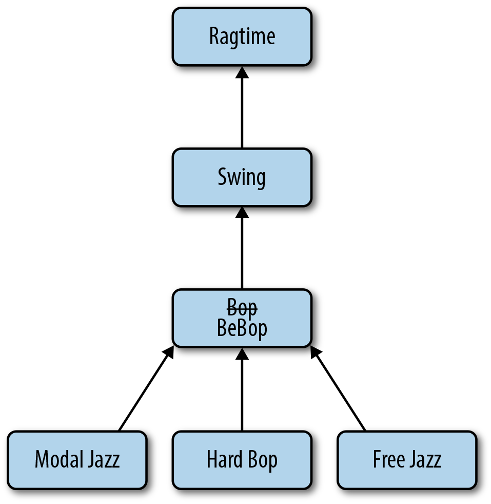
First, we’ll update the category name with the following operation:
db.categories.update({'_id':bop_id},{'$set':{'name':'BeBop'}})
Next, we’ll update each descendant’s ancestors list:
db.categories.update({'ancestors._id':bop_id},{'$set':{'ancestors.$.name':'BeBop'}},multi=True)
There are a couple of things to know about this update:
Sharding Concerns
For most deployments, sharding the categories collection has limited value
because the collection itself will have a small number of documents. If you do
need to shard, since all the queries use _id, it makes an appropriate shard key:
>>>db.command('shardcollection','dbname.categories',{...'key':{'_id':1}}){"collectionsharded":"dbname.categories","ok":1}
Inventory Management
The most basic requirement of an ecommerce system is its checkout functionality. Beyond the basic ability to fill up a shopping cart and pay, customers have come to expect online ordering to account for out-of-stock conditions, not allowing them to place items in their shopping cart unless those items are, in fact, available. This section provides an overview of an integrated shopping cart and inventory management data model for an online store.
Solution Overview
Customers in ecommerce stores regularly add and remove items from their “shopping cart,” change quantities multiple times, abandon the cart at any point, and sometimes have problems during and after checkout that require a hold or canceled order. These activities make it difficult to maintain inventory systems and counts and to ensure that customers cannot “buy” items that are unavailable while they shop in your store.
The solution presented here maintains the traditional metaphor of the shopping cart, but allows inactive shopping carts to age. After a shopping cart has been inactive for a certain period of time, all items in the cart re-enter the available inventory and the cart is emptied. The various states that a shopping cart can be in, then, are summarized in Figure 5-5.
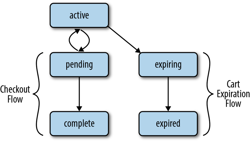
Here’s an explanation of each state:
- active
- In this state, the user is active and items may be added or removed from the shopping cart.
- pending
- In this state, the cart is being checked out, but payment has not yet been captured. Items may not be added or removed from the cart at this time.
- expiring
- In this state, the cart has been inactive for too long and it is “locked” while its items are returned to available inventory.
- expired
- In this state, the shopping cart is inactive and unavailable. If the user returns, a new cart must be created.
Schema
Our schema for this portion of the system consists of two collections:
product and cart. Let’s consider product first. This collection
contains one document for each item a user can place in their cart, called a
“stock-keeping unit” or SKU. The simplest approach is to simply use a SKU
number as the _id and keep a quantity counter for each item. We’ll add in a
details field for any item details you wish to display to the user as they’re
browsing the store:
{_id:'00e8da9b',qty:16,details:...}
It turns out to be useful to augment this schema with a list of shopping carts
containing the particular SKU. We do this because we’re going to use product as
the definitive collection of record for our system. This means that if there is
ever a case where cart and product contain inconsistent data, product is
the collection that “wins.” Since MongoDB does not support multidocument
transactions, it’s important to have a method of “cleaning up” when two
collections become inconsistent, and keeping a carted property in product
provides that avenue here:
{_id:'00e8da9b',qty:16,carted:[{qty:1,cart_id:42,timestamp:ISODate("2012-03-09T20:55:36Z"),},{qty:2,cart_id:43,timestamp:ISODate("2012-03-09T21:55:36Z")}]}
In this case, the inventory shows that we actually have 16 available items, but there are also two carts that have not yet completed checkout, which have one and two items in them, respectively.
Our cart collection, then, would contain an _id, state, last_modified
date to handle expiration, and a list of items and quantities:
{_id:42,last_modified:ISODate("2012-03-09T20:55:36Z"),status:'active',items:[{sku:'00e8da9b',qty:1,details:{...}},{sku:'0ab42f88',qty:4,details:{...}}]}
Note that we’ve copied the item details from the product document into the
cart document so we can display relevant details for each line item without
fetching the original product document. This also helps us avoid the usability
problem of what to do about a SKU that changes prices between being added to the
cart and checking out; in this case, we always charge the user the price at the
time the item was added to the cart.
Operations
This section introduces operations that we’ll want to support on our data model. As always, the examples use the Python programming language and the pymongo driver, but the system can be implemented in any language you choose.
Add an item to a shopping cart
Moving an item from the available inventory to a cart is a fundamental requirement for a shopping cart system. Our system must ensure that an item is never added to a shopping cart unless there is sufficient inventory to fulfill the order.
Patterns
For this operation, and for several others in this section, we’ll use patterns
from Chapter 3 to keep our product and cart collections
consistent.
In order to add an item to our cart, the basic approach will be to:
- Update the cart, ensuring it is still active, and adding the line item.
- Update the inventory, decrementing available stock, only if there is sufficient inventory available.
- If the inventory update failed due to lack of inventory, compensate by rolling back our cart update and raising an exception to the user.
The actual function we write to add an item to a cart would resemble the following:
defadd_item_to_cart(cart_id,sku,qty,details):now=datetime.utcnow()# Make sure the cart is still active and add the line itemresult=db.cart.update({'_id':cart_id,'status':'active'},{'$set':{'last_modified':now},'$push':{'items':{'sku':sku,'qty':qty,'details':details}}})ifnotresult['updatedExisting']:raiseCartInactive()# Update the inventoryresult=db.product.update({'_id':sku,'qty':{'$gte':qty}},{'$inc':{'qty':-qty},'$push':{'carted':{'qty':qty,'cart_id':cart_id,'timestamp':now}}})
ifnotresult['updatedExisting']:# Roll back our cart updatedb.cart.update({'_id':cart_id},{'$pull':{'items':{'sku':sku}}})
raiseInadequateInventory()
-
Here, we’re using the quantity in our
updatespec to ensure that only a document with both the right SKU and sufficient inventory can be updated. Once again, we usesafemode to have the server tell us if anything was updated.-
Note that we need to update the
cartedproperty as well asqtywhen modifyingproduct.-
Here, we
$pullthe just-added item from the cart. Note that$pullmeans that all line items for the SKU will be pulled. This is not a problem for us, since we’ll introduce another function to modify the quantity of a SKU in the cart.
Since our updates always include _id, and this is a unique and indexed field,
no additional indexes are necessary to make this function perform well.
Modifying the quantity in the cart
Often, a user will wish to modify the quantity of a particular SKU in their
cart. Our system needs to ensure that when a user increases the
quantity of an item, there is sufficient inventory. Additionally, the carted
attribute in the product collection needs to be updated to reflect the new
quantity in the cart.
Our basic approach here is the same as when adding a new line item:
- Update the cart (optimistically assuming there is sufficient inventory).
-
Update the
productcollection if there is sufficient inventory. - Roll back the cart update if there is insufficient inventory and raise an exception.
Our code, then, looks like the following:
defupdate_quantity(cart_id,sku,old_qty,new_qty):now=datetime.utcnow()delta_qty=new_qty-old_qty# Make sure the cart is still active and add the line itemresult=db.cart.update({'_id':cart_id,'status':'active','items.sku':sku},{'$set':{'last_modified':now},'$inc':{'items.$.qty':delta_qty}})ifnotresult['updatedExisting']:raiseCartInactive()# Update the inventoryresult=db.product.update({'_id':sku,'carted.cart_id':cart_id,'qty':{'$gte':delta_qty}},{'$inc':{'qty':-delta_qty},'$set':{'carted.$.qty':new_qty,'timestamp':now}})ifnotresult['updatedExisting']:# Roll back our cart updatedb.cart.update({'_id':cart_id,'items.sku':sku},{'$inc':{'items.$.qty':-delta_qty}})
raiseInadequateInventory()
-
Note that we’re including
items.skuin our update spec. This allows us to use the positional$in our$setmodifier to update the correct (matching) line item.-
Both here and in the rollback operation, we’re using the
$incmodifier rather than$setto update the quantity. This allows us to correctly handle situations where a user might be updating the cart multiple times simultaneously (say, in two different browser windows).-
Here again, we’re using the positional
$in our update tocarted, so we need to include thecart_idin our update spec.
Once again, we’re using _id in all our updates, so adding an index doesn’t help
us here.
Checking out
The checkout operation needs to do two main operations:
- Capture payment details.
-
Update the
carteditems once payment is made.
Our basic algorithm here is as follows:
-
Lock the cart by setting it to
pendingstatus. -
Collect payment for the cart. If this fails, unlock the cart by setting it back
to
activestatus. -
Set the cart’s status to
complete. -
Remove all references to this cart from any
cartedproperties in theproductcollection.
The code would look something like the following:
defcheckout(cart_id):now=datetime.utcnow()result=db.cart.update({'_id':cart_id,'status':'active'},update={'$set':{'status':'pending','last_modified':now}})ifnotresult['updatedExisting']:raiseCartInactive()try:collect_payment(cart)except:db.cart.update({'_id':cart_id},{'$set':{'status':'active'}})raisedb.cart.update({'_id':cart_id},{'$set':{'status':'complete'}})db.product.update({'carted.cart_id':cart_id},{'$pull':{'cart_id':cart_id}},multi=True)
-
We’re using the return value from
updatehere to let us know whether we actually locked a currently active cart by moving it to pending status.-
We’re using
multi=Truehere to ensure that all the SKUs that were in the cart have theircartedproperties updated.
Here, we could actually use a new index on the carted.cart_id property so that
our final update is fast:
>>>db.product.ensure_index('carted.cart_id')
Returning inventory from timed-out carts
Periodically, we need to “expire” inactive carts and return their items to available inventory. Our approach here is as follows:
-
Find all carts that are older than the
thresholdand are due for expiration. Lock them by setting their status to"expiring". -
For each
"expiring"cart, return all their items to available inventory. -
Once the
productcollection has been updated, set the cart’s status to"expired".
The actual code, then, looks something like the following:
defexpire_carts(timeout):now=datetime.utcnow()threshold=now-timedelta(seconds=timeout)# Lock and find all the expiring cartsdb.cart.update({'status':'active','last_modified':{'$lt':threshold}},{'$set':{'status':'expiring'}},multi=True)# Actually expire each cartforcartindb.cart.find({'status':'expiring'}):# Return all line items to inventoryforitemincart['items']:db.product.update({'_id':item['sku'],'carted.cart_id':cart['id']},{'$inc':{'qty':item['qty']},'$pull':{'carted':{'cart_id':cart['id']}}})<db.cart.update({'_id':cart['id']},{'$set':{status': 'expired' })
-
We’re using
multi=Trueto “batch up” our cart expiration initial lock.-
Unfortunately, we need to handle expiring the carts individually, so this function can actually be somewhat time-consuming. Note, however, that the
expire_cartsfunction is safely resumable, since we have effectively “locked” the carts needing expiration by placing them in"expiring"status.-
Here, we update the inventory, but only if it still has a
cartedentry for the cart we’re expiring. Note that without thecartedproperty, our function would become unsafe to retry if an exception occurred since the inventory could be incremented multiple times for a single cart.-
Finally, we fully expire the cart. We could also
deleteit here if we don’t wish to keep it around any more.
In order to support returning inventory from timed-out carts, we’ll need to create
an index on the status and last_modified properties. Since our query on
last_modified is an inequality, we should place it last in the compound index:
>>>db.cart.ensure_index([('status',1),('last_modified',1)])
Error handling
The previous operations do not account for one possible failure situation. If an exception occurs after updating the shopping cart but before updating the inventory collection, then we have an inconsistent situation where there is inventory “trapped” in a shopping cart.
To account for this case, we’ll need a periodic cleanup operation that finds
inventory items that have carted items and check to ensure that they exist
in some user’s active cart, and return them to available inventory if they
do not. Our approach here is to visit each product with some carted entry
older than a specified timestamp. Then, for each SKU found:
-
Load the
cartthat’s possibly expired. If it’s actually"active", refresh thecartedentry in theproduct. -
If an
"active"cart was not found to match thecartedentry, then thecartedis removed and the available inventory is updated:
defcleanup_inventory(timeout):now=datetime.utcnow()threshold=now-timedelta(seconds=timeout)# Find all the expiring carted itemsforitemindb.product.find({'carted.timestamp':{'$lt':threshold}}):# Find all the carted items that matchedcarted=dict((carted_item['cart_id'],carted_item)forcarted_iteminitem['carted']ifcarted_item['timestamp']<threshold)# First Pass: Find any carts that are active and refresh the carted# itemsforcartindb.cart.find({'_id':{'$in':carted.keys()},'status':'active'}):cart=carted[cart['_id']]db.product.update({'_id':item['_id'],'carted.cart_id':cart['_id']},{'$set':{'carted.$.timestamp':now}})delcarted[cart['_id']]# Second Pass: All the carted items left in the dict need to now be# returned to inventoryforcart_id,carted_itemincarted.items():db.product.update({'_id':item['_id'],'carted.cart_id':cart_id},{'$inc':{'qty':carted_item['qty']},'$pull':{'carted':{'cart_id':cart_id}}})
-
Here, we’re visiting each SKU that has possibly expired
cartedentries one at a time. This has the potential for being time-consuming, so thetimeoutvalue should be chosen to keep the number of SKUs returned small. In particular, thistimeoutvalue should be greater than thetimeoutvalue used when expiring carts.-
Note that we’re once again using the positional
$to update only thecarteditem we’re interested in. Also note that we’re not just updating theproductdocument in-memory and calling.save(), as that can lead to race conditions.-
Here again we don’t call
.save(), since the product’s quantity may have been updated since this function started executing. Also note that we might end up modifying the sameproductdocument multiple times (once for each possibly expiredcartedentry). This is most likely not a problem, as we expect this code to be executed extremely infrequently.
Here, the index we need is on carted.timestamp to make the initial find() run
quickly:
>>>db.product.ensure_index('carted.timestamp')
Sharding Concerns
If you need to shard the data for this system, the _id field is a reasonable choice
for shard key since most updates use the _id field in their spec, allowing
mongos to route each update to a single mongod process. There are a couple of
potential drawbacks with using _id, however:
-
If the cart collection’s
_idis an increasing value such as anObjectId(), all new carts end up on a single shard. -
Cart expiration and inventory adjustment require update operations and queries
to broadcast to all shards when using
_idas a shard key.
It’s possible to mitigate the first problem at least by using a pseudorandom value for
_id when creating a cart. A reasonable approach would be the following:
importhashlibimportbsondefnew_cart():object_id=bson.ObjectId()cart_id=hashlib.md5(str(object_id)).hexdigest()returncart_id
-
We’re creating a
bson.ObjectId()to get a unique value to use in our hash. Note that sinceObjectIduses the current timestamp as its most significant bits, it’s not an appropriate choice for shard key.-
Now we randomize the
object_id, creating a string that is extremely likely to be unique in our system.
To actually perform the sharding, we’d execute the following commands:
>>>db.command('shardcollection','dbname.inventory'...'key':{'_id':1}){ "collectionsharded" : "dbname.inventory", "ok" : 1 }>>>db.command('shardcollection','dbname.cart')...'key':{'_id':1}){ "collectionsharded" : "dbname.cart", "ok" : 1 }