
Chapter 16
Claims Reserving and IBNR
Markus Gesmann
ChainLadder project
London, United Kingdom
16.1 Introduction
16.1.1 Motivation
The insurance industry, unlike other industries, does not sell products as such, but rather promises. An insurance policy is a promise by the insurer to the policyholder to pay for future claims for an upfront received premium.
As a result, insurers do not know the upfront cost for their service, but rely on historical data analysis and judgment to predict a sustainable price for their offering. In General Insurance (or Non-Life Insurance, e.g. motor, property and casualty insurance); most policies run for a period of 12 months. However, the claims payment process can take years or even decades. Therefore, often not even the delivery date of their product is known to insurers.
In particular, losses arising from casualty insurance can take a long time to settle and even when the claims are acknowledged, it may take time to establish the extent of the claims settlement cost. Claims can take years to materialize. A complex and costly example involves the claims from asbestos liabilities, particularly those in connection with mesothelioma and lung damage arising from prolonged exposure to asbestos. A research report by a working party of the Institute and Faculty of Actuaries estimated that the undiscounted cost of U.K. mesothelioma-related claims to the U.K. Insurance Market for the period 2009 to 2050 could be around £10bn; see Gravelsons et al. (2009). The cost for asbestos-related claims in the United States for the worldwide insurance industry was estimated to be around $120bn in 2002, see Michaels (2002).
Thus, it should come as no surprise that the biggest item on the liabilities side of an insurer's balance sheet is often the provision or reserves for future claims payments. Those reserves can be broken down into case reserves (or outstanding claims), which are losses already reported to the insurance company and losses that are incurred but not reported (IBNR) yet.
Historically, reserving was based on deterministic calculations with pen and paper, combined with expert judgment. Since the 1980s, with the arrival of personal computer, spreadsheet software has become very popular for reserving. Spreadsheets not only reduced the calculation time, but allowed actuaries to test different scenarios and the sensitivity of their forecasts.
As the computer became more powerful, ideas of more sophisticated models started to evolve. Changes in regulatory requirements, for example, Solvency II1 in Europe, have fostered further research and promoted the use of stochastic and statistical techniques. In particular, for many countries, extreme percentiles of reserve deterioration over a fixed time period have to be estimated for the purpose of capital setting.
Over the years, several methods and models have been developed to estimate both the level and variability of reserves for insurance claims; see Schmidt (2012) or P.D. England & R.J. Verrall (2002) for an overview.
In practice, the Mack chain-ladder and bootstrap chain-ladder models are used by many actuaries, along with stress testing / scenario analysis and expert judgment to estimate ranges of reasonable outcomes; see the surveys of U.K. actuaries in 2002, Lyons et al. (2002), and across the Lloyd's market in 2012, Orr (2012).
16.1.2 Outline and Scope
In this chapter we can only give an introduction to some reserving models and the focus will be on the practical implementation in R. For a more comprehensive overview, see Wiitherich & Merz (2008). The remainder of this chapter is structured as follows. Section 16.2 gives an overview of the data structure used for a typical reserving exercise and introduces the example dataset used throughout this chapter. We discuss the classical deterministic chain-ladder reserving method in Section 16.3 and introduce the concept of a tail factor. In Section 16.4 we show first that the chain-ladder algorithm can be considered a weighted linear regression through the origin, and move on from there to introduce stochastic reserving models. We start with the Mack model, which provides a stochastic framework for the chain-ladder methods and allows the estimation of the mean squared error of the payment predictions. Following this, we discuss the Poisson model, a generalised linear model that replicates the chain-ladder forecasts. To estimate the full distribution of the reserve, we consider a bootstrap approach. We finish the section with a log-incremental reserving model that is particularly suited to identify changing trends in the data. Finally, Section 16.5 will briefly discuss the differences between the ultimo and one-year reserve risk measurements in the context of Solvency II.
16.2 Development Triangles
Historical insurance data are often presented in the form of a triangle structure, showing the development of claims over time for each exposure (origin) period. An origin period could be the year the policy was written or earned, or the loss occurrence period. Of course, the origin period does not have to be yearly, for example, quarterly or monthly origin periods are also often used. The development period of an origin period is also called age or lag. Data on the diagonals present payments in the same calendar period. Note: Data of individual policies are usually aggregated to homogeneous lines of business, division levels or perils.
As an example, we present a claims payment triangle from a U.K. Motor Non- Comprehensive account as published by Christofides (1997). For convenience we set the origin period from 2007 to 2013.
The following dataframe presents the claims data in a typical form as it would be stored in a database. The first column holds the origin year, the second column the development year and the third column has the incremental payments / transactions.
> n <- 7
> Claims <- data.frame(originf = factor(rep(2007:2013, n:1)),
+ dev=sequence(n:1),
+ inc.paid=
+ c(3511, 3215, 2266, 1712, 1059, 587,
+ 340, 4001, 3702, 2278, 1180, 956,
+ 629, 4355, 3932, 1946, 1522, 1238,
+ 4295, 3455, 2023, 1320, 4150, 3747,
+ 2320, 5102, 4548, 6283))
To present the data in a triangle format, we can use the matrix function:
> (inc.triangle <- with(Claims, {
+ M <- matrix(nrow=n, ncol=n,
+ dimnames=list(origin=levels(originf), dev=1:n))
+ M[cbind(originf, dev)] <- inc.paid
+ M
+}))
dev
origin 1 2 3 4 5 6 7
2007 3511 3215 2266 1712 1059 587 340
2008 4001 3702 2278 1180 956 629 NA
2009 4355 3932 1946 1522 1238 NA NA
2010 4295 3455 2023 1320 NA NA NA
2011 4150 3747 2320 NA NA NA NA
2012 5102 4548 NA NA NA NA NA
2013 6283 NA NA NA NA NA NA
It is the objective of a reserving exercise to forecast the future claims development in the bottom right corner of the triangle and potential further developments beyond development age 7. Eventually all claims for a given origin period will be settled, but it is not always obvious to judge how many years or even decades it will take. We speak of long and short tail business depending on the time it takes to pay all claims.
Often it is helpful to consider the cumulative development of claims as well, which is presented below:
> (cum.triangle <- t(apply(inc.triangle, 1, cumsum)))
origin 1 2 3 4 5 6 7
2007 3511 6726 8992 10704 11763 12350 12690
2008 4001 7703 9981 11161 12117 12746 NA
2009 4355 8287 10233 11755 12993 NA NA
2010 4295 7750 9773 11093 NA NA NA
2011 4150 7897 10217 NA NA NA NA
2012 5102 9650 NA NA NA NA NA
2013 6283 NA NA NA NA NA NA
The latest diagonal of the triangle presents the latest cumulative paid position of all origin years:
> (latest.paid <- cum.triangle[row(cum.triangle) == n - col(cum.triangle) + 1])
[1] 6283 9650 10217 11093 12993 12746 12690
We add the cumulative paid data as a column to the data frame as well:
> Claims$cum.paid <- cum.triangle[with(Claims, cbind(originf, dev))]
To start the reserving analysis, we plot the data:
> op <- par(fig=c(0,0.5,0,1), cex=0.8, oma=c(0,0,0,0))
> with(Claims, {
+ interaction.plot(x.factor=dev, trace.factor=originf, response=inc.paid,
+ fun=sum, type="b", bty='n', legend=FALSE); axis(1, at=1:n)
+ par(fig=c(0.45,1,0,1), new=TRUE, cex=0.8, oma=c(0,0,0,0))
+ interaction.plot(x.factor=dev, trace.factor=originf, response=cum.paid,
+ fun=sum, type="b", bty='n'), axis(1,at=1:n)
+})
> mtext("Incremental and cumulative claims development",
+ side=3, outer=TRUE, line=-3, cex = 1.1, font=2)
> par(op)
> library(lattice)
> xyplot(cum.paid ~ dev | originf, data=Claims, t="b", layout=c(4,2),
+ as.table=TRUE, main="Cumulative claims development")
Figure 16.1 and Figure 16.2 present the incremental and cumulative claims development by origin year. The triangle appears to be fairly well behaved. The past two years, 2012 and 2013, appear to be slightly higher than years 2008 to 2011, and the values in 2007 are lower in comparison to the later years, for example, the book changed over the years. The last payment of 1,238 for the 2009 origin year stands out a bit as well.
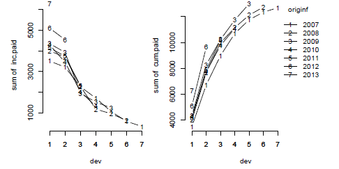
Plot of incremental and cumulative claims payments by origin year using base graphics, using interaction.plot of the stats package in R.

Cumulative claims developments by origin year using the lattice package, with one panel per origin year.
Other claims information can provide valuable insight into the reserving process too, such as claims numbers, transition timings between different claims settlement stages and earning patterns. See, for example, Miranda et al. (2012), Orr (2007), Murray & Lauder (2011), respectively. A deep understanding of the whole business process from pricing, to underwriting, claims handling and data management will guide the actuary to interpret the claims data at hand. The Claims Reserving Working Party Paper, Lyons et al. (2002), outlines the different aspects in more detail.
Notation
Using terminology in Wütherich & Merz (2008), cumulative payments are noted as Ci,j, for origin period i (or period of occurrence) seen after j periods of development and incremental payments Xi,j.. The outstanding liabilities, or reserves, for accident year i at time j is given by
Ri,j=∑k>jXi,j=(limk→∞Ci,k)−Ci,j(16.1)
Because this quantity involves unobserved data (i.e. amounts that will be paid in the future), Ri,j will be the estimated claims reserves.
Remark 16.1 For convenience, we will assume that we work on square matrices, with n rows and n columns. For a more general setting, see Wutherich & Merz (2008).
Remark 16.2 Throughout this chapter we note the first development period as 1. Other authors use 0 for the first development period. This is more a matter of taste than having any practical implications.
Remark 16.3 Many of the methods and models presented here can be applied to paid and reported (often also called 'incurred') data. We either have to estimate the reserve or incurred but not reported (IBNR) claims. For the purpose of this chapter, we assume
Ultimate loss cost |
= paid + reserve |
(16.2) |
= paid + case reserve + IBNR |
(16.3) |
|
= incurred + IBNR |
(16.4) |
Remark 16.4 Some methods and models require data > 0, which for paid claims should be given (insurers rarely receive money back from the insured after a claim was paid2), but case reserves can show negative adjustments over time; therefore incremental incurred triangles do show negatives occasionally. To ensure that data have only positive values, it can be temporarily shifted, or, in a given context, be ignored.
16.3 Deterministic Reserving Methods
The most established and probably oldest method or algorithm for estimating reserves is the so-called chain-ladder method or loss development factor (LDF) method.
The classical chain-ladder method is a deterministic algorithm to forecast claims based on historical data. It assumes that the proportional developments of claims from one development period to the next is the same for all origin periods.
16.3.1 Chain-Ladder Algorithm
Most commonly as a first step, the age-to-age link ratios fk are calculated as the volume weighted average development ratios of a cumulative loss development triangle from one age period to the next Cik for i,k=1,...,n.
fk=∑n−ki=1Ci,k+1∑n−ki=1Ci,k(16.5)
> f <- sapply((n-1):1, function(i) {
sum(cum.triangle[1:i, n-i+1]) / sum(cum.triangle[1:i, n-i])
})
Initially we expect no further development after year 7. Hence, we set the last link ratio (often called the tail factor) to 1:
> tail <- 1
> (f <- c(f, tail))
[1] 1.889 1.282 1.147 1.097 1.051 1.028 1.000
These factors fk are then applied to the latest cumulative payment in each row (Ci,n−i+1) to produce stepwise forecasts for future payment years k∈{n−i+1,...,n}:
ˆCi,k+1=fkˆCi,k,(16.6)
starting with ˆCi,n+1−i=Ci,n+1−i.. The squaring of the claims triangle is calculated below:
> full.triangle <- cum.triangle
> for(k in 1:(n-1)){
full.triangle[(n-k+1):n, k+1] <- full.triangle[(n-k+1):n,k]*f[k]
}
> full.triangle
origin 1 2 3 4 5 6 7
2007 3511 6726 8992 10704 11763 12350 12690
2008 4001 7703 9981 11161 12117 12746 13097
2009 4355 8287 10233 11755 12993 13655 14031
2010 4295 7750 9773 11093 12166 12786 13138
2011 4150 7897 10217 11720 12854 13509 13880
2012 5102 9650 12375 14195 15569 16362 16812
2013 6283 11870 15222 17461 19151 20126 20680
The last column contains the forecast ultimate loss cost:
> (ultimate.paid <- full.triangle[,n])
2007 2008 2009 2010 2011 2012 2013
12690 13097 14031 13138 13880 16812 20680
The cumulative products of the age-to-age development ratios provide the loss development factors for the latest cumulative paid claims for each row to ultimate:
> (ldf <- rev(cumprod(rev(f))))
[1] 3.291 1.742 1.359 1.184 1.080 1.028 1.000
The inverse of the loss development factor estimates the proportion of claims developed to date for each origin year, often also called the gross up factors or growth curve:
> (dev.pattern <- 1/ldf)
[1] 0.3038 0.5740 0.7361 0.8444 0.9261 0.9732 1.0000
The total estimated outstanding loss reserve with this method is
> (reserve <- sum (latest.paid * (ldf - 1)))
[1] 28656
or via
> sum(ultimate.paid - latest.paid)
[1] 28656
Remark 16.5 The basic chain-ladder algorithm has the implicit assumption that each origin period has its own unique level and that development factors are independent of the origin periods; or equivalently, there is a constant payment pattern. Therefore, if ai is the ultimate (cumulative) claim for origin period i and bj is the percentage of ultimate claims in development period j, with ∑bj=1,, then the incremental payment ˆXij can be described as ˆXij=aibj; see Christofides (1997).
> a <- ultimate.paid
> (b <- c(dev.pattern[1], diff(dev.pattern)))
[1] 0.30382 0.27017 0.16208 0.10828 0.08170 0.04716 0.02679
> (X.hat <- a %*% t(b))
[,1] [,2] [,3] [,4] [,5] [,6] [,7]
[1,] 3855 3428 2057 1374 1037 598.4 340.0
[2,] 3979 3538 2123 1418 1070 617.6 350.9
[3,] 4263 3791 2274 1519 1146 661.6 375.9
[4,] 3992 3549 2129 1423 1073 619.5 352.0
[5,] 4217 3750 2250 1503 1134 654.5 371.9
[6,] 5108 4542 2725 1820 1374 792.8 450.4
[7,] 6283 5587 3352 2239 1690 975.2 554.1
Remark 16.6 As the chain-ladder method is a deterministic algorithm and does not regard the observations as realizations of random variables but absolute values, the forecast of the most recent origin periods can be quite unstable. To address this issue, Bornhuetter & Ferguson (1972) suggested a credibility approach, which combines the chain-ladder forecast with prior information on expected loss costs, for example, from pricing data. Under this approach the chain-ladder development to ultimate pattern is used as weighting factors between the pure chain-ladder and expected loss cost estimates.
Suppose the expected loss cost for the 2013 origin year is 20,000; then the BF method, would estimate the ultimate loss cost as
> (BF2013 <- ultimate.paid[n] * dev.pattern[1] + 20000 * (1 - dev.pattern[1]))
2013
20207
16.3.2 Tail Factors
In the previous section we implicitly assumed that there are no claims payment after 7 years, or in other words, that the oldest origin year is fully developed.
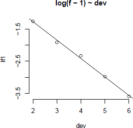
However, often it is not suitable to assume that the oldest origin year is fully settled. A typical approach to overcome this shortcoming is to extrapolate the development ratios, for example, assuming a linear model of the log development ratios minus one, which reflects the incremental changes on the previous cumulative payments; see also Figure 16.3.
> dat <- data.frame(lf1=log(f[-c(1,n)]-1), dev=2:(n-1))
> (m <- lm(lf1 ~ dev , data=dat))
Call:
lm(formula = lf1 ~ dev, data = dat)
Coefficients:
(Intercept) dev
-0.131 -0.572
> plot(lf1 ~ dev, main="log(f - 1) ~ dev", data=dat, bty='n')
> abline(m)
> sigma <- summary(m)$sigma
> extrapolation <- predict(m, data.frame(dev=n:100))
> (tail <- prod(exp(extrapolation + 0.5*sigma"2) +1))
[1] 1.037
We have not carried out any sense checks apart from the plot in Figure 16.3; however, the ratio analysis presented above would suggest that we can expect another 3.7% claims development after year 7 and therefore we should consider increasing our reserve to 29,728.
More generally, the factors used to project the future payments need not always be drawn from the dollar weighted averages of the triangle. Other sources of factors from which the actuary may select link ratios include simple averages from the triangle, averages weighted toward more recent observations or adjusted for outliers, and benchmark patterns based on related, more credible loss experience. Also, because the ultimate value of claims is simply the product of the most current diagonal and the cumulative product of the link ratios, the completion of the interior of the triangle is usually not displayed; instead, the eventual value of the claims, or ultimate value is shown.
For example, suppose the actuary decides that the volume weighted factors from the claims triangle are representative of expected future growth, but discards the tail factor derived from the linear fit in favor of a tail based on data from a larger book of similar business. The LDF method might be displayed in R as follows:
> library(ChainLadder)
> ata(cum.triangle)
origin 1-2 2-3 3-4 4-5 5-6 6-7
2007 1.916 1.337 1.190 1.099 1.050 1.028
2008 1.925 1.296 1.118 1.086 1.052 NA
2009 1.903 1.235 1.149 1.105 NA NA
2010 1.804 1.261 1.135 NA NA NA
2011 1.903 1.294 NA NA NA NA
2012 1.891 NA NA NA NA NA
smpl 1.890 1.284 1.148 1.097 1.051 1.028
vwtd 1.889 1.282 1.147 1.097 1.051 1.028
16.4 Stochastic Reserving Models
As the provision for outstanding claims is often the biggest item on the liabilities side of an insurer's balance sheet, it is important not only to estimate the mean but also the uncertainty of the reserve.
Over the years many statistical techniques have been developed to embed the reserving analysis into a stochastic framework. The key idea is to regard the observed data as one realization of a random variable, rather than absolutes. Statistical techniques also allow for more formal testing, make modelling assumptions more explicit and, in particular, help to monitor actual versus expected claims developments (A versus E). It is the regular A versus E exercise which can help to drive management actions. Hence, as a minimum, not only the mean reserve, or best estimate liabilities3, should be estimated but also the volatility of reserves.
In this section we first show that the deterministic chain-ladder algorithm of the previous section can be considered a weighted linear regression through the origin. Indeed, the following Mack model provides a stochastic framework for the chain-ladder method and allows us to estimate the mean squared error of future payments, using many estimators from the linear regression output. An alternative to the Mack model is the Poisson model, a generalized linear model that replicates the chain-ladder forecasts as well. Yet, the Pois- son model is often not directly applicable to insurance data, as the variance of the data is frequently greater than the mean and hence we consider a quasi-Poisson model to estimate uncertainty metrics. Following this we present a bootstrap technique to estimate the full reserve distribution. For many triangles it is reasonable to assume that the incremental payments follow a log-normal distribution and hence we finish this section with a parametric reserving model that is particularly suited to identify and model changing trends in data.
16.4.1 Chain-Ladder in the Context of Linear Regression
Since the early 1990s, several papers have been published to embed the deterministic chain- ladder method into a statistical framework. Barnett & Zehnwirth (2000) and Murphy (1994) were not the only ones to point out that the chain-ladder age-to-age link ratios could be regarded as coefficients of a linear regression through the origin. To illustrate this concept, we follow Barnett & Zehnwirth (2000).
Let C⋅,k denote the k-th column in the cumulative claims triangle. The chain-ladder algorithm can be seen as
C⋅,k+1=fkC⋅,k+ε(k) with εk~N(0,σ2kCδ⋅,k)(16.7)
The parameter fk describes the slope or the 'best' line through the origin and data points [C⋅,k,C⋅,k+1],, with δ as a 'weighting' parameter. Barnett & Zehnwirth (2000) distinguish the cases:
- δ = 0 ordinary regression with intercept 0
- δ =1 historical chain ladder age-to-age link ratios
- δ = 2 straight averages of the individual link ratios
Indeed, we can demonstrate the different cases by applying different linear models to our data. First, we add columns to the original dataframe Claims, to have payments of the current and previous development period next to each other; additionally we add a column with the development period as a factor.
> names(Claims)[3:4] <- c("inc.paid.k", "cum.paid.k")
> ids <- with(Claims, cbind(originf, dev))
> Claims <- within(Claims,{
cum.paid.kp1 <- cbind(cum.triangle[,-1], NA)[ids]
inc.paid.kp1 <- cbind(inc.triangle[,-1], NA)[ids]
devf <- factor(dev)
}
)
In the next step we apply the linear regression function lm to each development period, vary the weighting parameter δ from 0 to 2 and extract the slope coefficients:
> delta <- 0:2
> ATA <- sapply(delta, function(d)
coef(lm(cum.paid.kp1 ~ 0 + cum.paid.k : devf,
weights=1/cum.paid.k"d, data=Claims))
)
> dimnames(ATA)[[2]] <- paste("Delta = ", delta)
> ATA
Delta = 0 Delta = 1 Delta = 2
cum.paid.k:devf1 1.888 1.889 1.890
cum.paid.k:devf2 1.280 1.282 1.284
cum.paid.k:devf3 1.146 1.147 1.148
cum.paid.k:devf4 1.097 1.097 1.097
cum.paid.k:devf5 1.051 1.051 1.051
cum.paid.k:devf6 1.028 1.028 1.028
Indeed, the development ratios for δ = 1 and δ = 2 tally with those of the previous section. Let us plot the data again, with the cumulative paid claims of one period against the previous one, including the regression output for each development period; see Figure 16.4.
> xyplot(cum.paid.kp1 ~ cum.paid.k | devf,
data=subset(Claims, dev < (n-1)),
main="Age-to-age developments", as.table=TRUE,
scales=list(relation="free"),
key=list(columns=2, lines=list(lty=1:4, type="l"),
text=list(lab=c("lm(y ~ x)",
"lm(y ~ 0 + x)",
"lm(y ~ 0 + x, w=1/x)",
"lm(y ~ 0 + x, w=1/x~2)"))),
panel=function(x,y,...){
panel.xyplot(x,y,...)
if(length(x)>1){
panel.abline(lm(y ~ x), lty=1)
panel.abline(lm(y ~ 0 + x), lty=2)
panel.abline(lm(y ~ 0 + x, weights=1/x), lty=3)
panel.abline(lm(y ~ 0 + x, , weights=1/x"2), lty=4)
}
}
)
Note that for development periods 2 and 3, we observe a difference in the slope of the linear regression with and without an intercept. Of course we could test the significance of the intercept via the usual tests.
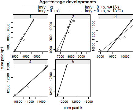
Plot of the cumulative development positions from one development year to the next for each development year, including regression lines of different linear models.
16.4.2 Mack Model
Mack (1993, 1999) suggested a model to estimate the first two moments (mean and standard errors) of the chain-ladder forecast, without assuming a distribution under three conditions.
In order to forecast the amounts ˆCik for k>n+1−i, the Mack chain-ladder model assumes
CL1: ?(Fik|Ci,1,Ci,2,...,Ci,k)=fk with Fik=Ci,k+1Ci,k(16.8)
CL2: Var(Fi,k|Ci,1,Ci,2,...,Ci,k)=σ2kwikCαik(16.9)
CL3: {Ci,1,...,Ci,n},{Cj,1,...,Cj,n}(16.10) are independent for origin period i≠j
with wik∈[0;1],α∈{0,1,2}.. Note that Mack uses the following notation for the weighting parameter α=2−δ,, with δ defined as in the previous section. In other words, the Mack model assumes that the link ratios for each development period are consistent across all origin periods (CL1), the volatility decreases as losses are paid (CL2) and all origi future claims. Thus,
ˆfk=∑n−ki=1wikCαi,kFi,k∑n−ki=1wikCαi,k(16.11)
is an unbiased estimator for fk, given past observations in the triangle, and ˆfk and ˆfj are non-correlated for k≠j. Hence, an unbiased estimator for ?(Ci,k|Ci,1,...,Ci,n+1−i) is
ˆCi,k=ˆfn−1⋅ˆfn−i+1⋅⋅⋅ˆfk−2(ˆfk−1−1)⋅Ci,n+1−i.(16.12)
Recall that ˆfk is the estimator with minimal variance among all linear estimators obtained from the Fi,k's. Finally, if α=1 and wi,k=1, then4.
ˆσ2k=1n−k−1∑n−ki=1(Fi,k−ˆfk)2⋅Ci,k(16.13)
is an unbiased estimator of ˆσ2k , given past observations in the triangle. Based on these estimators, it is possible to compute the mean squared error of prediction for reserve ˆRi, , given past observations ℱ in the triangle
MSEi=^var(ˆRi|ℱ)︸process variance+Ε([Ri−ˆRi]2|ℱ)︸estimation error.(16.14)
The process variance originates from the stochastic movement of the process, whereas the estimation error reflects the uncertainty in the estimation of the parameters.
From Mack (1999) (see also Chapter 3 in Wiitherich & Merz (2008)), the process variance can be estimated using
^Var(ˆRi|ℱ)ˆRin−1∑k=n+1−iˆσ2kˆf2kˆCi,k,(16.15)
and the estimation error estimated by
Ε([Ri−ˆRi]2|ℱ)=ˆR2in−1∑k=n+1−iˆσ2kˆf2k(1Ci,k+1∑n−ki=1Cl,k).(16.16)
In order to derive the conditional mean squared error of total reserve prediction ˆR , define the covariance term, for i<j,, as
MSEi.j+1=ˆC2i,ll∑k=j+2−iˆσ2kˆf2k(1Ci,k+1Σj+1−kl=1Cl,k)+MSEi.j,(16.17)
with MSEi,n+1−i=0. Then the conditional mean squared error of reserves (all years) is
MSE=n∑i=1MSEi+2∑j>iMSEi,j.(16.18)
These formulas are implemented in the ChainLadder package, Gesmann, Murphy & Zhang (2013), via the function MackChainLadder. As an example, we apply the MackChainLadder function5 to our triangle:
> library(ChainLadder)
> (mack <- MackChainLadder(cum.triangle, weights=1, alpha=1,
est.sigma="Mack"))
MackChainLadder(Triangle = cum.triangle, weights = 1, alpha = 1,
est.sigma = "Mack")
i,k
with USEi,n+1—,
Latest Dev.To.Date Ultimate IBNR Mack.S.E CV(IBNR)
2007 12,690 1.000 12,690 0 0.00 NaN
2008 12,746 0.973 13,097 351 3.62 0.0103
2009 12,993 0.926 14,031 1,038 22.90 0.0221
2010 11,093 0.844 13,138 2,045 141.98 0.0694
2011 10,217 0.736 13,880 3,663 426.70 0.1165
2012 9,650 0.574 16,812 7,162 692.39 0.0967
2013 6,283 0.304 20,680 14,39 7 900.58 0.0626
Totals
Latest: 75,672.00
Dev: 0.73
Ultimate:104,327.77
IBN R: 28,655.77
MackS.E.: 1,417.27
CV(IBNR): 0.05
The output provides immediate access to various statistics of the Mack model, including the forecast future payments (here labelled as IBNR), its estimated mean squared error, at individual and across all origin period levels, here ±5%. Hence, the predicted future payments and their errors can be used for an A versus E exercise in the following development period; see Figure 16.5, which was produced using the following command:
> plot(mack, lattice=TRUE, layout=c(4,2))
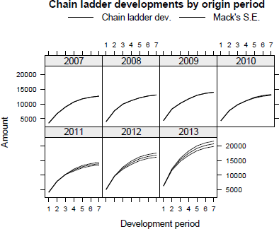
Plot of the actual and expected cumulative claims development and estimated standard error of the Mack model forecast.
To check if the assumptions for the Mack model are held, we review the residual plots of the Mack model; see Figure 16.6.

Plot of MackChainLadder output. The top-left panel shows the latest actual position with the forecasts stacked on top and whiskers indicating the estimated standard error. The top-right panel presents the claims developments to ultimate for each origin year. The four residual plots show the standardized residuals against fitted values, origin, calendar and development period. The residual plots should not show any obvious patterns and about 95% of the standardized residuals should be contained in the range of -2 to 2 for the Mack model to be strictly applicable.
> plot(mack)
From the residual plots we note that smaller values appear under-fitted and larger values slightly over-fitted. The effect of under-fitting appears to be particularly pronounced for data from earlier calendar years, where fewer data are available.
Remark 16.7 One way to address the above shortcomings might be to find appropriate weights and to review the choice of the a parameter in the Mack model. The function CLFMdelta, following Bardis et al. (2012), can help to find consistent a values based on a set of selected age-to-age ratios.
Multivariate Chain-Ladder Models
The Mack chain-ladder technique can be generalized to the multivariate setting where multiple reserving triangles are modelled and developed simultaneously. The advantage of the multivariate modelling is that correlations among different triangles can be modelled, which will lead to more accurate uncertainty assessments.
Reserving methods that explicitly model the between-triangle contemporaneous correlations can be found in Pröhl & Schmidt (2005) and Merz & Wuthrich (2008b).
Another benefit of multivariate loss reserving is that structural relationships between triangles can also be reflected, where the development of one triangle depends on past losses from other triangles. For example, there is generally a need for the joint development of the paid and incurred losses; Quarg & Mack (2004).
Most of the chain-ladder-based multivariate reserving models can be summarised as sequential, seemingly unrelated regressions; Zhang (2010). We note another strand of multivariate loss reserving builds a hierarchical structure into the model to allow estimation of one triangle to borrow strength from other triangles, reflecting the core insight of actuarial credibility; Zhang et al. (2012).
The ChainLadder package provides implementation of multivariate chain-ladder models via the functions MunichChainLadder, MultiChainLadder and MultiChainLadder2. See the package vignette and help files for more details.
16.4.3 Poisson Regression Model for Incremental Claims
Hachemeister & Stanard (1975), Kremer (1982) and finally Mack (1991) examined the validity of treating incremental paid claims as Poisson distributed random variables, noting that the model gives the same forecast as the volume weighted chain-ladder method. Renshaw & Verrall (1998) presented the technique in the context of generalized linear models.
The idea is to assume that incremental payments Xij are Poisson distributed, given the factors origin period ai and development period bj with an intercept c and corner constraints a1=0,b1=0:
log?(Xi,j)=ηi,j=c+ai+bj(16.19)
The Poisson model can be directly implemented via the glm function in R:
> preg <- glm(inc.paid.k ~ originf + devf,
data=Claims, family=poisson(link = "log"))
> summary(preg)
Call:
glm(formula = inc.paid.k ~ originf + devf, family = poisson(link = "log"), data = Claims)
Deviance Residuals:
Min 1Q Median 3Q Max
-7.057 -1.776 0.036 1.675 8.776
Coefficients:
Estimate Std. Error z value Pr(>|z|)
(Intercept) 8.25725 0.01064 776.17 < 2e-16 ***
originf2008 0.03156 0.01263 2.50 0.0124 *
originf2009 0.10042 0.01265 7.94 2.0e-15 ***
originf2010 0.03468 0.01326 2.62 0.0089 **
originf2011 0.08966 0.01367 6.56 5.4e-11 ***
originf2012 0.28129 0.01408 19.98 < 2e-16 ***
originf2013 0.48835 0.01650 29.59 < 2e-16 ***
devf2 -0.11739 0.00914 -12.84 < 2e-16 ***
devf3 -0.62832 0.01170 -53.70 < 2e-16 ***
devf4 -1.03172 0.01498 -68.89 < 2e-16 ***
devf5 -1.31341 0.01910 -68.78 < 2e-16 ***
devf6 -1.86298 0.02991 -62.29 < 2e-16 ***
devf7 -2.42831 0.05527 -43.94 < 2e-16 ***
---
Signif. codes: 0 *** 0.001 ** 0.01 * 0.05 . 0.1 1
(Dispersion parameter for poisson family taken to be 1)
Null deviance: 26197.85 on 27 degrees of freedom
Residual deviance: 322.95 on 15 degrees of freedom
AIC: 615.6
Number of Fisher Scoring iterations: 4
The intercept term estimates the first log-payment of the first origin period. The other coefficients are then additive to the intercept. Thus, the predictor for the second payment of 2008 would be exp(8.25725+0.03156 — 0.11739) = 3538. The second column in the output above gives us immediate access to the standard errors. Other test statistics are provided by summary as well, such as deviance and AIC (see also Chapter 14 for an introduction to the Poisson regression).
Based on those estimated coefficients, we can predict the incremental claims payments as ˆXi,j , but first we have to create a dataframe that holds the future time periods:
> allClaims <- data.frame(origin = sort(rep(2007:2013, n)),
dev = rep(1:n,n))
> allClaims <- within(allClaims, {
devf <- factor(dev)
cal <- origin + dev - 1
originf <- factor(origin)
})
> (pred.inc.tri <- t(matrix(predict(preg,type="response",
newdata=allClaims), n, n)))
[,1] [,2] [,3] [,4] [,5] [,6] [,7]
[1,] 3855 3428 2057 1374 1037 598.4 340.0
[2,] 3979 3538 2123 1418 1070 617.6 350.9
[3,] 4263 3791 2274 1519 1146 661.6 375.9
[4,] 3992 3549 2129 1423 1073 619.5 352.0
[5,] 4217 3750 2250 1503 1134 654.5 371.9
[6,] 5108 4542 2725 1820 1374 792.8 450.4
[7,] 6283 5587 3352 2239 1690 975.2 554.1
The total amount of reserves is the sum of incremental predicted payments for calendar years beyond 2013:
> sum(predict(preg,type="response", newdata=subset(allClaims, cal > 2013)))
> [1] 28656
Observe not only that the total amount of reserves is the same as the chain-ladder method, but also the predicted triangle; see Remark 16.5 on page 550.
From the regression coefficients we can also calculate the chain-ladder age-to-age ratios again:
> df <- c(0, coef(preg)[(n+1):(2*n-1)])
> sapply(2:7, function(i) sum(exp(df[1:i]))/sum(exp(df[1:(i-1)])))
[1] 1.889 1.282 1.147 1.097 1.051 1.028
While it is interesting to assume a Poisson model, since the output is the same as the one obtained using the chain-ladder technique, we have to test if this model is appropriate from a statistical perspective. For instance, assuming equi-dispersion is clearly not valid here:
> library(AER)
> dispersiontest(preg)
Overdispersion test
data: preg
z = 2.966, p-value = 0.001508
alternative hypothesis: true dispersion is greater than 1
sample estimates:
dispersion
11.57
A quasi-Poisson model, with the variance proportional to the mean, should be more reasonable. We will investigate this further in the next section.
Remark 16.8 Note that the so-called Poisson regression — namely glm(Y ..., family= poisson)—can be used on non-integers. Recall that in R, output from a generalised linear- model is obtained using iterated least squares in a standard linear regression on log(Y), if the link function is logarithmic. The only important point in this section is thus to have (strictly) positive incremental payments, not integers; even this can be loosened to the sum of incremental payments for each development period to be positive for a quasi-Poisson model; see P.D. England & R.J. Verrall (2002) and Firth (2003).
Quantifying Uncertainty in GLMs
We continue our analysis with an over-dispersion Poisson model. As mentioned in Kaas et al. (2008), there are closed forms for the variance of any quantity, in generalized linear models. With notations of Chapter 14, in the case of Poisson regression with a logarithmic link function, we have
?(Xi,j|ℱ)=μi,j=exp[ηi,j] and ˆμi,j=exp[ˆηi,j].(16.20)
Using Taylor series expansion, we can approximate Var(ˆxi,j):
Var(ˆxi,j)≈|∂μi,j∂ηi,j|2⋅Var(ˆηi,j),(16.21)
which, with a logarithmic link function, can be simplified to
Thus, the mean squared error of the total amount of reserve is here
With this preparation done we can carry out the regression, assuming a quasi-Poisson distribution:
> summary(odpreg <- glm(inc.paid.k ~ originf + devf, data=Claims,
family=quasipoisson))
Call:
glm(formula = inc.paid.k ~ originf + devf, family = quasipoisson,
data = Claims)
Deviance Residuals:
Min 1Q Median 3Q Max
-7.057 -1.776 0.036 1.675 8.776
Coefficients:
Estimate Std. Error t value Pr(>|t|)
(Intercept) 8.2573 0.0494 166.99 < 2e-16 ***
originf2008 0.0316 0.0587 0.54 0.59861
originf2009 0.1004 0.0588 1.71 0.10819
originf2010 0.0347 0.0616 0.56 0.58185
originf2011 0.0897 0.0635 1.41 0.17850
originf2012 0.2813 0.0654 4.30 0.00063 ***
originf2013 0.4883 0.0767 6.37 1.3e-05 ***
devf2 -0.1174 0.0425 -2.76 0.01452 *
devf3 -0.6283 0.0544 -11.55 7.2e-09 ***
devf4 -1.0317 0.0696 -14.82 2.3e-10 ***
devf5 -1.3134 0.0888 -14.80 2.4e-10 ***
devf6 -1.8630 0.1390 -13.40 9.4e-10 ***
devf7 -2.4283 0.2569 -9.45 1.0e-07 ***
---
Signif. codes: 0 *** 0.001 ** 0.01 * 0.05 . 0.1 1
(Dispersion parameter for quasipoisson family taken to be 21.6)
Null deviance: 26197.85 on 27 degrees of freedom
Residual deviance: 322.95 on 15 degrees of freedom
AIC: NA
Number of Fisher Scoring iterations: 4
Note that the coefficients are the same as for the Poisson model without over-dispersion. However, the dispersion parameter is 21.6 and the errors changed as well. Now we can compute all the components of the mean squared error:
> mu.hat <- predict(odpreg, newdata=allClaims, type="response")*(allClaims$cal>2013)
> phi <- summary(odpreg)$dispersion
> Sigma <- vcov(odpreg)
> model.formula <- as.formula(paste("~", formula(odpreg)[3]))
> # Future design matrix
> X <- model.matrix(model.formula, data=allClaims)
> Cov.eta <- X%*% Sigma %*%t(X)
Hence, the mean squared error is
> sqrt(phi * sum(mu.hat) + t(mu.hat) Cov.eta mu.hat)
[,1]
[1,] 1708
Observe that this is comparable with Mack's mean squared error of 1417.
Nevertheless, the method we just described might not be valid since that expression was obtained using asymptotic theory on generalised linear models, which might not be valid here since we have less than 50 observations.
> op <- par(mfrow=c(2,2), oma = c(0, 0, 3, 0))
> plot(preg)
> par(op)
Warning messages:
1: not plotting observations with leverage one:
7, 28
2: not plotting observations with leverage one:
7, 28
Still, the residual plots, see Figure 16.7, look reasonable, but R gives us a warning in respect of two data points that have a leverage greater than one. Lines 7 and 28 refer to the development years 2 and 1 for the origin years 2009 and 2013 respectively.
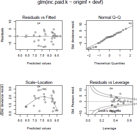
The output of the Poisson model appears to be well behaved. However, the last plot produces a warning that should be investigated.
Indeed, the first payment in 2013 is considerably higher than those in previous years and also the payment for the 2009 year after 24 months is higher in relation to the payment in year 3. Again, this should prompt further investigations into the data.
Remark 16.9 A wider range of generalized reserving models is provided in the ChainLadder package via the function glmReserve. It takes origin period and development period as mean predictors in estimating the ultimate loss reserves, and provides both analytical and bootstrapping methods to compute the associated prediction errors. The bootstrapping approach also generates the full predictive distribution for loss reserves. To replicate the results of this section we use:
> (odp <- glmReserve(as.triangle(inc.triangle), var.power=1, cum=FALSE))
Latest Dev.To.Date Ultimate IBNR S.E CV
2008 12746 0.9732 13097 351 125.8 0.35843
2009 12993 0.9260 14031 1038 205.1 0.19757
2010 11093 0.8443 13138 2045 278.9 0.13636
2011 10217 0.7361 13880 3663 386.8 0.10559
2012 9650 0.5740 16812 7162 605.3 0.08451
2013 6283 0.3038 20680 14397 1158.1 0.08044
total 62982 0.6873 91638 28656 1708.2 0.05961
Remark 16.10 The use of generalised linear models in insurance loss reserving has many compelling aspects; for example,
- When the over-dispersed Poisson model is used, it reproduces the estimates from the chain-ladder method.
- It provides a more coherent modelling framework than the Mack model.
- All the relevant established statistical theory can be directly applied to perform hypothesis testing and diagnostic checking.
However, the user should be cautious of some of the key assumptions that underlie the generalised linear model, in order to determine whether this model is appropriate for the problem considered:
- The generalised linear model assumes no tail development, and it only projects losses to the latest time point of the observed data. To use a model that enables tail extrapolation, consider the growth curve model ClarkLDF or ClarkCapeCod in the ChainLadder package; see also Clark (2003).
- The model assumes that each incremental loss is independent of all the others. This assumption may not be valid, in that cells from the same calendar year are usually correlated due to inflation or business operating factors (e.g. catastrophe losses can effect policies from multiple origin periods).
- The model tends to be over-parametrized, which may lead to inferior predictive performance.
16.4.4 Bootstrap Chain-Ladder
An alternative to asymptotic econometric relationships can be to use the bootstrap methodology. Here we present a two-stage simulation approach, following P.D. England & R.J. Verrall (2002).
In the first stage, a quasi-Poisson model is applied to the claims triangle to forecast future payments. From this we calculate the scaled-Pearson residuals, assuming that they are approximately independent and identical distributed. These residuals are re-sampled with replacement many times to generate bootstrapped (pseudo) triangles and to forecast future claims payments to estimate the parameter error. Recall that the predictions of the quasi-Poisson model are the same as those from the chain-ladder method, hence we use the latter faster algorithm.
In the second stage, we simulate the process error with the bootstrap value as the mean and an assumed process distribution, here a quasi-Poisson. The set of reserves obtained in this way forms the predictive distribution, from which summary statistics such as mean, prediction error or quantiles can be derived.
In a Poisson regression, the Pearson's residuals are
In order to have a proper estimator of the variance (to have residuals with unit variance), we have to adjust the residuals for the number of regression parameters k (i.e. 2n — 1) and observations n:
The strategy is to bootstrap among those residuals to get a sample and to generate a pseudo triangle
Then we can use standard techniques to complete the triangle, and extrapolate the lower part. As mentioned in the introduction to Mack's approach, there are two kinds of uncertainty: uncertainty in the estimation of the model, and uncertainty in the process of future payments.
If we use the predictions from a quasi-Poisson model in this new triangle, we will predict the expected value of future payments. In order to quantify uncertainty, it is necessary to generate scenarios of payments.
This two-stage bootstrapping/simulation approach is implemented in the BootChainLadder function as part of the ChainLadder package.
As input parameters we provide the cumulative triangle, the number of bootstraps and the process distribution to be assumed:
> set.seed(1)
> (B <- BootChainLadder(cum.triangle, R=1000, process.distr="od.pois"))
 BootChainLadder(Triangle = cum.triangle, R = 1000, process.distr = "od.pois")
Latest Mean Ultimate Mean IBNR SD IBNR IBNR 75% IBNR 95%
2007 12,690 12,690 0 0 0 0
2008 12,746 13,099 353 127 430 569
2009 12,993 14,025 1,032 202 1,165 1,368
2010 11,093 13,133 2,040 270 2,216 2,525
2011 10,217 13,866 3,649 392 3,900 4,336
2012 9,650 16,815 7,165 630 7,559 8,268
2013 6,283 20,677 14,394 1,185 15,203 16,298
Totals
Latest: 75,672
Mean Ultimate: 104,305
Mean IBNR: 28,633
SD IBNR: 1,721
Total IBNR 75%: 29,787
Total IBNR 95%: 31,312
The first two moments are, not surprisingly, similar to the Poisson model. In contrast to the Mack model, which only provides the first two moments for the underlying distributions, here we have also access to the various percentiles of the estimated distribution of future payments.
The default plot of the model output, see Figure 16.8, presents the distribution of the simulated future payments (here labelled IBNR) and an initial sense check of the model by comparing the latest actual payments against simulated data.

The top-left chart shows a histogram of the simulated future payments (here labelled IBNR) across all origin years. The line chart in the top right presents the empirical cumulative distribution of those simulated future payments. The bottom row shows a breakdown by origin year. The first box-whisker plot on the left displays the simulations by year, with the mean highlighted as a dot. The box-whisker plot to the right can be used to test the model, as it shows the latest actual claim for each origin year against the simulated distribution.
>
  plot(B)
For capital setting purposes, it is desirable to look at the extreme percentiles of the simulated data. The BootChainLadder function also gives us access to the simulated triangles, which allows us to extract percentiles using the quantile function:
> quantile(B, c(0.75,0.95,0.99, 0.995))
$ByOrigin
IBNR 75% IBNR 95% IBNR 99% IBNR 99.5%
2007 0 0.0 0 0.0
2008 430 569.1 716 746.2
2009 1165 1368.2 1514 1580.2
2010 2216 2525.0 2757 2809.4
2011 3900 4336.1 4641 4803.1
2012 7559 8268.0 8858 9014.0
2013 15203 16298.3 17215 17482.1
$Totals
Totals
IBNR 75%: 29787
IBNR 95%: 31312
IBNR 99%: 32859
IBNR 99.5%: 33278
For many lines of business in non-life insurance, it is not unreasonable that losses follow a lognormal distribution. We can test this idea for our data by fitting a log-normal distribution to the predicted future payments. The fitdistrplus package by Delignette-Muller et al. (2013) makes it a one liner in R:
> library(fitdistrplus)
> (fit <- fitdist(B$IBNR.Totals[B$IBNR.Totals>0], "lnorm"))
Fitting of the distribution ' lnorm ' by maximum likelihood Parameters:
estimate Std. Error
meanlog 10.26051 0.001908
sdlog 0.06033 0.001347
> plot(fit)
The fit looks very reasonable indeed, see Figure 16.9, and the 99.5 percentile of the fitted log-normal is close to the sample percentile above:

> qlnorm(0.995, fit$estimate['meanlog'], fit$estimate['sdlog'])
[1] 33387
Payment distribution over the next year
As we have access to all simulated triangles, we can also estimate percentiles for payments in the following year. For the 99.5 percentile payment over the next 12 months, we get
> ny <- (col(inc.triangle) == (nrow(inc.triangle) - row(inc.triangle) + 2))
> paid.ny <- apply(B$IBNR.Triangles, 3,
function(x){
next.year.paid <- x[col(x) == (nrow(x) - row(x) + 2)] sum(next.year.paid)
})
> paid.ny.995 <- B$IBNR.Triangles[,,order(paid.ny)[round(B$R*0.995)]]
> inc.triangle.ny <- inc.triangle
> (inc.triangle.ny[ny] <- paid.ny.995[ny])
[1] 7076 3308 1352 970 868 338
This would reflect a 49% reserve utilisation over the next year (sum of payments next year devided by total reserve).
16.4.5 Reserving Based on Log-Incremental Payments
We noted in the previous section that the claims appear to follow a log-normal distribution. Zehnwirth (1994) was not the first to consider modelling the log of the incremental claims payments, but his papers and software ICRFS6 have popularised this approach. Here we present the key concepts of what Zehnwirth (1994) calls the probabilistic trend family (PTF).
Zehnwirth's model assumes the following structure for the incremental claims :
The errors are assumed to be normal with . The parameters model trends in three time directions, namely origin year, development year and calendar (or payment) year, respectively; see Figure 16.10.

Structure of a typical claims triangle and the three time directions: origin, development, and calendar periods.
Christofides (1997) examines a very similar model, but uses the following notation:
with a, d representing the parameters in origin and development period direction (a parameter for the payment year direction could be added). Although the models in Equations (16.27) and (16.28) are essentially the same, the design matrices differ and therefore the coefficients and their interpretation.
Remark 16.11 Note that the above model is not a GLM, that is, . Instead, it models , although both models assume . Hence, we will use least squares regression to fit the coefficients via lm again.
Before we apply the log-linear model to the data, and we will follow Christofides (1997), we shall plot it again on a log-scale.
> Claims <- within(Claims, {
log.inc <- log(inc.paid.k)
cal <- as.numeric(levels(originf))[originf] + dev - 1
})
The interaction plot, Figure 16.11, suggests a linear relationship after the second development year on a log-scale. The lines of the different origin years are fairly closely grouped, but the last 2 years, labelled 6 and 7, do stand out. We shall test if this is significant. We start with a model using all levels of the origin factor and two dummy parameters for the development year, with d27 for . Hence, we add two dummy variables to our data:

The interaction plot shows the developments of the origin years on a log-scale. From the second development year, the decay appears to be linear.
> Claims <- within(Claims, {
d1 <- ifelse(dev < 2, 1, 0)
d27 <- ifelse(dev < 2, 0, dev - 1)
})
The dummy variable d1 is 1 for the first development period and 0 otherwise, while d27 is 0 for the first development period and counts up from 1 then onwards. Hence, we will estimate one parameter for the first payment and a constant trend (decay) for the following periods:
> summary(fit1 <- lm(log.inc ~ originf + d1 + d27, data=Claims))
Call:
lm(formula = log.inc ~ originf + d1 + d27, data = Claims)
Residuals:
Min 1Q Median 3Q Max
-0.2214 -0.0397 0.0112 0.0329 0.1962
Coefficients:
Estimate Std. Error t value Pr(>|t|)
(Intercept) 8.572835 0.075690 113.26 < 2e-16 ***
originf2008 0.000956 0.063935 0.01 0.98822
originf2009 0.092037 0.068675 1.34 0.19600
originf2010 -0.018715 0.075261 -0.25 0.80629
originf2011 0.063828 0.084302 0.76 0.45825
originf2012 0.272668 0.098245 2.78 0.01205 *
originf2013 0.468983 0.131593 3.56 0.00207 **
d1 -0.296215 0.069903 -4.24 0.00045 ***
d27 -0.434960 0.018488 -23.53 1.6e-15 ***
---
Signif. codes: 0 *** 0.001 ** 0.01 * 0.05 . 0.1 1
Residual standard error: 0.114 on 19 degrees of freedom
Multiple R-squared: 0.983, Adjusted R-squared: 0.976
F-statistic: 139 on 8 and 19 DF, p-value: 3.29e-15
The model output confirms what we had noticed from the interaction plot already; apart from the origin years 2012 and 2013 there is no significant difference between the years; the p-values are all greater than 5% and the coefficients are less than twice their standard errors.
Therefore we reduce the model and replace the origin variable with two dummy columns for those years:
> Claims <- within(Claims, {
a6 <- ifelse(originf == 2012, 1, 0)
a7 <- ifelse(originf == 2013, 1, 0)
})
> summary(fit2 <- lm(log.inc ~ a6 + a7 + d1 + d27, data=Claims))
Call:
lm(formula = log.inc ~ a6 + a7 + d1 + d27, data = Claims)
Residuals:
Min 1Q Median 3Q Max
-0.21567 -0.04910 0.00654 0.05137 0.27199
Coefficients:
Estimate Std. Error t value Pr(>|t|)
(Intercept) 8.6079 0.0515 167.14 < 2e-16 ***
a6 0.2435 0.0852 2.86 0.00887 **
a7 0.4411 0.1217 3.62 0.00142 **
d1 -0.3035 0.0678 -4.48 0.00017 ***
d27 -0.4397 0.0167 26.39 < 2e-16 ***
Signif. codes: 0 *** 0.001 ** 0.01 * 0.05 . 0.1 1
---
Residual standard error: 0.112 on 23 degrees of freedom
Multiple R-squared: 0.98, Adjusted R-squared: 0.977
F-statistic: 288 on 4 and 23 DF, p-value: <2e-16
The reduction in parameters from 9 to 5 seems sensible, all coefficient are significant and the model error reduced from 0.114 to 0.112 as well. Further we can read off the coefficient for d27 that claims payments are predicted to reduce by 44% each year after year 1. Next, we plot the model:
> op <- par(mfrow=c(2,2), oma = c(0, 0, 3, 0))
> plot(fit2)
> par(op)
Reviewing the residual plots in Figure 16.12 highlights again the latest payment for the 2009 origin year (the 18th row of the Claims data) as a potential outlier.

Residual plots of the log-incremental model fit2. The last payment of 2009 (row 18) is highlighted again as a potential outlier, and so are rows 4, 7 and 11.
The error distribution appears to follow a normal distribution, top right QQ-plot in Figure 16.12, confirmed by the Shapiro-Wilk normality test:
> shapiro.test(fit2$residuals)
Shapiro-Wilk normality test
data: fit2$residuals
W = 0.9654, p-value = 0.4638
To investigate the residuals further, we shall plot them against the fitted values and the three trend directions. The following function will create those four plots for our model.
> resPlot <- function(model, data){
xvals <- list(
fitted = model[['fitted.values']],
origin = as.numeric(levels(data$originf))[data$originf],
cal=data$cal, dev=data$dev
)
op <- par(mfrow=c(2,2), oma = c(0, 0, 3, 0))
for(i in 1:4){
plot.default(rstandard(model) ~ xvals[[i]] ,
main=paste("Residuals vs", names(xvals)[i]),
xlab=names(xvals)[i], ylab="Standardized residuals")
panel.smooth(y=rstandard(model), x=xvals[[i]])
abline(h=0, lty=2)
}
mtext(as.character(model$call)[2], outer = TRUE, cex = 1.2)
par(op)
}
> resPlot(fit2, Claims)
Again, the residual plots all look fairly well behaved; however, we notice from the bottom-left plot in Figure 16.13 that claims for the payment years 2007, 2008 are slightly over-fitted and 2009, 2010 are under-fitted. Hence, we introduce an additional parameter for that period and update our model:
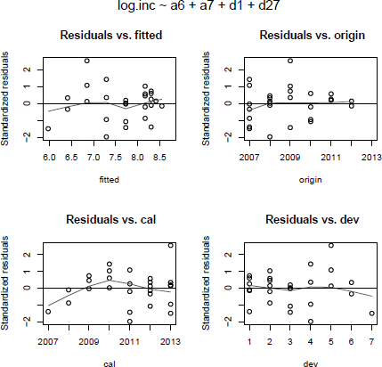
Residual plots of the log-incremental model fit2 against fitted values and the three trend directions.
> Claims <- within(Claims, {
p34 <- ifelse(cal < 2011 & cal > 2008, cal-2008, 0)
})
> summary(fit3 <- update(fit2, ~ . + p34, data=Claims))
Call:
lm(formula = log.inc ~ a6 + a7 + d1 + d27 + p34, data = Claims)
Residuals:
Min 1Q Median 3Q Max
-0.1941 -0.0595 0.0164 0.0511 0.2840
Coefficients:
Estimate Std. Error t value Pr(>|t|)
(Intercept) 8.5576 0.0540 158.51 < 2e-16 ***
a6 0.2822 0.0819 3.45 0.00230 **
a7 0.4777 0.1152 4.15 0.00042 ***
d1 -0.2897 0.0638 -4.54 0.00016 ***
d27 -0.4301 0.0163 -26.45 < 2e-16 ***
p34 0.0603 0.0292 2.07 0.05074 .
---
Signif. codes: 0 *** 0.001 ** 0.01 * 0.05 . 0.1 1
Residual standard error: 0.105 on 22 degrees of freedom
Multiple R-squared: 0.984, Adjusted R-squared: 0.98
F-statistic: 264 on 5 and 22 DF, p-value: <2e-16
> resPlot(fit3, Claims)
The residual plot against calendar years, Figure 16.14, has improved and the parameter p34 could be regarded significant. The coefficient p34 describes a 6% increase of claims payments in those 2 years. An investigation should clarify if this effect is the result of a temporary increase in claims inflation, a change in the claims settling process, other causes or just random noise. Observe that the new model has a slightly lower residual standard error of 0.105 compared to 0.112.

Within the linear regression framework we can forecast the claims payments and estimate the standard errors. We follow the paper by Christofides (1997) again. Recall that for a lognormal distribution, the mean is and the variance is where are the mean and standard deviation of the logarithm, respectively
> log.incr.predict <- function(model, newdata){
Pred <- predict(model, newdata=newdata, se.fit=TRUE)
Y <- Pred$fit
VarY <- Pred$se.fit"2 + Pred$residual.scale"2
P <- exp(Y + VarY/2)
VarP <- P~2*(exp(VarY)-1)
seP <- sqrt(VarP)
model.formula <- as.formula(paste("~", formula(model)[3]))
mframe <- model.frame(model.formula, data=newdata)
X <- model.matrix(model.formula, data=newdata)
varcovar <- X %*% vcov(model) %*% t(X)
CoVar <- sweep(sweep((exp(varcovar)-1), 1, P, "*"), 2, P, "*")
CoVar[col(CoVar)==row(CoVar)] <- 0
Total.SE <- sqrt(sum(CoVar) + sum(VarP))
Total.Reserve <- sum(P)
Incr=data.frame(newdata, Y, VarY, P, seP, CV=seP/P)
out <- list(Forecast=Incr,
Totals=data.frame(Total.Reserve,
Total.SE=Total.SE,
CV=Total.SE/Total.Reserve))
return(out)
}
With the above function it is straightforward to carry out the prediction for future claims payment and standard errors. As a bonus we can estimate payments beyond the available data.
To forecast the future claims, we prepare a data frame with the predictors for those years, here with 6 years beyond age 7:
> tail.years <-6
> fdat <- data.frame(
origin=rep(2007:2013, n+tail.years),
dev=rep(1:(n+tail.years), each=n)
)
> fdat <- within(fdat, {
cal <- origin + dev - 1
a7 <- ifelse(origin == 2013, 1, 0)
a6 <- ifelse(origin == 2012, 1, 0)
originf <- factor(origin)
p34 <- ifelse(cal < 2011 & cal > 2008, cal-2008, 0)
d1 <- ifelse(dev < 2, 1, 0)
d27 <- ifelse(dev < 2, 0, dev - 1)
})
So, here are the results for the two models:
> reserve2 <- log.incr.predict(fit2, subset(fdat, cal>2013))
> reserve2$Totals
Total.Reserve Total.SE CV
1 33847 2545 0.07519
> reserve3 <- log.incr.predict(fit3, subset(fdat, cal>2013))
> reserve3$Totals
Total.Reserve Total.SE CV
1 34251 2424 0.07078
The two models produce very similar results and it should not be much of a surprise as they are quite similar indeed. The third model has proportionally a slightly smaller standard error and may hence be the preferred choice.
The future payments can be displayed with the xtabs function:
> round(xtabs(P ~ origin + dev, reserve3$Forecast))
dev
origin 2 3 4 5 6 7 8 9 10 11 12 13
2007 0 0 0 0 0 0 259 168 110 71 47 30
2008 0 0 0 0 0 397 259 168 110 71 47 30
2009 0 0 0 0 610 397 259 168 110 71 47 30
2010 0 0 0 937 610 397 259 168 110 71 47 30
2011 0 0 1441 937 610 397 259 168 110 71 47 30
2012 0 2946 1916 1247 812 529 344 224 146 95 62 40
2013 5529 3595 2338 1521 990 645 420 273 178 116 76 49
The model structure is clearly visible in the above future claims triangle; as the origin years 2007 to 2011 share the same parameter, the predicted future payments for those years have the same identical mean expectations.
For comparison, here is the output of the Mack chain-ladder model, assuming a tail factor of 1.05 and standard error of 0.02:
> round(summary(MackChainLadder(cum.triangle, est.sigma="Mack",
tail=1.05, tail.se=0.02))$Totals,2)
Totals
Latest: 75672.00
Dev: 0.69
Ultimate: 109544.16
IBNR: 33872.16
Mack S.E.: 2563.40
CV(IBNR): 0.08
The chain-ladder method provides a forecast similar to the log-incremental regression model, but at the price of many more parameters and hence potential instability.
A model with few parameters is potentially more robust and can be analysed by back testing the model with fewer data points.
The log-incremental regression model provides an intuitive and elegant stochastic claims reserving model and can help to investigate trends in the calendar/payment year direction, such as claims inflation, which is challenging to define and measure; Gesmann, Rayees & Clapham (2013). Additionally, the tail extrapolation is part of the model design and not an artificial add-on.
See Christofides (1997) and Zehnwirth (1994) for a more detailed discussion of the log-incremental model.
16.5 Quantifying Reserve Risk
The most frequent reason insurance companies failed in the past was insufficient reserves; Massey et al. (2002). Hence, as mentioned earlier, monitoring claims development is one of main purposes of the models presented in the previous section. Models, unlike deterministic point estimators, allow the actuary to judge the materiality of payment deviation from modelled expected claims development.
Yet, we have to acknowledge that a model cannot be proven right, or, to put it more bluntly: You make money, until you don't.
Therefore it is important to understand the underlying model assumptions and to quantify the uncertainty of the predicted mean ultimate loss costs. Typical risk measures are mean squared error, value at risk (VaR) and tail value at risk (TVaR). These risk metrics can be defined over different time horizons and play a key role in assessing capital requirements for reserve risk.
16.5.1 Ultimo Reserve Risk
The uncertainty around the ultimate loss cost, also called ultimo reserve risk, estimates the risk that the reserve is not sufficient to cover claims payments for the full run-off of today's liabilities. It is an important metric for capital setting and when pricing the transfer of run-off books of business and has been in use for many years.
Estimators for the ultimo risk were given for all the stochastic reserving models of the previous section. The log-incremental and bootstrap models provide direct access to various percentiles, while the Mack model only provides estimation for the mean and mean squared error and hence requires a distribution assumption, for example, log-normal to estimate extreme percentiles.
16.5.2 One-Year Reserve Risk
The reserve risk over a 1-year time horizon measures the change required in the estimate of ultimate loss cost conditioned on the claims development over the following year. This metric is used to assess the reserve risk under the proposed Solvency II regime.
The Solvency II framework is consistent with a mark to market basis, and therefore focuses on the 1-year view of the balance sheet, which requires the discounting of future cash flows based on an assumed interest rate(s). Reserve risk is specifically defined as the difference between the best estimate reserve at t = 0 and after 12 months (t = 1), following claims deterioration or a claims shock with 0.5% probability.
Merz & Wuthrich (2008a) analysed the Mack model and derived analytical formulas for the claims development result (CDR). Ohlsson & Lauzeningks (2009) also described a simulation approach to quantify the 1-year risk.
Estimating the 1-year reserve risk can be computationally demanding, and many aspects such as the inclusion of expert judgement and tail factors are fields of active research.
Remark 16.12 Similar ideas to the 1-year reserve risk are applied to back test reserving models. By removing the latest calendar year data from a claims triangle and comparing its prediction with the forecast based on the complete data, we can test the robustness of the model and its parameters.
Illustrative 1-year reserve risk example
To clarify the concept, we present an illustrative example of how to estimate the 1-year reserve risk. We follow the ideas of Felisky et al. (2010) and simplify those even further.
From our bootstrap model we extracted the future claims triangle that has shown the highest payment in the following calendar year at the 99.5 percentile, see page 567. We add the shock payment of the next year to the original triangle and re-forecast the extended triangle to ultimate, using the chain-ladder algorithm (note that the age-to-age link ratios will change, but no tail factor is assumed), and compare the newly predicted reserve with the original forecast.
origin 1 2 3 4 5 6 7
2007 3511 6726 8992 10704 11763 12350 12690
2008 4001 7703 9981 11161 12117 12746 13084
2009 4355 8287 10233 11755 12993 13861 NA
2010 4295 7750 9773 11093 12063 NA NA
2011 4150 7897 10217 11569 NA NA NA
2012 5102 9650 12958 NA NA NA NA
2013 6283 13359 NA NA NA NA NA
> f.ny <- sapply((n-1):1, function(i){
sum(cum.triangle.ny[1:(i+1), n-i+1])/sum(cum.triangle.ny[1:(i+1), n-i])
})
> (f.ny <- c(f.ny[-(n-1)],1))
[1] 1.936 1.295 1.144 1.094 1.057 1.000
> full.triangle.ny <- cum.triangle.ny
> for(k in 2:(n-1)){
full.triangle.ny[(n-k+2):n, k+1] <- full.triangle.ny[(n-k+2):n,k]*f[k]
}
> (sum(re.reserve.995 <- full.triangle.ny[,n] - rev(latest.paid)))
[1] 31951
We observe that after a 1 in 200 payment shock year, the reserve would increase from 28,656 to 31,951 (+11%). Therefore the one-year reserve risk is 3,295, assuming that the actuary would not change further assumptions.
To put this metric into context, suppose the reserve is twice the volume of net earned premiums in the following year; then this would suggest a prior year deterioration of 22% on the combined ratio.
This simplified re-reserving approach has of course its limitation; it is only a point estimator. The payment shock movement is purely dependent on the historical data volatility and cannot capture events such as changes in legislation or other exogenous influences.
Note that the reserve after the 1-year shock development is less than the predictions that include a tail factor. This demonstrates that estimating the 1-year reserve risk is far more complex than illustrated with the toy example above and that the actuary would have to consider carefully how she would re-reserve the same book of business in the following year, that is, she may want to re-consider trends in the calendar year direction.
In reality, if we had a massive spike in paid losses, unless this related to a single claim, which seems unlikely at the 1 in 200 level, chances are we have issues in many areas. Therefore we will probably cross check claims with material case reserves and review them as well. The influence of case reserves is ignored in this example.
Remark 16.13 Long tail classes of business may have a lower reserve risk over a 1-year horizon than short tail lines of business. Their claims development can be much slower and hence changes can take longer to materialize.
On the other hand, it is also more difficult to detect reserve deterioration for long tail lines. Exemplified in the past, by the soft U.S.-casualty cycle of the late 1990s that showed prior year deteriorations reported over several years.
16.6 Discussion
This chapter gave a brief overview of how some of the more popular claims reserving methods and models can be applied in R. For more details about the models and their mathematical derivation, see the original papers, Wütherich & Merz (2008) or Kaas et al. (2008).
Claims reserving is a complex and evolving subject. Changes in regulation, e.g. Solvency II in Europe, are expected to accelerate the adoption of stochastic reserving frameworks. Although the Mack and Bootstrap models, which are simple to implement in spreadsheet software, are popular with actuaries today, we demonstrated that many other stochastic models are straightforward to apply in a statistical environment such as R.
There are many other aspects that need to be considered in a full reserving analysis and which were not covered here; to name but a few:
- Claims inflation and other exogenous influences such as legislation, social environment, climate change
- Changes in business processes, earning patterns, accounting practice and data quality in general
- Changes to exposure and underlying policy terms and conditions
- Aggregation of reserves across multiple lines of business
- Treatment of large and catastrophic losses
- Treatment of reinsurance
Reserving is always mixture of art and science, and requires a combination of sound data analysis with business knowledge and judgement. In this sense, a Bayesian approach would lead naturally to the inclusion of expert judgement and the full reserve distribution.
Using hierarchical or multilevel models as presented by Guszcza (2008) appears a natural next step for claims reserving. The Clark LDF model, Clark (2003), mentioned by Guszcza (2008), has already been implemented by Daniel Murphy in R as part of the ChainLadder package. Additionally, the double-chain-ladder approach of Miranda et al. (2012) looks like a promising extension of the chain-ladder family of models.
Also worth mentioning is the lossDev package by Laws & Schmid (2012) that implements robust loss development using Markov Chain Monte Carlo (MCMC) using rjags, Plummer (2013).
So, which reserving model should I use?
It depends. Unfortunately, there is no easy answer.
It depends on the data, the context, the type of business, the tail characteristic, the time available, your statistical knowledge and, of course, the aim of the analysis.
Remember that the purpose of the data is to prove the model wrong. Hence, it is often easier to start by reviewing which models not to consider.
16.7 Exercises
- Exercise 16.1 Christofides (1997) provides data on exposure changes and inflation for the example triangle used in this chapter:
> exposure <- data.frame(origin=factor(2007:2013),volume.index=c(1.43, 1.45, 1.52, 1.35, 1.29, 1.47, 1.91))> inflation <- data.frame(cal=2007:2013,earning.index=c(1.55, 1.41, 1.3, 1.23, 1.13, 1.05, 1)) - Adjust the historical data for those exposure changes and inflationary effects, using
Carry out a reserving analysis. Which changes do you observe? How do you scale the output back to the original scale?
- Exercise 16.2 Consider different scenarios of future claims inflation. By how much does the reserve change if you set claims inflation at 7.5%?
- Exercise 16.3 Add two new arguments to the function log.incr.predict to take into account exposure and inflation assumptions.
- Exercise 16.4 Test the stability of your reserve. Follow the approach by Barnett & Zehnwirth (2000): remove the latest calendar year information from your data and re-forecast the reserve. Re-fit your model and discuss if the changes in the parameters are significant.
- Exercise 16.5 The ABC triangle of the ChainLadder package shows significant calendar year trends, see Figure 16.15.
> library(ChainLadder)> data(ABC)> M <- MackChainLadder(ABC/1000, est.sigma="Mack")> plot(M)Investigate the data with the log-incremental model. Can a calendar year trend parameter be found?

- Exercise 16.6 The log-incremental model estimates the first two moments of the reserve, assuming the incremental claims data follow a log-normal distribution. Estimate the 99.5 percentile movement of the reserve and compare against the output of the bootstrap chain- ladder model.
- Exercise 16.7 The glm function has the argument offset. Discuss how it can be used to take into account exposure information. See also the glmReserve function in the ChainLadder function.
- Exercise 16.8 Glenn Meyers and Peng Shi provide loss reserving data pulled from NAIC Schedule P via the CAS website: http://www.casact.org/research/index.cfm?fa=loss_reserves_ data. Read the data into R and analyse it.
Investigate how multivariate chain-ladder models can be used to estimate the reserve for several of these triangles simultaneously.
1 See http://ec.europa.eu/intemal_market/insurance/solvency/index_en.htm.
2 Examples are late salvage or subrogation payments.
3 Note: Actuaries distinguish between best estimate liabilities undiscounted and discounted to present value.
4 For the general case, see Mack (1999)
5 The interested reader may want to review the help page of the MackChainLadder function in more detail and investigate the source code of the function, which utilises lm and its output.
6 Interactive Claims Reserving and Forecasting System.