
Chapter 14
General Insurance Pricing
Jean-Philippe Boucher
Université e du Quéebec à Montréal
Montréal, Québec, Canada,
Arthur Charpentier
Université du Québec à Montréal
Montréal, Québec, Canada,
In this chapter, we will discuss the use of Generalized Linear Models in (a priori) motor ratemaking. The goal is to propose a premium that an insurance company should charge a client, for a yearly contract, based on a series of characteristics (of the driver, such as the age or the region, or of the car, such as the power, the make, or the type of gas). Those models are described in Kass et al. (2008), Frees (2009), de Jong & Zeller (2008), and Ohlsson & Johansson (2010).
14.1 Introduction and Motivation
14.1.1 Collective Model in General Insurance
A standard premium principle (as least from a theoretical point of view) is the expected value principle: the premium associated to some (annual) risk S is π(S)=(1+α)?(S) , where α>0 denotes some loading, and where S is the annual random loss. Let (Nt) be the count process that denotes the number of claims occurred during period [0, t]. Let (Yi) denote the amount of the ith claim. Then the total loss over period [0, t] is
St=∑Nti=1Yi with St=0 if Nt=0
In the case where α = 0, this premium is called the pure premium. Charging this premium to the insured is justified by the law of large numbers, if we assume losses among the insured to be independent and identically distributed. But from ruin theory, it is known that ruin will be inevitable whenever there is no loading. But the first step is to compute ?(S), where S=S1 is the annual total charge.
If N1 (which will be denoted N in this chapter) and Y1,...,Yn.... are independent; and if losses Yi are i.i.d., then
π=?(S)=?(N)⋅?(Y)
The (annual) pure premium is the the product of two terms:
- (Annual) claims frequency ?(N),
- Average cost of individual claims ?(Y).
14.1.2 Pure Premium in a Heterogenous Context
In a more realistic world, we should probably take heterogeneity into account. Consider the case where heterogeneity can be observed, through some binary random variable Z (say low and large risk for, respectively, 50% of the insured). Assume that N has a binomial distribution, with probability either 10% or 20% depending on Z and the loss is deterministic, Y = 100. Then, two choices can be made:
- The insurance company charges the same premium for all the insured, π=?(S)a=15.
- The insurance company charges a premium taking into account heterogeneity, π(z)=?(S|Z=z) that will be either 10 or 20, depending on z.
From an economic perspective, this might be dangerous if there are two companies with different rating policies. Insured with lower risk will buy insurance from the second company (that charges 10 for an expected risk of 10) while insured with higher risk will buy insurance from the first one (that charges 15 for an expected risk of 20). Thus, the insurance company that does not sell differentiated premiums, taking into account individual risk characteristics, will not survive in a competitive market. Thus, if Z is the (observed) heterogeneity variable, an insurance company should charge
π(z)=?(S|Z=z)=?(N|Z=z)⋅?(Y|Z=z)
But assuming that heterogeneity is fully observable is a strong assumption. Instead, the insurance company might have available information, summarized in a vector X of information, related to the policyholder, to the car (in the context of car insurance), etc. And some variates can be used to get a good proxy of the unobservable latent factor Z. In that case, with non-partially observable heterogeneity, an insurance company should charge
π(x)=?(S|X=x)=?(N|X=x)⋅?(Y|X=x)
Thus, the goal in this chapter will be to propose predictive models to estimate ?(N|X=x) , the annualized claims frequency for some insured with characteristics X, and ?(Y|X=x) , the average cost of (individual) accidents, claimed by the insured with characteristics x.
14.1.3 Dataset
The first dataset, CONTRACTS, contains contract and client information from a French insurance company, related to some motor insurance portfolio
- Att. 1 (numeric) ID, contract number (used to link with the claims dataset)
- Att. 2 (numeric) NB, number of claims during the exposure period
- Att. 3 (numeric) EXPOSURE, exposure, in years
- Att. 4 (factor) POWER, power of the car (ordered categorical)
- Att. 5 (numeric) AGECAR, age of car in years
- Att. 6 (numeric) AGEDRIVER, age of driver in years (in France, people can drive a car at 18)
- Att. 7 (factor) BRAND, brand of the car, A: Renaut Nissan, and Citroën; B: Volkswagen, Audi, Skoda, and Seat; C Opel, General Motors, and Ford; D Fiat; E Mercedes Chrysler, and BMW; F Japanese (except Nissan) and Korean; G other.
- Att. 8 (factor) GAZ, with diesel or regular,
- Att. 9 (factor) REGION, with different regions, in France (based on a standard French classification)
- Att. 10 (numeric) DENSITY, density of inhabitants (number of inhabitants per square kilometer) in the city the driver of the car lives in
Remark 14.1 In the French insurance market, there is a compulsory no-claim bonus system (see Lemaire (1984) for a description of the system). Insurance pricing in France is then a mix between a priori ratemaking, discussed in this chapter, and a posteriori ratemaking, which will be discussed in the next chapter. But one should keep in mind that because of this no-claim bonus system, or malus in the case where the insured, claims a loss, there might be (financial) incentives not to declare some claims, if the associated loss is smaller than the malus the insured will have in the future.
As in Chapter 4, it might be more convenient to work with categorized variables,
- Att. 5 (factor) agecar, [0,1), [1,4), [4,15), and [15,Inf)
- Att. 6 (factor) agedriver, (17,22], (22,26], (26,42], (42,74], and (74,Inf]
- Att. 10 (factor) density, [0-40), [40,200), [200,500), [500,4500), and [4500,Inf)
> CONTRACTS.f <- CONTRACTS
> CONTRACTS.f$AGEDRIVER <- cut(CONTRACTS$AGEDRIVER,c(17,22,26,42,74,Inf))
> CONTRACTS.f$AGECAR <- cut(CONTRACTS$AGECAR,c(0,1,4,15,Inf),
+ include.lowest = TRUE)
> CONTRACTS.f$DENSITY <- cut(CONTRACTS$DENSITY,c(0,40,200,500,4500,Inf),
+ include.lowest = TRUE)
The second dataset, CLAIMS, contains claims information, from the same company
- Att. 1 (numeric) ID, contract number (used to link with the contract dataset)
- Att. 2 (numeric) INDEMNITY, cost of the claim, seen as at a recent date.
14.1.4 Structure of the Chapter and References
In Sections 14.2 to 14.4, we will discuss modeling of claims numbers, and see how to estimate ?(N|X=x) using General Linear Models. In Section 14.2, the Poisson regression will be introduced and discussed, and then extensions will be considered in Section 14.4 (with the Negative Binomial regression, as well as Zero Inflated models). In Section 14.5, the goal will be to model individual losses, using standard models, for example, gamma, log-normal, as well as mixtures in Section 14.6, especially to take into account very large claims. Finally, Tweedie regressions will be discussed in Section 14.7
The theory used in this section can be found in McCullagh & Nelder (1989) for an introduction to Generalized Linear Models, and in Hastie & Tibshirani (1990) for an introduction to Generalized Additive Models. More specific models for counts are described in Cameron & Trivedi (1998) and Hilbe (2011). Computational aspects with R can be found in Faraway (2006). Finally, actuarial applications of these models can be found in Denuit et al. (2007), de Jong & Zeller (2008), and Frees (2009). As claimed in Meyers & Cummings (2009), goodness of fit is not the same as goodness of lift: the goal here is not to predict observed losses, but to derive accurate estimates of the expected value of losses (which is unobserved) that we will call price of the insurance contract (see Goovaerts et al. (1984) for a discussion on premium principles). While goodness-of-fit measures are useful in the estimation of statistical models (see for instance Chapter 4 of this book), it will be less interesting in actuarial pricing.
14.2 Claims Frequency and Log-Poisson Regression
14.2.1 Annualized Claims Frequency
Assume that claims occurrence, for an insured, is driven by a homogeneous Poisson process, with intensityλ , so that the process of claims of occurrence has independent increments, that the number of claims observed during time interval [t, t + h] has a Poisson distribution p(λ⋅h) This model will allow us to link yearly frequency and observed frequency on a given period of exposure. For policy holder $i$
- the annualized number of claims Ni over the period [0,1] is (usually) an unobserved variable,
- the actual number of claims in the database Yi occurred during period [0,Ei],where Ei is the exposure.
In some sense, we are dealing here with censored data, as we were not able to observe the contract over a full year. Without any explanatory variable, the average annualized frequency and its empirical variance are, respectively,
mN=∑ni=1Yi∑ni=1Eiand S2N=∑ni=1[Yi−mN⋅Ei]2∑ni=1Ei,
> vY <- CONTRACTS.f$NB
> vE <- CONTRACTS.f$EXPOSURE
> m <- sum(vY)/sum(vE)
> v <- sum((vY-m*vE)"2)/sum(vE)
> cat("average =",m," variance =",v,"phi=",v/m,"
")
average = 0.0697 variance = 0.0739 phi = 1.0597
where phi is such that S2N=φ.mX For a Poisson distribution, φ should be equal to 1.
Those quantities can also be be computed when taking into account categorial covariates. In that case,
mN,x=∑i,Xi=xYi∑i,Xi=xEiand S2N,x=∑i,Xi=x[Yi−mN⋅Ei]2∑iXi=xEi
If we consider the case where X is the region of the driver,
> vX <- as.factor(CONTRACTS.f$REGION)
> for(i in 1:length(levels(vX))){
+ vEi <- vE[vX==levels(vX)[i]]
+ vYi <- vY[vX==levels(vX)[i]]
+ mi <- sum(vYi)/sum(vEi)
+ vi <- sum((vYi-mi*vEi)^2)/sum(vEi)
+ cat("average =",mi," variance =",vi," phi =",vi/mi,"
")
+}
average = 0.0857 variance = 0.0952 phi = 1.1107
average = 0.0692 variance = 0.0738 phi = 1.0672
average = 0.0630 variance = 0.0648 phi = 1.0285
average = 0.0678 variance = 0.0715 phi = 1.0535
average = 0.0821 variance = 0.0920 phi = 1.1207
average = 0.0718 variance = 0.0759 phi = 1.0564
average = 0.0674 variance = 0.0701 phi = 1.0407
average = 0.0716 variance = 0.0755 phi = 1.0548
average = 0.0736 variance = 0.0806 phi = 1.0948
average = 0.0822 variance = 0.0895 phi = 1.0888
where again phi is such that S2N,x=φ.mX,x.
14.2.2 Poisson Regression
Let Ni denote the annual claims frequency for insured i, and assume that Ni∼p(λ) (so far, all insured have the same λ). If insured i was observed during a period of time Ei (called exposure), the number of claims is Yi∼p(λ⋅Ei) . To estimate λ , maximum likelihood techniques can be used,
L(λ,Y,E)=∏ni=1e−λEi[λEi]YiYi!,
so that the log-likelihood is
logL(λ,Y,E)=−λ∑ni=1Ei+∑ni=1Yilog[λEi]−log(∏ni=1Yi!)
The first-order condition is
∂∂λlogL(λ,Y,E)|λ=ˆλ=−∑ni=1Ei+1ˆλ∑ni=1Yi=0
which yields
ˆλ=∑ni=1Yi∑ni=1Ei=∑ni=1ωiYiEiwhereωi=Ei∑ni=1Ei
> Y <- CONSTRACTS$NB
> E <- CONSTRACTS$EXPOSURE
> (lambda <- sum(Y)/sum(E))
[1] 0.07279295
> weighted.mean(Y/E,E)
[1] 0.07279295
> dpois(0:3,lambda)*100
[1] 92.979 6.768 0.246 0.006
As discussed in the introduction, it might be legitimate to assume that λ depends on the insured, and that those λi 's are functions of some covariates.
Thus, assume that Ni∼p(λi) where N was the annualized claim frequency (which is the variable of interest in ratemaking because we should price a contract for a 1-year period). Unfortunately, Ni is unobservable; only the number of claims Yi during period Ei has been observed. Thus, assume the Ni∼p(λi) can equivalently be written Yi∼p(Ei⋅λi) . With a logarithm link function, then λi=eX′iβ , and
Yi∼p(eX′iβ+logEi)
The exposure here is a particular variable in the regression. The logarithm of the exposure is indeed an explanatory variable, but no coefficient should be estimated (as it has to be equal to 1). This is the idea of the offset variable. Thus, to model the annualized claim frequency variable N, we run a regression on the observed number of claims Y, and the logarithm of the exposure appears as the offset variable. Assume that λi=exp[X'i,β] (at least to ensure positivity of the parameter). Then, the log-likelihood is written as
logL(β;Y,E)=∑ni=1[Yilog(λiEi)−[λiEi]−log(Yi!)] ,
or, because λi=exp[X'i,β] ,
log L(β;Y,E)=∑ni=1Yi⋅[X′iβ+log(Ei)]−exp[X′iβ+log(Ei)]−log(Yi!)⋅
The gradient here is
∇logL(β;Y,E)=∂logL(β;Y)∂β=∑ni=1(Yi−exp[X′iβ+log(Ei)])X′i
while the Hessian matrix is
H(β)=∂2logL(β;Y)∂β∂β′=−∑ni=1(Yi−exp[X′iβ+log(Ei)])XiX′i⋅
Based on those quantities, it is possible to solve, numerically, the first-order condition, using Newton-Raphson's algorithm (also called Fisher Scoring). Those computations can be performed using the glm function, whose generic code is
> glm(Y~X1+X2+X3+offset(E),family=poisson(link="log"))
We specify the distribution using family=poisson, while parameter link="log" means that the logarithm of the expected value will be equal to the score, as log[λi]X'iβ . This is the link function in GLM terminology. More generally, it is possible to consider another transformation g such that g(λi)X'iβ . In the context of a Poisson model, g = log is the canonical link function (see McCullagh & Nelder (1989) for a discussion of GLMs).
For instance, if we consider a regression of NB on GAS, AGEDRIVER, and DENSITY, we obtain
> reg=glm(NB~GAS+AGEDRIVER+DENSITY+offset(log(EXPOSURE)),
+ family=poisson,data=CONTRACTS.f)
> summary(reg)
Coefficients:
Estimate Std. Error z value Pr(>|z|)
(Intercept) -1.86471 0.04047 -46.079 < 2e-16 ***
GASRegular -0.20598 0.01603 -12.846 < 2e-16 ***
AGEDRIVER(22,26] -0.61606 0.04608 -13.370 < 2e-16 ***
AGEDRIVER(26,42] -1.07967 0.03640 -29.657 < 2e-16 ***
AGEDRIVER(42,74] -1.07765 0.03549 -30.362 < 2e-16 ***
AGEDRIVER(74,Inf] -1.10706 0.05188 -21.338 < 2e-16 ***
DENSITY(40,200] 0.18473 0.02675 6.905 5.02e-12 ***
DENSITY(200,500] 0.31822 0.02966 10.730 < 2e-16 ***
DENSITY(500,4.5e+03] 0.52694 0.02593 20.320 < 2e-16 ***
DENSITY(4.5e+03,Inf] 0.63717 0.03482 18.300 < 2e-16 ***
Signif. codes: 0 *** 0.001 ** 0.01 * 0.05 . 0.1 1
(Dispersion parameter for poisson family taken to be 1)
Null deviance: 105613 on 413168 degrees of freedom
Residual deviance: 103986 on 413159 degrees of freedom
AIC: 135263
Number of Fisher Scoring iterations: 6
This stucture of the output is very close to the one obtained with the linear regression function lm, in R. See Chambers & Hastie (1991) and Faraway (2006) for more details.
In the following sections, we will discuss the interpretation of this regression, on categorical variables (one or two) and on continuous variables (one or two).
14.2.3 Ratemaking with One Categorical Variable
Consider here one regressor: the type of gas (either Diesel or Regular),
> vY <- CONTRACTS.f$NB
> vE <- CONTRACTS.f$EXPOSURE
> X1 <- CONTRACTS.f$GAS
> name 1 <- levels (xi)
The number of claims per gas type is
> tapply(vY, X1, sum)
Diesel Regular
8446 7735
and the annualized claim frequency is
> tapply(vY, X1, sum)/tapply(vE, X1, sum)
Diesel Regular
0.07467412 0.06515364
The Poisson regression without the (Intercept) variable is here
> df <- data.frame(vY,vE,X1)
> regpoislog <- glm(vY~0+X1+offset(log(vE)),data=df,
+ family=poisson(link="log"))
> summary(regpoislog)
Call:
glm(formula = vY ~ 0 + X1 + offset(log(vE)), family = poisson(link = "log"), data = df)
Deviance Residuals:
Min 1Q Median 3Q Max
-0.5092 -0.3610 -0.2653 -0.1488 6.5858
Coefficients:
Estimate Std. Error z value Pr(>|z|)
X1Diesel -2.59462 0.01088 -238.5 <2e-16 ***
X1Regular -2.73101 0.01137 -240.2 <2e-16 ***
Signif. codes: 0 *** 0.001 ** 0.01 * 0.05 . 0.1 1
(Dispersion parameter for poisson family taken to be 1)
Null deviance: 450747 on 413169 degrees of freedom
Residual deviance: 105537 on 413167 degrees of freedom
AIC: 136799
Number of Fisher Scoring iterations: 6
The exponential of the coefficients are the observed annualized frequencies, per gas type
> exp(coefficients(regpoislog))
X1Diesel X1Regular
0.07467412 0.06515364
which can be obtained using function predict() (with the option type="response")
> newdf <- data.frame(X1=names1,vE=rep(1,length(names1)))
> predict(regpoislog,newdata=newdf,type="response")
1 2
12 0.07467412 0.06515364
With the (Intercept), the regression is
> regpoislog <- glm(vY~X1+offset(log(vE)),data=df,
+ family=poisson(link="log"))
> summary(regpoislog)
Call:
glm(formula = vY ~ X1 + offset(log(vE)), family = poisson(link = "log"), data = df)
Deviance Residuals:
Min 1Q Median 3Q Max
-0.5092 -0.3610 -0.2653 -0.1488 6.5858
Coefficients:
Estimate Std. Error z value Pr(>|z|)
(Intercept) -2.59462 0.01088 -238.454 <2e-16 ***
X1Regular -0.13639 0.01574 -8.666 <2e-16 ***
Signif. codes: 0 *** 0.001 ** 0.01 * 0.05 . 0.1 1
(Dispersion parameter for poisson family taken to be 1)
Null deviance: 105613 on 413168 degrees of freedom
Residual deviance: 105537 on 413167 degrees of freedom
AIC: 136799
Number of Fisher Scoring iterations: 6
where the reference is a car with Diesel type of gas,
> exp(coefficients(regpoislog))
(Intercept) X1Regular
0.07467412 0.87250624
Here, claims frequency for Diesel cars is 0.0746, and for Regular gas cars, it would be 87.25% of the value obtained for the reference one,
> prod(exp(coefficients(regpoislog)))
[1] 0.06515364
Predictions are similar; only the interpretation is different, here because the (Intercept) will be associated with some reference.
14.2.4 Contingency Tables and Minimal Bias Techniques
In Chapter 4, the logistic regression on two categorical covariates was discussed. Similarly when we work with counting variables, it is natural to work with contingency matrices, with two regressors, for instance the GAS (as in the previous section) and the DENSITY (here as a factor):
> X2 <- CONTRACTS.f$DENSITY
> names1 <- levels(X1)
> names2 <- levels(X2)
> (P=table(X1,X2))
X2
X1 [0,40] (40,200] (200,500] (500,4.5e+03] (4.5e+03,Inf]
Diesel 36626 64966 31436 59797 13120
Regular 25706 53588 31459 72461 24010
Define also the exposure matrix E=[Ei,j] (E in R) and the claims count matrix Y (Y in R):
> E <- Y <- P
> for(k in 1:length(names1)){
+ E[k,] <- tapply(vE[X1==names1[k]],X2[X1==names1[k]],sum)
+ Y[k,] <- tapply(vY[X1==names1[k]],X2[X1==names1[k]],sum)}
>E
X2
X1 [0,40] (40,200] (200,500] (500,4.5e+03] (4.5e+03,Inf]
Diesel 23049.805 38716.498 17588.139 28573.604 5176.733
Regular 16943.598 33682.835 19577.038 38011.191 10504.727
>Y
X2
X1 [0,40] (40,200] (200,500] (500,4.5e+03] (4.5e+03,Inf]
Diesel 1266 2575 1347 2760 498
Regular 777 1858 1235 2941 924
The annualized (empirical) claims frequency is then
> (N <- Y/E)
X2
X1 [0,40] (40,200] (200,500] 00,4.5e+03] (4.5e+03,Inf]
Diesel 0.0549245 0.0665091 0.0765857 0.0965926 0.0961996
Regular 0.0458580 0.0551616 0.0630841 0.0773719 0.0879604
Let N denote the annualized frequency (matrix N in the example above). Consider a multiplicative model for N, in the sense that Ni,j=Li⋅Cj for some vectors L=[Li] and C=[Cj] . Criteria to construct such vectors are usually on of the following three: (weighted) least squares, minimization of some distance (e.g., chi-square), or minimal bias (as introduced by Bailey (1963)). For the least squares techniques, consider (L, C) that solve
min{∑i,jEi,j(Ni,j−Li⋅Cj)2},
while for the chi-square method, we have to solve
min{∑i,jEi,j⋅(Ni,j−Li⋅Cj)2Li⋅Cj}.
Those two techniques cannot be solved analytically, and iterative algorithms should be used (see Exercise 14.2). Bailey (1963) assumed that predicted sums per row, and per column, should be equal to empirical ones. More precisely, if we sum per column, for a given j,
∑iYi,j=∑iEi,j⋅Ni,j=∑iEi,j⋅[Li⋅Cj]
and if we sum per row, for a given i,
∑jYi,j=∑jEi,j⋅Ni,j=∑jEi,j⋅[Li⋅Cj]
Again, these equations cannot be solved explicitly. Nevertheless, one can derive the following relationships for Li :
Li=∑jYi,j∑jEi,jCj,
and for Cj ,
Cj=∑iYi,j∑iEi,jLi.
An iterative algorithm can be used to solve those equations (even if we should keep in mind that there might be identifiability issues because L and C are—under some assumptions— unique up to a multiplicative constant) starting from some initial values for C (say).
> L <- matrix(NA,100,length(names1))
> C <- matrix(NA,100,length(names2))
> C[1,] <- rep(sum(vY)/sum(vE),length(names2));colnames(C) <- names2
> for(j in 2:100){
+ for(k in 1:length(names1)) L[j,k] <- sum(Y[k,])/sum(E[k,]*C[j-1,])
+ for(k in 1:length(names2)) C[j,k] <- sum(Y[,k])/sum(E[,k]*L[j,])
+}
After 100 loops, we obtain the following values for L and C:
> L[100,]
[1] 1.098979 0.907170
> C[100,]
[0,40] (40,200] (200,500](500,4.5e+03] (4.5e+03,Inf]
0.05019412 0.06063908 0.06961690 0.08653034 0.09343771
That can be used to predict annualized claim frequency:
> PredN=N
> for(k in 1:length(names1)) PredN[k,]<-L[100,k]*C[100,]
> PredN
X2
X1
[0,40] (40,200] (200,500] (500,4.5e+03] 4.5e+03,Inf]
Diesel 0.05516229 0.06664107 0.07650751 0.09509503 0.10268609
Regular 0.04553460 0.05500995 0.06315436 0.07849773 0.08476389
Given the observed exposure, the prediction of the number of claims for Diesel cars (for instance) with this model would be
> sum(PredN[1,]*E[1,])
[1] 8446
which is exactly the same as the observed total, for the first row,
> sum(Y[1,])
[1] 8446
This is the minimal bias method, used in Bailey (1963) in motor insurance pricing. The interesting point is that this method coincides with the Poisson regression,
> df <- data.frame(vY,vE,X1,X2)
> regpoislog <- glm(vY~X1+X2,offset=log(vE),data=df,
+ family=poisson(link="log"))
> newdf <- data.frame(
+ X1=factor(rep(names1,length(names2))),
+ vE=rep(1,length(names1)*length(names2)),
+ X2=factor(rep(names2,each=length(names1))))
> matrix(predict(regpoislog,newdata=newdf,
+ type="response"),length(names1),length(names2))
[,1] [,2] [,3] [,4] [,5]
[1,] 0.05516229 0.06664107 0.07650751 0.09509503 0.10268609
[2,] 0.04553460 0.05500995 0.06315436 0.07849773 0.08476389
The interpretation will be that if we use a Poisson regression on categorical variables, the total prediction per modality will equal to the annualized empirical sum of claims.
14.2.5 Ratemaking with Continuous Variables
In Chapter 4, it was mentioned that working with continuous covariates might be interesting, because cutoff (to make variables categorical) levels might be too arbitrary. Thus, categorical variables constructed from continuous ones (age of the driver, age of the car, spatial location, etc.) will create artificial discontinuities, which might be dangerous in the context of highly competitive markets.
> reg.cut <- glm(NB~AGEDRIVER+offset(log(EXPOSURE)),
+ family=poisson,data=CONTRACTS.f)
> summary(reg.cut)
Deviance Residuals:
Min 1Q Median 3Q Max
-0.6218 -0.3615 -0.2632 -0.1491 6.5690
Coefficients:
Estimat Std. Error z value Pr(>|z|)
(Intercept) -1.66337 0.03365 -49.43 <2e-16 ***
AGEDRIVER(22,26] -0.56935 0.04602 -12.37 <2e-16 ***
AGEDRIVER(26,42] -1.04009 0.03628 -28.67 <2e-16 ***
AGEDRIVER(42,74] -1.06454 0.03542 -30.05 <2e-16 ***
AGEDRIVER(74,Inf]-1.17659 0.05177 -22.73 <2e-16 ***
Signif. codes: 0 *** 0.001 ** 0.01 * 0.05 . 0.1 1
(Dispersion parameter for poisson family taken to be 1)
Null deviance: 105613 on 413168 degrees of freedom
Residual deviance: 104734 on 413164 degrees of freedom
AIC: 136001
Number of Fisher Scoring iterations: 6
The standard regrenion on the age of the driver would yield
> reg.poisson <- glm(NB~AGEDRIVER+offset(log(EXPOSURE)),
+ family=poisson,data=CONTRACTS)
> summary(reg.poisson)
Deviance Residuals:
Min 1Q Median 3Q Max
-0.5523 -0.3510 -0.2678 -0.1504 6.4415
Coefficients:
Estimate Std. Error z value Pr(>|z|)
(Intercept) -2.1513378 0.0262347 -82.00 <2e-16 ***
AGEDRIVER -0.0111060 0.0005579 -19.91 <2e-16 ***
Signif. codes: 0 *** 0.001 ** 0.01 * 0.05 . 0.1 1
(Dispersion parameter for poisson family taken to be 1)
Null deviance: 105613 on 413168 degrees of freedom Residual deviance: 105206 on 413167 degrees of freedom AIC: 136467
Number of Fisher Scoring iterations: 6
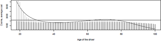
But as in Chapter 4, assuming a linear relationship might be too restrictive.
> newdb <- data.frame(AGEDRIVER=18:99,EXPOSURE=1)
> pred.poisson <- predict(reg.poisson,newdata=newdb,type="response",se=TRUE)
> plot(18:99,pred.poisson$fit,type="l",xlab="Age of the driver",
+ ylab="Annualized Frequency", ylim=c(0,.3),col="white")
> segments(18:99,pred.poisson$fit-2*pred.poisson$se.fit,
+ 18:99,pred.poisson$fit+2*pred.poisson$se.fit,col="grey",lwd=7)
> lines(18:99,pred.poisson$fit)
> abline(h=sum(CONTRACTS$NB)/sum(CONTRACTS$EXPOSURE),lty=2)
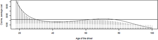
In order to get a nonparametric estimator, it is possible to consider the age (which is here an integer) as a factor variable:
> reg.np <- glm(NB~as.factor(AGEDRIVER)+offset(log(EXPOSURE)),
+ family=poisson,data=CONTRACTS)
or to use spline regressions, so that we consider a linear model including s(X) instead of X, where s() will be estimated using penalized regression splines (see Hastie & Tibshirani (1990), Bowman & Azzalini (1997), and Wood (2006) for more details):
> library(mgcv)
> reg.splines <- gam(NB~s(AGEDRIVER)+offset(log(EXPOSURE)),
+ family=poisson,data=CONTRACTS)
Predictions using the four models can be visualized in Figure 14.1 for the (standard) log- Poisson regression, and with arbitrary cuts for the age (to get a categorical variable), and in Figure 14.2 where the age is considered a factor, and using Generalized Additive Models.
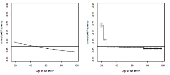
Poisson regression of the annualized frequency on the age of the driver, with a linear model, and when the age of the driver is a categorical variable.

Poisson regression of the annualized frequency on the age of the driver, per age as a factor (because it is a discrete variable) (left) and using a spline smoother (right).
14.2.6 A Poisson Regression to Model Yearly Claim Frequency
In order to have significant factors, the age of the car is here only in two classes: less than 15 years old, and more than 15 years old:
> CONTRACTS.f$AGECAR <- cut(CONTRACTS$AGECAR,c(0,15,Inf),
+ include.lowest = TRUE)
The levels are here
> levels(CONTRACTS.f$AGECAR)
[1] "[0,15]" "(15,Inf]"
For the brand, we only distinguish cars of brand F,
CONTRACTS.f$brandF <- factor(CONTRACTS.f$BRAND=="F",labels=c("other","F"))
and for the power of the car, three classes are considered here,
> CONTRACTS.f$powerF <- factor(1*(CONTRACTS.f$POWER%in%letters[4:6])+
+ 2*(CONTRACTS.f$POWER%in%letters[7:8]),
+ labels=c("other","DEF","GH"))
Our model here is
> freg <- formula(NB ~ AGEDRIVER+AGECAR+DENSITY+brandF+powerF+GAS+offset(log(EXPOSURE)))
> regp <- glm(freg,data=CONTRACTS.f,family=poisson(link="log"))
> summary(regp)
Coefficients:
Estimate Std. Error z value Pr(>|z|)
(Intercept) -1.67848 0.04652 -36.082 < 2e-16 ***
AGEDRIVER(22,26] -0.61506 0.04610 -13.341 < 2e-16 ***
AGEDRIVER(26,42] -1.08085 0.03652 -29.599 < 2e-16 ***
AGEDRIVER(42,74] -1.07777 0.03566 -30.223 < 2e-16 ***
AGEDRIVER(74,Inf] -1.10041 0.05190 -21.203 < 2e-16 ***
AGECAR(15,Inf] -0.25011 0.03085 -8.108 5.14e-16 ***
DENSITY(40,200] 0.18291 0.02676 6.834 8.26e-12 ***
DENSITY(200,500] 0.31544 0.02968 10.627 < 2e-16 ***
DENSITY(500,4.5e+03] 0.53238 0.02606 20.428 < 2e-16 ***
DENSITY(4.5e+03,Inf] 0.66731 0.03581 18.633 < 2e-16 ***
brandFF -0.18756 0.02477 -7.574 3.63e-14 ***
powerFDEF -0.17892 0.02428 -7.370 1.71e-13 ***
powerFGH -0.15361 0.02641 -5.816 6.03e-09 ***
GASRegular -0.19507 0.01620 -12.041 < 2e-16 ***
---
Signif. codes: 0 *** 0.001 ** 0.01 * 0.05 . 0.1 1
(Dispersion parameter for poisson family taken to be 1)
Null deviance: 105613 on 413168 degrees of freedom Residual deviance: 103831 on 413155 degrees of freedom AIC: 135117
Number of Fisher Scoring iterations: 6
14.3 From Poisson to Quasi-Poisson
The Poisson assumption is stronger than necessary when we use the first-order condition
?[(Yi−exp(X'iβ)).Xi]=0,
which can be rewritten as
∑ni=1(Yi−μi)g'(μi).var[Yi].Xi=0.
In this case, various forms of g(μi) (the link function) generate convergent estimatorsβ . Other forms of var[Yi] can also be chosen. In such a case, we can show that ˆβPMLE estimators have the following distributions:
ˆβPMLE→N(β,varPMLE[ˆβ]],
With
varPMLE[ˆβ]=[∑Ni=1μixix′i]−1[∑ni=1ωiXiX′i][∑ni=1μiXiX′i]−1
and ωi=var[Yi|Xi]
Obviously, if we suppose ωi=μi , we obtain the general first-order condition for a Poisson distribution:
varPMLE[ˆβ]=[∑ni=1μiXiX′i]−1=varMLE[ˆβ]
However, other forms of ωi can be explored.
14.3.1 NB1 Variance Form: Negative Binomial Type I
If we suppose an NB1 variance form, such as ωi=φμi , we have
varNB1[ˆβ]=φ[∑ni=1μixix′i]=φ.varMLE[ˆβ].
Consequently, a simple way to generalize the variance form is to use the MLE of a Poisson distribution and multiply the variance of ˆβ by an estimator ofϕ . A natural estimator of ϕ is
ˆφ=1n−k∑ni=1(yi−ˆμi)2ˆμi
but nonconstant exposition parameter Ei causes biais in the estimation. Instead, we should use
ˆφ=∑ni=1(yi−ˆμi)2∑ni=1ˆμi.
14.3.2 NB2 Variance Form: Negative Binomial Type II
If we suppose an NB2 variance form (the NB2 model is presented in detail in Section 14.4.1) such as ωi=μ+αμ2i , we have
varNB2[ˆβ]=[∑ni=1μiXiX′i]−1[∑ni=1(μi+αμ2i)XiX′i][∑ni=1μiXiX′i]−1
As with the NB1 estimator of overdispersion, the classic estimator of α is
ˆα=∑ni=1(Yi−ˆμi)2−ˆμi∑ni=1ˆμi
but is unappropriate for non-constant . The following estimator is preferred:
The NB2 regression is obtained using glm.nb of library MASS.:
> library(MASS)
> regnb2 <- glm.nb(freg,data=CONTRACTS.f)
> summary(regnb2)
Coefficients:
Estimate Std. Error z value Pr(>|z|)
(Intercept) -1.65354 0.04858 -34.037 < 2e-16 ***
AGEDRIVER(22,26] -0.63051 0.04838 -13.033 < 2e-16 ***
AGEDRIVER(26,42] -1.10163 0.03850 -28.612 < 2e-16 ***
AGEDRIVER(42,74] -1.09808 0.03765 -29.169 < 2e-16 ***
AGEDRIVER(74,Inf] -1.12431 0.05410 -20.783 < 2e-16 ***
AGECAR(15,Inf] -0.24896 0.03159 -7.882 3.23e-15 ***
DENSITY(40,200] 0.18367 0.02742 6.697 2.12e-11 ***
DENSITY(200,500] 0.31690 0.03047 10.399 < 2e-16 ***
DENSITY(500,4.5e+03] 0.53506 0.02676 19.995 < 2e-16 ***
DENSITY(4.5e+03,Inf] 0.66957 0.03690 18.148 < 2e-16 ***
brandFF -0.19253 0.02540 -7.581 3.42e-14 ***
powerFDEF -0.17756 0.02507 -7.084 1.40e-12 ***
powerFGH -0.15312 0.02726 -5.617 1.94e-08 ***
GASRegular -0.19553 0.01670 -11.707 < 2e-16 ***
---
(Dispersion parameter for Negative Binomial(0.8527) family taken to be 1)
Null deviance: 91316 on 413168 degrees of freedom Residual deviance: 89623 on 413155 degrees of freedom AIC: 134743
Number of Fisher Scoring iterations: 1
Theta: 0.8527
Std. Err.: 0.0573
2 x log-likelihood: -134712.7800
14.3.3 Unstructured Variance Form
More generally, we can estimate the variance β without supposing a specific form of . In this case, the unstructured variance form of is
evaluated at .
14.3.4 Nonparametric Variance Form
A nonparametric way to estimate is to use the approach of Delgado & Kniesner (1997). They do not suppose a specific form for the conditional variance of the i-th contract, and estimate it using a consistent estimator ofβ , , such as the one obtained by a Poisson regression:
where can be seen as weight applied to the j-th observation to compute the variance of the i-th insured with, obviously, . Using leads to an estimated variance almost equal to the empirical variance. Delgado & Kniesner (1997) evaluated the using nonparametric k nearest neighbor probabilistic weights. His method estimates variance of insured i using its k nearest neighbors, evaluated by its proximity in its normalized covariates. The k nearest neighbors were selected using a neighbor specification k that is proportional to the number of observations, such as
Instead of using the nearest neighbors estimation that gives the same weight on all k observations (which can lead to situations where the would be estimated using only insureds having the same profiles, while other would be estimated using other insured's profiles), we can rather use kernel estimation which seems to offer a better smooth.
Remark 14.2 Obviously, we can obtain a robust estimator of the variance of β by bootstrapping. By bootstrapping, we can even obtain the distribution of , instead of using the asymptotic normality of the .
14.4 More Advanced Models for Counts
A popular way to generalize count distributions is to use a compound sum of the following form:
With specific choices of distribution M and Z, we obtain the following distributions:
If , and Logarithmic , we have a negative binomial distribution.
If , and (or negative binomial), we have a Zero-inflated Poisson (or Zero-inflated negative binomial) distribution.
If , and truncated (or negative binomial), meaning that , we have a Hurdle Poisson (or Hurdle-negative binomial) distribution.
Note that instead of using a truncated at zero distribution, we can also use a shifted at zero distribution.
14.4.1 Negative Binomial Regression
In Chapters 2 and 3, it was mentioned that if , where has a Gamma distribution, with identical parameters α
(so that ), then Y has a negative binomial distribution:
which can be written
which is a distribution of the exponential family (see McCullagh & Nelder (1989)) when , with a known r. The mean of Y is here
while its variance is
which can also be written as
This is so-called Type 2 Negative Binomial regression (NB2, as in Hilbe (2011), discussed in Section 14.3.2):
The canonical link, such that
The generic function in R for an NB2 regression is
> library(MASS)
> glm.nb(Y~X1+X2+X3+offset(log(E)))
(neither the family nor the link function is specified here). In that case, is unknown and will be obtained using summary().
In the case where α is known, it is possible to use family=negative.binomiale in the standard glm function. For instance, a geometric regression will be obtained using
> glm(Y~X1+X2+X3+offset(log(E)),family=negative.binomiale(1))
In that case, .
Using the context of NB2 regression, it is possible to test if the Poisson regression is a suitable model, the alternative being an NB2 model, with α significant. We must be careful with tests when the null hypothesis is on the boundary of the parameter space. Indeed, in such situations, the MLE are no longer asymptotically normal under . The asymptotic properties of the score test, and also called the Lagrange multiplier test, as shown by Moran (1971) and Chant (1974), are not altered when testing on the boundary of the parameter space.
Using the score test, we assume here that
and we would like to test
A standard statistic is
which has a centered Gaussian distribution, with unit variance, under . This test has been implemented in R in the AER library,
> library(AER)
> dispersiontest(regp)
Overdispersion test
data: regp
z = 5.7935, p-value = 3.447e-09
alternative hypothesis: true dispersion is greater than 1
sample estimates:
dispersion
1.091931
This kind of binomial distribution (studied in Santos Silva & Windmeijer (2001)) has also been proposed with another form of parametrization. Using Equation (14.2), the parameter of the logarithmic distribution has been used as
while .
Consequently, is binomial negative with parameters and exp , with a probability function defined as
The first two moments of those models are
14.4.2 Zero-Inflated Models
A model is said to be zero-inflated if it can be written as a mixture, with probability a Dirac distribution in 0 and a standard counting regression model (Poisson or Negative Binomial):
Thus, for some counting model , for instance the Poisson distribution with parameter , then
Remark 14.3 There is a class of zero-adapted regression where
which can be used with function ZENBI of library gamlss.
If we suppose that , testing is also a test with the null hypothesis on the boundary of the parameter space. Consequently, using a score test is recommended. Van den Broek (1995) use this test and show that the test statistic of a zero-inflated Poisson against a Poisson distribution can be expressed as
Under the null hypothesis, this statistic will have an asymptotic N(0,1) distribution. Construction of the LM test for heterogeneous models against their zero-inflated modification can be done the same way.
Zero-inflated and zero-adapted models can be estimated either using functions ZIP (zero- inflated Poisson) or ZAP (zero-adapted Poisson), or functions ZINI (zero-inflated Negative Binomial) or ZIBI (zero-adapted Negative Binomial) from library gamlss, or functions of library pscl (described in Zeileis et al. (2008)). For instance, for a zero-inflated model, where probability is function of covariates (with a logistic transformation), while , is function of covariates , the generic code will be
> reg <- zeroinfl(NB ~ X1 | X2 , data=CONTRACTS.f , dist = "poisson" ,
+ link="logit"))
If we consider a zero-inflated Poisson model, with constant probability , we obtain
> fregzi <- formula(NB ~ AGEDRIVER+AGECAR+DENSITY+brandF+powerF+
+ GAS+offset(log(EXPOSURE))|1)
> regzip=zeroinfl(fregzi,data=CONTRACTS.f,dist = "poisson",link="logit")
> summary(regzip)
Pearson residuals:
Min 1Q Median 3Q Max
-0.4907 -0.2315 -0.1827 -0.1038 101.3696
Count model coefficients (poisson with log link):
Estimate Std. Error z value Pr(>|z|)
(Intercept) -0.92717 0.05953 -15.574 < 2e-16 ***
AGEDRIVER(22,26] -0.62772 0.04872 -12.885 < 2e-16 ***
AGEDRIVER(26,42] -1.09943 0.03885 -28.302 < 2e-16 ***
AGEDRIVER(42,74] -1.09585 0.03799 -28.844 < 2e-16 ***
AGEDRIVER(74,Inf] -1.11988 0.05431 -20.619 < 2e-16 ***
AGECAR(15,Inf] -0.24825 0.03167 -7.839 4.54e-15 ***
DENSITY(40,200] 0.18379 0.02746 6.693 2.18e-11 ***
DENSITY(200,500] 0.31679 0.03051 10.382 < 2e-16 ***
DENSITY(500,4.5e+03] 0.53457 0.02679 19.951 < 2e-16 ***
DENSITY(4.5e+03,Inf] 0.67016 0.03692 18.150 < 2e-16 ***
brandFF -0.19000 0.02539 -7.483 7.25e-14 ***
powerFDEF -0.17657 0.02507 -7.042 1.90e-12 ***
powerFGH -0.15223 0.02727 -5.583 2.37e-08 ***
GASRegular -0.19499 0.01672 -11.660 < 2e-16 ***
Zero-inflation model coefficients (binomial with logit link):
Estimate Std. Error z value Pr(>|z|)
(Intercept) 0.07414 0.06441 1.151 0.25
---
Signif. codes: 0 '***' 0.001 '**' 0.01 '*' 0.05 '.' 0.1 ' ' 1
Number of iterations in BFGS optimization: 25
Log-likelihood: -6.736e+04 on 15 Df
Number of iterations in BFGS optimization: 25 Log-likelihood: -6.736e+04 on 15 Df
If we consider a probability function of the age of the driver, we obtain
> fregzi <- formula(NB ~ AGEDRIVER+AGECAR+DENSITY+brandF+powerF+
+ GAS+offset(log(EXPOSURE))|AGEDRIVER)
> regzip=zeroinfl(fregzi,data=CONTRACTS.f,dist = "poisson",link="logit")
> summary(regzip)
Pearson residuals:
Min 1Q Median 3Q Max
-0.4946 -0.2306 -0.1827 -0.1038 101.3908
Count model coefficients (poisson with log link):
Estimate Std. Error z value Pr(>|z|)
(Intercept) -0.96211 0.11575 -8.312 < 2e-16 ***
AGEDRIVER(22,26] -0.39498 0.15828 -2.496 0.0126 *
AGEDRIVER(26,42] -1.09883 0.12822 -8.570 < 2e-16 ***
AGEDRIVER(42,74] -1.10280 0.12236 -9.013 < 2e-16 ***
AGEDRIVER(74,Inf] -0.74634 0.18353 -4.067 4.77e-05 ***
AGECAR(15,Inf] -0.24745 0.03167 -7.813 5.57e-15 ***
DENSITY(40,200] 0.18414 0.02746 6.706 1.99e-11 ***
DENSITY(200,500] 0.31706 0.03051 10.391 < 2e-16 ***
DENSITY(500,4.5e+03] 0.53491 0.02679 19.964 < 2e-16 ***
DENSITY(4.5e+03,Inf] 0.67015 0.03691 18.154 < 2e-16 ***
brandFF -0.18993 0.02538 -7.483 7.27e-14 ***
powerFDEF -0.17644 0.02506 -7.041 1.91e-12 ***
powerFGH -0.15233 0.02725 -5.591 2.26e-08 ***
GASRegular -0.19486 0.01672-11.655 < 2e-16 ***
Zero-inflation model coefficients (binomial with logit link):
Estimate Std. Error z value Pr(>|z|)
(Intercept) 0.0083752 0.2036001 0.041 0.9672
AGEDRIVER(22,26] 0.4143760 0.2695767 1.537 0.1243
AGEDRIVER(26,42] -0.0003184 0.2382535 -0.001 0.9989
AGEDRIVER(42,74] -0.0152864 0.2267851 -0.067 0.9463
AGEDRIVER(74,Inf] 0.6404166 0.2952266 2.169 0.0301 *
---
Signif. codes: 0 '***' 0.001 '**' 0.01 '*' 0.05 '.' 0.1 ' ' 1
Number of iterations in BFGS optimization: 61
Log-likelihood: -6.736e+04 on 19 Df
14.4.3 Hurdle Models
The Hurdle distribution is based on a dichotomic process, where insureds that report are considered completely different from those who report at least once. For some specific probability mass functions and , the probability function of the hurdle is expressed as
The model collapses to when , which can be used as a basis for a specification test. The mean and variance corresponding to the model described above are given by
where is the expected value associated with the probability mass function .
An advantage of the model is its property to have a separable log-likelihood:
Then, as done with the number of claims and the cost of the claims, the maximization of the log-likelihood can be done separately for each part (zero case and positive values).
These models can be implemented using the hurdle function, from the pscl library. If we consider a (truncated) negative binomial distribution for and a binomial distribution for , on covariates respectively, the generic code will be
> hurdle(NB ~ X1 | X2 , data=CONTRACTS.f, dist = "poisson",
+ zero.dist = "binomial")
Here, we obtain
> freghrd <- formula(NB ~ AGEDRIVER+AGECAR+DENSITY+brandF+powerF+
+ GAS+offset(log(EXPOSURE))|AGEDRIVER)
> reghrd=hurdle(freghrd,data=CONTRACTS.f,dist = "negbin",zero.
+ dist = "binomial", link = "logit")
> summary(reghrd)
Pearson residuals:
Min 1Q Median 3Q Max
-0.2787 -0.1959 -0.1924 -0.1825 21.7379
Count model coefficients (truncated negbin with log link):
Estimate Std. Error z value Pr(>|z|)
(Intercept) -2.92542 0.94540 -3.094 0.001972 **
AGEDRIVER(22,26] -0.37124 0.18182 -2.042 0.041171 *
AGEDRIVER(26,42] -1.10622 0.14957 -7.396 1.40e-13 ***
AGEDRIVER(42,74] -1.12550 0.14375 -7.829 4.90e-15 ***
AGEDRIVER(74,Inf] -0.72592 0.20704 -3.506 0.000455 ***
AGECAR(15,Inf] -0.02225 0.16247 -0.137 0.891071
DENSITY(40,200] 0.45729 0.15381 2.973 0.002949 **
DENSITY(200,500] 0.41196 0.16760 2.458 0.013973 *
DENSITY(500,4.5e+03] 0.69487 0.14832 4.685 2.80e-06 ***
DENSITY(4.5e+03,Inf] 1.14389 0.17446 6.557 5.50e-11 ***
brandFF 0.80303 0.10326 7.777 7.43e-15 ***
powerFDEF 0.19143 0.11868 1.613 0.106739
powerFGH 0.06720 0.12951 0.519 0.603820
GASRegular -0.10676 0.07777 -1.373 0.169835
Log(theta) -0.87532 1.33388 -0.656 0.511683
Zero hurdle model coefficients (binomial with logit link):
Estimate Std. Error z value Pr(>|z|)
(Intercept) -2.55504 0.03645 -70.09 <2e-16 ***
AGEDRIVER(22,26] -0.50876 0.04940 -10.30 <2e-16 ***
AGEDRIVER(26,42] -0.82424 0.03908 -21.09 <2e-16 ***
AGEDRIVER(42,74] -0.68664 0.03823 -17.96 <2e-16 ***
AGEDRIVER(74,Inf] -0.59923 0.05535 -10.83 <2e-16 ***
---
Signif. codes: 0 '***' 0.001 '**' 0.01 '*' 0.05 '.' 0.1 ' ' 1
Theta: count = 0.4167
Number of iterations in BFGS optimization: 57
Log-likelihood: -6.869e+04 on 20 Df
14.5 Individual Claims, Gamma, Log-Normal, and Other Regressions
In the introduction, we have seen that the pure premium associated to an insured with characteristics x should be . The first part has been detailed in the previous sections, and now it might be time to propose some models for individual claims losses . This section is usually described briefly in actuarial literature, because the tools used are the same as before (Generalized Linear Models); so for statistical reasons, there is no reason to spend too much time here. But also because, in practice, covariates are much less informative to predict amounts than to predict frequency. The dataset contains a claims ID (which is a contract number) and an indemnity amount:
> tail(CLAIMS)
ID INDEMNITY
16176 303133 769
16177 302759 61
16178 299443 1831
16179 303389 4183
16180 304313 566
16181 206241 2156
It is possible to merge this dataset with the one that contains information about the contracts:
claims <- merge(CLAIMS,CONTRACTS)
claims.f <- merge(CLAIMS,CONTRACTS.f)
Note that this dataset contains only claims with a strictly positive indemnity (losses claims but filed away are not in this dataset). Thus, what we need to model losses is a distribution on R+.
14.5.1 Gamma Regression
Y has a Gamma distribution if its density can be written
This distribution is in the exponential family, as
The canonical link here is , so that the variance function will be . Observe, further, that var , and thus the coefficient of variation is constant; here,
Remark 14.4 A particular distribution in this family is the exponential distribution, with density
and mean .
14.5.2 The Log-Normal Model
Y has a log-normal distribution if its density can be written
which is not in the exponential family (so Generalized Linear Models cannot be used to model Y). Nevertheless, recall that Y has a log-normal distribution if log Y has a Gaussian distribution (which is in the exponential family).
Remark 14.5 f Y has a log-normal distribution with parameters and , then Thus, is not the average of Y, and neither is . In fact,
, from Jensen inequality. One can easily prove that
14.5.3 Gamma versus Log-Normal Models
Consider a Gamma regression for . Using Taylor's expansion (of order 2),
if φ is small. Then, if we take the expected value, it comes that
Further, one can also prove that var . If we consider a logarithm link function, so that has variance then
Consider now a log-normal regression, i.i.d. Then
Except for the intercept, coefficients α and β should be rather close if the coefficient of variation is small
> reg.logn <- lm(log(INDEMNITY)~AGECAR+GAS,
+ data=claims[claims$INDEMNITY<15000,])
> reg.gamma <- glm(INDEMNITY~AGECAR+GAS,family=Gamma(link="log"),
+ data=claims[claims$INDEMNITY<15000,])
> summary(reg.gamma)
Coefficients:
Estimate Std. Error t value Pr(>|t|)
(Intercept) 7.26172 0.02568 282.772 < 2e-16 ***
AGECAR(1,4] 0.02127 0.03095 0.687 0.49194
AGECAR(4,15] -0.07575 0.02713 -2.792 0.00525 **
AGECAR(15,Inf] -0.08397 0.04048 -2.074 0.03807 *
GASRegular -0.02307 0.01719 -1.342 0.17950
Signif. codes: 0 *** 0.001 ** 0.01 * 0.05 . 0.1 1
(Dispersion parameter for Gamma family taken to be 1.166754)
Null deviance: 13410 on 16002 degrees of freedom
Residual deviance: 13377 on 15998 degrees of freedom
AIC: 261934
Number of Fisher Scoring iterations: 5
> summary(reg.logn)
Coefficients:
Estimate Std. Error t value Pr(>|t|)
(Intercept) 6.8475524 0.0247901 276.221 < 2e-16 ***
AGECAR(1,4] 0.0004851 0.0298728 0.016 0.98704
AGECAR(4,15] -0.0803790 0.0261929 -3.069 0.00215 **
AGECAR(15,Inf] -0.0306088 0.0390797 -0.783 0.43350
GASRegular -0.0240781 0.0165916 -1.451 0.14674
---
Signif. codes: 0 *** 0.001 ** 0.01 * 0.05 . 0.1 1
Residual standard error: 1.043 on 15998 degrees of freedom
Multiple R-squared: 0.001459, Adjusted R-squared: 0.00121
F-statistic: 5.845 on 4 and 15998 DF, p-value: 0.000107
Remark 14.6 One can prove that for a Gamma regression, the inverse of Fisher information for (which will be the asymptotic variance) is , which is exactly the variance of in the log-normal model.
14.5.4 Inverse Gaussian Model
Y has an inverse Gaussian distribution if its density can be written
with expected value .
14.6 Large Claims and Ratemaking
If claims are not too large, then the log-normal and the gamma regressions should be quite close, as mentioned in the section above. But consider the following two regressions, on the age of the driver (as a continuous variate):
> reg.logn <- lm(log(INDEMNITY)~AGEDRIVER,data=claims)
> reg.gamma <- glm(INDEMNITY~AGEDRIVER,family=Gamma(link="log"),data=claims)
> summary(reg.gamma)
Coefficients:
Estimate Std. Error t value Pr(>|t|)
(Intercept) 8.095074 0.203485 39.782 <2e-16 ***
AGEDRIVER -0.009926 0.004304 -2.307 0.0211 *
---
Signif. codes: 0 *** 0.001 ** 0.01 * 0.05 . 0.1 1
(Dispersion parameter for Gamma family taken to be 66.85011)
> summary(reg.logn)
Coefficients:
Estimate Std. Error t value Pr(>|t|)
(Intercept) 6.7361807 0.0277458 242.782 < 2e-16 ***
AGEDRIVER 0.0020374 0.0005868 3.472 0.000518 ***
Signif. codes: 0 *** 0.001 ** 0.01 * 0.05 . 0.1 1
Residual standard error: 1.115 on 16179 degrees of freedom
Here, coefficients are significant, but with opposite signs. With a Gamma regression, the younger the driver, the less expensive the claims, while it is the reverse with a log-normal regression. The interpretation is related to large claims: outliers will affect the Gamma regression more than the log-normal one (because it is a regression on the logarithm of losses). On the other hand, on average, predictions obtained with a log-normal model may not be consistent with observed losses: here, the average cost of the claim was
> mean(claims$INDEMNITY)
[1] 2129.972
and the average predictions were, with the two models,
> mean(predict(reg.gamma,type="response"))
[1] 2130.361
> sigma <- summary(reg.logn)$sigma
> mean(exp(predict(reg.logn))*exp(sigma"2/2))
[1] 1718.981
So, in order to have a more robust pricing method, we should find a way to deal with large claims (see also Teugels (1982) for a discussion of the concept of large claims, or Beirlant & Teugels (1992)). A natural technique is to consider that differentiating premiums should be valid for standard claims, while extremely large ones might be spread between all the insureds, without differentiating (pooling extremely large losses among the insureds).
> M <- claims[order(-claims$INDEMNITY),c("INDEMNITY","NB","POWER",
+ "AGECAR","AGEDRIVER","GAS","DENSITY")]
> M$SUM <- cumsum(M$INDEMNITY)/sum(M$INDEMNITY)*100
> head(M)
INDEMNITY NB POWER AGECAR AGEDRIVER GAS DENSITY SUM
5033 2036833 1 i 13 19 Regular 93 5.909
1854 1402330 2 f 13 20 Regular 203 9.978
4948 306559 1 g 1 21 Diesel 108 10.868
2637 301302 1 f 3 46 Diesel 10 11.742
11566 281403 1 f 4 61 Diesel 1064 12.558
4512 254944 1 d 12 27 Regular 319 13.298
The largest claim cost more than 2 million euros, almost 6% of the total loss. The three largest (almost 11% of the total loss) were caused by young drivers (19, 20, and 21 years old, respectively).
14.6.1 Model with Two Kinds of Claims
A standard result in probability theory is that for any Z. Thus, given a multinomial random variable Z, taking values 's,
on any probabilistic space. Thus, we can consider any conditional expectation
.
Consider the case where Z is some information about the size of the claim, namely Z belongs either to , for some high amount s. Therefore,
As before, in the case where the probability is computed under conditional probability, given X, the relationship above becomes
where
- A is the average cost of normal claims (excluding claims that exceed s)
- B is the average cost of large claims (those that exceed s)
- C is the probability of having a large or a normal claim
For part C, a logistic regression can be run. For parts A and B, regressions are on subsets of the dataset. Consider a threshold s <- 10000, reached by less than 2% of the claims:
> claims$STANDARD <- (claims$INDEMNITY<s)
> mean(claims$STANDARD)
[1] 0.982943
Consider a logistic regression to model the probability that a claim will be a standard one:
> library(splines)
> age <- seq(18,100)
> regC <- glm(STANDARD~bs(AGEDRIVER),data=claims,family=binomial)
> ypC <- predict(regC,newdata=data.frame(AGEDRIVER=age),type="response",
se=TRUE)
The probability can be visualized in Figure 14.3:
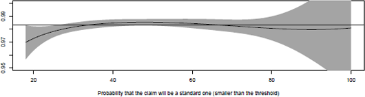
Probability of having a standard claim, given that a claim occurred, as a function of the age of the driver. Logistic regression with a spline smoother.
plot(age,ypC$fit,ylim=c(.95,1),type="l",)
polygon(c(age,rev(age)),c(ypC$fit+2*ypC$se.fit,rev(ypC$fit-2*ypC$se.fit)), + col="grey",border=NA)
abline(h=mean(claims$STANDARD),lty=2)
For standard and large claims, consider two gamma regressions on the two subsets,
indexstandard <- which(claims$INDEMNITY<s)
mean(claims$INDEMNITY[indexstandard])
[1] 1280.085
mean(claims$INDEMNITY[-indexstandard])
[1] 51106.23
regA <- glm(INDEMNITY~bs(AGEDRIVER),data=claims[indexstandard,],
+ family=Gamma(link="log"))
ypA <- predict(regA,newdata=data.frame(AGEDRIVER=age),type="response")
regB <- glm(INDEMNITY~bs(AGEDRIVER),data=claims[-indexstandard,],
+ family=Gamma(link="log"))
ypB <- predict(regB,newdata=data.frame(AGEDRIVER=age),type="response")
In order to compare, let us fit one model on the overall dataset:
reg <- glm(INDEMNITY~bs(AGEDRIVER),data=claims,family=Gamma(link="log"))
yp <- predict(reg,newdata=data.frame(AGEDRIVER=age),type="response")
and let us compare the two approaches, on Figure
ef{Fig:GLM:age-small-large}
ypC <- predict(regC,newdata=data.frame(AGEDRIVER=age),type="response")
plot(age,yp,type="l",lwd=2,ylab="Average cost",xlab="Age of the driver")
lines(age,ypC*ypA+(1-ypC)*ypB,type="h",col="grey",lwd=6)
lines(age,ypC*ypA,type="h",col="black",lwd=6)
abline(h= mean(claims$INDEMNITY),lty=2)
The dotted horizontal line in Figure 14.3 is the average cost of a claim. The dark line, in the back, is the prediction on the whole dataset reg. The dark part is the part of the average claim related to standard claims (smaller than s) and the lighter area is the part of the average claim due to possible large claims (exceeding s).
For standard and large claims, consider two gamma regressions, on the two subsets. As mentioned earlier, it is possible to substitute constant parts in the pricing model, for example,
where is obtained by considering the average cost of large claims, without any explanatory variable.
It is possible to focus not on large claims, but on extremely large claims, s <- 100000, as on Figure 14.6, where three smoothed regressions are considered.
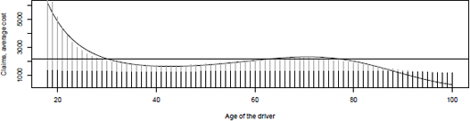
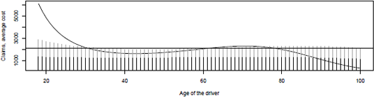
Average cost of a claim, as a function of the age of the driver, s =10,000, when extremely large claims are pooled among the insured.
14.6.2 More General Model
A more general model can be considered here:
where mixing probabilities are associated to a multinomial random variable.
A multinomial regression model can be written, as an extension of the logistic regression one. Assume here that
The estimation of coefficients and (including standard errors) can be obtained using regression multinom of library(nnet) :
> library(nnet)
> threshold <- c(0,1150,10000,Inf)
> regD <- multinom(cut(claims$INDEMNITY,breaks=threshold)~bs(AGEDRIVER),data=claims) # weights: 15 (8 variable)
initial value 17776.645443 iter 10 value 12391.379124 final value 12389.058985 converged
> summary(regD)
Call:
multinom(formula = cut(claims$INDEMNITY, breaks = threshold) ~ bs(AGEDRIVER), data = claims)
Coefficients:
(Intercept) bs(AGEDRIVER)1 bs(AGEDRIVER)2 bs(AGEDRIVER)3
(1.15e+03,1e+04] 0.126849 -0.5866635 0.4435400 0.2998493
(1e+04,Inf] -2.716344 -1.8494277 0.1237384 -0.2909207
Std. Errors:
(Intercept) bs(AGEDRIVER)1 bs(AGEDRIVER)2 bs(AGEDRIVER)3
(1.15e+03,1e+04] 0.06893703 0.2353106 0.2562023 0.3562258
(1e+04,Inf] 0.22592318 0.8219250 0.9575998 1.2674017
Residual Deviance: 24778.12
AIC: 24794.12
For instance, for drivers with age 20 or 50, given that a claim has occurred, the probability that it could be in one of the three tranches will be
> predict(regD,newdata=data.frame(AGEDRIVER=c(20,50)),type="probs")
(0,1.15e+03] (1.15e+03,1e+04] (1e+04,Inf]
1 0.4655077 0.5074693 0.02702298
2 0.4885641 0.4967026 0.01473323
If we plot the parts due to small claims (less than ), medium claims (from to ), and large claims (more than ), we obtain the graph in Figure 14.7
Probability of having a standard claim, given that a claim occurred, as a function of the age of the driver. Logistic regression with a spline smoother.
14.7 Modeling Compound Sum with Tweedie Regression
As a conclusion, we can mention a large class of Generalized Linear Models, called Tweedie models in Jprgensen (1987), studied in Jprgensen (1997). A Tweedie distribution is in the exponential family, and it satisfies
If is the distribution with constant variance (normal distribution), if , then the variance function is linear (Poisson distribution); and if , it has a quadratic variance function (Gamma distribution).
An interesting case is when p lies in the interval (1, 2). In that case, Y is a compound Poisson-Gamma distribution. A natural idea is then to use a Tweedie model on the aggregated sum, per insured.
> A <- tapply(CLAIMS$INDEMNITY,CLAIMS$ID,sum)
> ADF <- data.frame(ID=names(A),INDEMNITY=as.vector(A))
> CT <- merge(CONTRACTS,ADF,all.x = TRUE)
> CT$INDEMNITY[is.na(CT$INDEMNITY)] <- 0
> tail(CT)
NB EXPOS POWER AGECAR AGEDRIVER BRAND GAS REGION DENSITY IND
413164 0 0.005 d 0 61 F Regular 25 205 0
413165 0 0.002 j 0 29 F Diesel 11 2471 0
413166 0 0.005 d 0 29 F Regular 11 5360 0
413167 0 0.005 k 0 49 F Diesel 11 5360 0
413168 0 0.002 d 0 41 F Regular 11 9850 0
413169 0 0.002 g 6 29 F Diesel 72 65 0
> CT.f=merge(CONTRACTS.f,ADF,all.x = TRUE)
> CT.f$INDEMNITY[is.na(CT.f$INDEMNITY)] <- 0
> tail(CT.f)
NB EXPOS POWER AGECAR AGEDRIVER BRAND GAS REGION DENSITY IND
413164 0 0.005 d [0,1] (42,74] F Regular 25 (200,500] 0
413165 0 0.002 j [0,1] (26,42] F Diesel 11 (500,4.5e+03] 0
413166 0 0.005 d [0,1] (26,42] F Regular 11 (4.5e+03,Inf] 0
413167 0 0.005 k [0,1] (42,74] F Diesel 11 (4.5e+03,Inf] 0
413168 0 0.002 d [0,1] (26,42] F Regular 11 (4.5e+03,Inf] 0
413169 0 0.002 g (4,15] (26,42] F Diesel 72 (40,200] 0
Using library tweedie we obtain
> out <- tweedie.profile(INDEMNITY~POWER+AGECAR+
+ AGEDRIVER+BRAND+GAS+DENSITY,data=CT.f,
+ p.vec=seq(1.05,1.95,by=.05))
We can then plot the profile likelihood function associated to the Tweedie regression:
> out$p.max [1] 1.564286
> plot(out,type="b")
> abline(v=out$p.max,lty=2)
In order to ensure convergence of the algorithm, we can use coefficients obtained from a Poisson regression:
reg1 <- glm(INDEMNITY~POWER+AGECAR+AGEDRIVER+BRAND+GAS+DENSITY,
+ data=CT.f, family = tweedie(var.power = 1, link.power =0))
The following function returns as a function of p:
> coef <- function(p){
+ glm(INDEMNITY~POWER+AGECAR+AGEDRIVER+BRAND+GAS+DENSITY,
+ data=CT.f, family = tweedie(var.power = p, link.power = 0),
+ start=reg1$coefficients)$coefficients}
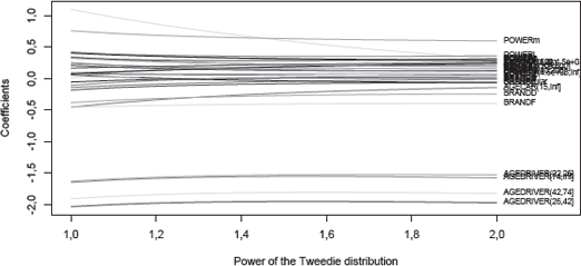
It is also possible to visualize the evolution of the coefficients estimates as a function of p (without the (Intercept)), with a logarithm link function:
> vp <- seq(1,2,by=.1)
> Cp <- Vectorize(coef)(vp)
> matplot(vp,t(Cp[-1,]),type="l")
> text(2,Cp[-1,length(vp)],rownames(Cp[-1,]),cex=.5,pos=4)

One can also use library cplm for fitting Tweedie compound Poisson linear models. Smyth & Jprgensen (2002) suggested a Tweedie model using a joint likelihood function (for claim cost and frequency).
14.8 Exercises
- 14.1. In the minimum bias method, based on the least squares approach we have to minimize
- Write the first-order condition, and solve this equation, numerically, on the same variables as in Section 14.2.4.
- 14.2. In the minimum bias method, based on the chi-square approach, we have to minimize
- Write the first-order condition, and solve this equation, numerically, on the same variables as in Section 14.2.4.