Chapter 3

Bayesian Philosophy

Benedict Escoto

AON Benfield
Chicago, Illinois, United States

Arthur Charpentier

Universite du Quebec a Montreal
Montreal, Quebec, Canada

3.1 Introduction

Bayesian philosophy has a long history in actuarial science, even if it was sometimes hidden. Liu et al. (1996) claim that “Statistical methods with a Bayesian flavor [...] have long been used in the insurance industry.” And according to McGrayne (2012), actuaries and Arthur L. Bailey played an important rule to prove that it might be relevant to have prior opinions about the next experiment, not to say credible.

“[Arthur] Bailey spent his first year in New York [in 1918] trying to prove to himself that 'all of the fancy actuarial [Bayesian] procedures of the casualty business were mathematically unsound.' After a year of intense mental struggle, however, he realized to his consternation that actuarial sledgehammering worked. He even pre­ferred it to the elegance of frequentism. He positively liked formulae that described 'actual data ... I realized that the hard-shelled underwriters were recognizing cer­tain facts of life neglected by the statistical theorists.' He wanted to give more weight to a large volume of data than to the frequentists small sample; doing so felt surprisingly 'logical and reasonable.' He concluded that only a 'suicidal' actuary would use Fisher's method of maximum likelihood, which assigned a zero probabil­ity to nonevents. Since many businesses file no insurance claims at all, Fisher's method would produce premiums too low to cover future losses.”

3.1.1 A Formal Introduction

Lindley (1983) explained the Bayesian paradigm as follows. The interest here is a quantity θ, which is unknown. But we might have some personal idea about its distribution that should express our relative opinion as to the likelihood that various possible values of θ are the true value. This will be the prior distribution of θ, and it will be denoted π(θ). This represents the state of our knowledge, somehow, prior to conducting an experiment, or observing the data. Further, there is a probability distribution f (x|θ), which describes the relative likelihood of values x, given that θ is the true parameter value, for a random variable X. But there is nothing new here. As discussed in Chapter 2, this is the parametric distribution of a random variable X, that was sometimes denoted $f_{\theta }\left(x\right)$. The main difference might be that θ is a random variable here, and thus $f_{\theta }\left(x\right)$ is now a conditional distribution, of X, given the information that θ is the true value.

Based on those two functions, we use Bayes theorem to compute

${\pi }^{\ast }\left(\theta |x\right)=\frac{f\left(x|\theta \right)\pi \left(\theta \right)}{\int f\left(x|\theta \right)\pi \left(\theta \right)d\theta },$

which is the posterior distribution of θ. It can be seen as a revised opinion, once the results of the experiment are known. Once we have this posterior distribution, which contains all the knowledge we have (our subjective a priori, and the sample, which can be seen as more objective), we can compute any quantity of interest. This can be done either using analytical formulas, when the later are tractable, or using Monte Carlo simulations to generate possible values θ , given the sample that was observed.

Consider, for instance, the case where θ is a position measure that can be the mode, the median, the mean, etc. In the classical and standard setting (see Chapter 2), we usually compute confidence intervals, so that we can claim that with probability 1 —α, θ belongs to some interval. In the Bayesian framework, we compute a 1 —α credibility interval, so that

$\text{ℙ}\left(\theta \in \left[\ell ,u\right]|X\right)=\underset{\ell }{\overset{u}{\int }}{\pi }^{\ast }\left(\theta |X\right)d\theta =1-\alpha$

We can also use a Bayesian version of the Central Limit Theorem (see Berger (1985)) to derive a credibility interval: Under suitable conditions, the posterior distribution can be approximated with a Gaussian distribution, and an approximated credibility interval is then

$?\left(\theta |X\right)\pm {\Phi }^{-1}\left(1-\alpha /2\right)\sqrt{\text{Var}\left(\theta |X\right)}.$

3.1.2 Two Kinds of Probability

There are two kinds of probability: objective and subjective. Roughly speaking, objective probabilities are defined by reality via scientific laws and physical processes. Subjective probabilities are created by people to help them quantify their beliefs and analyze the consequences of their beliefs.

For example, take the sentences in Table 3.1. The sentences in the first row are objective. Whether or not the coin is fair (50% probability of heads) or biased depends not on what anyone believes about the coin, but on the physical properties of the coin (its shape and distribution of mass).

On the other hand, the sentences in the second row seem less objective. Life exists on other planets or not; it is not clear what would make it objectively true that the probability of this is 90%. A probability like this varies across people and reflects strength of belief.

Although the exact boundary between subjective and objective probability is contro­versial, the basic distinction itself is somewhat obvious. It is important to this chapter because this distinction is what distinguishes Bayesian from classical statistics. Bayesians find it useful to deal with subjective probabilities. On the other hand, classical statisticians think only objective probabilities are worthwhile, either because subjective probabilities are nonsensical or because they are too subjective.

3.1.3 Working with Subjective Probabilities in Real Life

How would subjective probabilities that are just about beliefs have any practical value? Consider the following argument:

1. There is a 50% chance that liability costs per exposure will decrease.
2. Independent of liability costs, there is a 50% chance that our CEO will decide to reduce expenses.
3. Our company will only be profitable if and only if liability costs decrease and the CEO reduces expenses.
4. Therefore, there is less than a 25% chance we will make a profit.

Although statements (1) and (2) may be purely subjective probabilities, an argument like the one above can still be powerful. Even though the first two statements may not be objectively true or false, someone who endorses (1)-(3) and yet rejects (4) seems to be in error.

Bayesian statistics really gets going when you add the principle of conditionalization:

If your beliefs are associated with probability function P, and you learn evidence e, then your new beliefs should now be associated with probability function ${\mathbb{P}}_e$, where for all x,

${\mathbb{P}}_e\left(x\right)=\mathbb{P}\left(x|e\right).$ Either by definition or axiom, $\mathbb{P}\left(x|e\right)=\frac{\mathbb{P}\left(x\wedge e\right)}{\mathbb{P}\left(e\right)}.$

We call P(x) the prior probability of x because it is the probability of x prior to learning the evidence e. Similarly, ${\mathbb{P}}_e\left(x\right)=\mathbb{P}\left(x|e\right).$ is called the posterior probability of x.

With the principle of conditionalization, Bayesian statistics provides a simple yet pow­erful suggestion about belief dynamics: how a person's beliefs should change when he or she learns new things. For instance, suppose we add to the sentences (1)-(4) above:

1. The CEO has decided to reduce expenses.
2. The new probability that we will make a profit is 50%.

When (5) is learned, then (6) describes the new probablitiy of a profit via the conditional- ization rule.

3.1.4 Bayesianism for Actuaries

More than a hundred years ago, actuaries observed that when setting insurance premiums, the best ratemaking was obtained when the premium was somewhere between the actual experience of the insured and the overall average for all insureds. The mathematical for­mulation yields to the credibility theory, which has strong connections with the Bayesian philosophy.

Bayesianism seems a natural fit for actuaries. As claimed in Klugman (1992), “within the realm of actuarial science there are a number of problems that are particularly suited for Bayesian analysis.” Actuaries are known for their numerical literacy, so it may be natural for them to quantify the strength of their beliefs via probabilities. Actuaries are valued for their extensive industry knowledge judgment, so their considered beliefs make useful starting points in statistical analyses.

On the other hand, actuaries also prize objectivity. They like to communicate facts and unimpeachable analyses to their employers and clients, and are not content merely because their beliefs are probabilistically consistent. The rest of this chapter will introduce several applications of Bayesian reasoning. The chapter's conclusion will revisit the pros and cons of Bayesianism for actuaries.

3.2 Bayesian Conjugates

As we will see shortly, although Bayesianism has a simple statement, its implementation often requires complex computations. However, this complexity can often be sidestepped using Bayesian conjugates, also called conjugate distributions.

3.2.1 Historical Perspective

Pierre-Simon Laplace observed, from 1745 to 1784, 770,941 births: 393,386 boys and 377,555 girls. Assuming the sex of a baby is a Bernoulli random variable, so that p denotes the probability of having a boy, Pierre-Simon Laplace wanted to quantify the credibility of the hypothesis $p\ge 0.5$. His idea was to assume that a priori, p might be uniformly distributed on the unit interval, and then, given statistics observed, to compute the a posteriori probability that $p\ge 0.5$. If N is the number of boys, out of n0 births, then

$f\left(p|N=n\right)=\frac{\pi \left(p\right)\cdot \mathbb{P}\left(N=n|p\right)}{\mathbb{P}\left(N=n\right)}\propto \left(\begin{array}{c}n\\ n_0\end{array}\right)p^n{\left(1-p\right)}^{n_o-n}$

Observe that

$f\left(p|N=n\right)\propto \underset{\text{prior}}{\underbrace{\pi \left(p\right)}}\cdot \underset{\text{likelihood}}{\underbrace{\mathbb{P}\left(N=n|p\right)}},$

as mentioned in the introduction. A more general model is to assume that a priori p has a beta distribution, $p\sim B\left(\alpha ,\beta \right)$. Then

$f\left(p|N=n\right)\propto p^{\alpha +n}{\left(1-p\right)}^{\beta +n_0-n}$

which is the density of a beta distribution, $B\left(\alpha +n,\beta +n_0-n\right)$. As a consequence,

$\text{?}\left(p|N=n\right)=\frac{\alpha +n}{\alpha +\beta +n_0}\approx \frac{n}{n_0}$

when n is large enough, and

$\mathrm{var}\left(p|N=n\right)=\frac{\left(\alpha +n\right)\left(\beta +n_0-n\right)}{{\left[\alpha +\beta +n_0\right]}^2\left(\alpha +\beta +n+1\right)}\approx \frac{n\left(n_0-n\right)}{n\begin{array}{c}3\\ 0\end{array}}=\frac{1}{n_0}\cdot \frac{n}{n_0}\left(1-\frac{n}{n_0}\right)\cdot$

In this example, the distribution of the variable of interest is in the exponential family (here a binomial distribution), and the a priori distribution is the conjugate distribution (here a beta distribution).

Consider another example, where after discussing with 81 agents, 51 answered positively to some proposition. We would like to test whether this proposition exceeds 2/3, or not. Let $X=\left(X_1,\mathrm{....},X_n\right)$ denote the answers of the n agents, $X_i$ is 1 when they answered positively, otherwise 0. Here, $X_i\sim B\left(\theta \right)$, and the Bayesian interpretation of the test is based on the computation of $\mathbb{P}\left(\theta >2/3|X\right)$. Consider a priori beta distribution for θ, so that $\theta \sim B\left(\alpha ,\beta \right)$. Then

$\theta |X=x\sim B\left(\alpha +\sum x_i,\beta +n-\sum x_i\right)$

To visualize the prior and the posterior distribution, consider the following code:

> n <- 81

> sumyes <- 51

> priorposterior <- function(a,b){

+ u <- seq(0,1,length=251)

+ prior <- dbeta(u,a,b)

+ posterior <- dbeta(u,sumyes+a,n-sumyes+b)

+ plot(u,posterior,type="l",lwd=2)

+ lines(u,prior,lty=2)

+ abline(v=(sumyes+a)/(n+a+b),col="grey")}

Assuming a flat prior, $\pi \left(\theta \right)\propto 1,$ corresponds to a uniform distribution, obtained when $\alpha =\beta =1$.

> priorposterior(1,1)

An alternative can be to consider a more informative prior, for instance, $\alpha =5\text{ and }\beta =3:$

> priorposterior(5,3)

Those distributions can be visualized on Figure 3.1, the dotted line being the prior distri­bution, and the solid one the posterior. The vertical straight line represents the posterior mean.

If we get back to the initial question, $\mathbb{P}\left(\theta >2/3|X\right)$ can be obtained easily as

> 1-pbeta(2/3,1+51,1+81-51)

[1] 0.2273979

> 1-pbeta(2/3,5+51,3+81-51)

[1] 0.2351575

with the two priors considered.

3.2.2 Motivation on Small Samples

Another simple example can motivate this Bayesian approach. Our company deployed a new product 5 years ago and would like a prospective estimate of the loss ratio for next year. Here is the data available:

• From our feel of the market and knowledge of similar products, we believe that this product's expected loss ratios is around $70\%\pm 10\%$.
• We believe the product's loss ratio will vary $\pm 20\%$ from year to year around its actual mean.
• After the last 5 years of losses are trended and developed, and premium on-leveled, the historical loss ratios are 95.8%, 61.4%, 97.7%, 96.1%, and 75.6%.

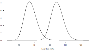
What could be the distribution of next year's loss ratio?

We can model this problem by assuming that the actual random process yields a log­normally distributed loss ratio $L$:

$\log \left(\text{L}\right)\sim N\left(\mu ,\sigma \right).$

For σ we represent our beliefs using the constant 0.25, so that no matter what μ is, l is usually between 0.75μ and 1.25μ. If μ is close to the 70% mean, then this implies a typical range of 0.75 $\times$ 70% = 52.5% to 1.25 $\times$ 70% = 87.5%, which is similar to the 70% $\pm$ 20% range of our beliefs.

For μ, we need to recognize that the true loss ratio is unknown, but we believe it to be 70% $\pm$ 10%. A simple way to model this belief is by assuming the true median loss ratio, $e^{\mu }$, is itself lognormally distributed with mean 70% and standard deviation 10%. Then

$\log \left(e^{\mu }\right)\mu \sim N\left({\mu }_0,{\sigma }_0\right),$

where ${\mu }_0$= -0.367 and ${\sigma }_0$= 0.142. Because ${\mu }_0$ and ${\sigma }_0$ determine a distribution ofμ, and μ itself parametrizes a distribution, ${\mu }_0$ and ${\sigma }_0$ are hyperparameters. Using hyperparameters is common in Bayesian statistics because we frequently have beliefs about what the actual parameters of some process might be.

Using the terminology of the previous section, the equations above determine our prior probability function P(x). Now we need to conditionalize on our evidence e (the historical loss ratios) to determine our posterior beliefs ${\mathbb{P}}_e\left(x\right)=\mathbb{P}\left(x|e\right).$

To calculate the posterior distribution of μ, we can us Bayes' theorem. It has a variety of statements, but this version is common for propositions and discrete variables, where T can be thought of as standing for “theory” and e for “evidence.”

$\mathbb{P}\left(T|e\right)=\frac{\mathbb{P}\left(e|T\right)\mathbb{P}\left(T\right)}{\mathbb{P}\left(e\right)}=\frac{\mathbb{P}\left(e|T\right)\mathbb{P}\left(T\right)}{\sum {}_{i=1}^n\mathbb{P}\left(e|T_i\right)\mathbb{P}\left(T_i\right)}.$

for continuous variables, the following version is more common. θ can be a scalar or a vector, and usually represents parameters to a theory or distribution.

$p\left(\theta |e\right)=\frac{p\left(e|\theta \right)p\left(\theta \right)}{p\left(e\right)}=\frac{p\left(e|\theta \right)p\left(\theta \right)}{\int p\left(e|\varphi \right)p\left(\varphi \right)d\varphi },$

All versions of Bayes' theorem follow from basic probably and the definition of conditional probability.

In this case, Bayes' theorem implies that our posterior distribution for μ is given by

$p\left(\mu |e\right)=\frac{p\left(e|\mu \right)p\left(\mu \right)}{\int p\left(e|\varphi \right)p\left(\varphi \right)d\varphi },$

where e is now the five observed historical loss ratios. We can now theoretically solve this equation because $p\left(e|\mu \right)$ and $p\left(e|\varphi \right)$ are given by the lognormal distribution, and $p\left(\varphi \right)$ is normally distributed.

Luckily, the equation has a simple solution in this case. Because our prior probability for μ is normal, and the likelihood of each loss ratio e (on a log-scale) given μ is also normal, the posterior distribution for μ is also normal, no matter what e is. When the prior and posterior are guaranteed to be in the same family, they are known as conjugate distributions or Bayesian conjugates. There are two other reasons this is convenient:

1. The posterior will remain in the same family as the prior when one data point is observed. Thus, this reasoning can be repeated to show that the posterior stays in the same family after any number of observations.
2. The parameters of the posterior distribution are typically simple functions of the parameters of the prior distribution and the observed data.

Our problem is an example of the normal/normal conjugate pair. See Table 3.2 for a table of conjugate pairs and their equations. In the normal/normal case, under the posterior probability distribution,

${\mu }_1\sim N\left({\left(\frac{1}{{\sigma }_0^2}+\frac{5}{{\sigma }^2}\right)}^{-1}\left(\frac{{\mu }_0}{{\sigma }_0^2}+\frac{1}{{\sigma }^2}\sum _{i=1}^5\log \left(r_i\right)\right),{\left(\frac{1}{{\sigma }_0^2}+\frac{5}{{\sigma }^2}\right)}^{-1}\right),$

where $r_i$ represents the five observed loss ratios. The posterior mean of μ is ${\mu }_1$ = -0.113. and the posterior standard deviation is ${\sigma }_1$ = 0.0879. The situation can be represented graphically in the chart. The observed loss ratios are marked with vertical lines. Here is the set of prior parameters:

> sigma <- .25

> prior.mean <- .7

> prior.sd <- .1

> sigmaO <- sqrt(log((prior.sd / prior.mean)^2 + 1))

> muO <- log(prior.mean) - prior.sd^2/2

Record observations are here:

> r <- c(0.958, 0.614, 0.977, 0.921, 0.756)

> n <- length(r)

Using previous discussion, we can compute posterior probabilities

> sigmal <- (sigma0^-2 + n / sigma^2)^-.5

> mul <- (mu0 / sigma0^;-2 + sum(log(r)) / sigma^2) * sigma1^2}

Those distribution can be visualized using

u <- seq (from = 0.3, to = 1.3, by = 0.01)

> prior <- dlnorm(u,mu0,sigma0)

> posterior <- dlnorm(u,mu1,sigma1)

> plot(u,posterior,type="l",lwd=2)

> lines(u,prior,lty=2)

We conclude this example with a few observations:

• Our distribution around the true loss ratio μ
• increased after observing the 5 years of data. This was to be expected because the observed loss ratios were, in general, larger than our prior mean of 70%.
• The posterior distribution of the true loss ratio is narrower (has a smaller standard deviation). This was also to be expected—after observing the data, we know more, and thus our uncertainty about the true loss ratio has decreased.
• The conceptual distinction between the parameter and predictive distributions is quite important. The parameter distributions are distributions over the parameters to other distributions (μ in this case). If we want to predict new observations, we must use the predictive distribution. The parameter distribution only quantifies parameter risk.
• The predictive distributions are significantly more uncertain than the parameter dis­tributions. This is also quite intuitive—much of the variability in insurance losses is contributed by process risk.
• In this case, our posterior predictive distribution is actually more uncertain than our prior predictive distribution (32.9% versus 30.5%). Although there is less parameter risk, there is more process risk because of the larger expected loss ratio.

3.2.3 Black Swans and Bayesian Methodology

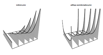
The use of Bayes's approach is interesting when you have no experience, at all. Consider the following simple case. Consider some Bernoulli sample, {0, 0,0,0,0}. What could you say about the probability parameter ? As a frequentist, nothing. This was actually the question asked to Longley-Cook in the 1950s: is it possible to predict the probability of two planes colliding in midair? There had never been any (serious) collision of commercial planes by that time. Without any past experience, statisticians could not answer that question.

Assume that $X_i\text{'}\text{s}$ are i.i.d. B(p) variables. With a beta prior for p, with parameters α andβ , then p given X has a beta distribution with parameters α and $\beta +5$ . Thus, with a flat prior $\left(\alpha =\beta =1\right)$ ,

> qbeta(.95,1,6)

[1] 0.3930378

the 95% confidence interval for p is [0%; 40%]. With Jeffrey's non-informative prior, (see Section 3.2.6.)

> qbeta(.95,.5,.5+5)

[1] 0.3057456

the 95% confidence interval for p is [0%; 30%]. It is possible to visualize the posterior trans­formation, with information coming, on Figure 3.3. For the uniform prior,

> pmat =persp(0:5,0:1,matrix(0,6,2),zlim=c(0,5), ticktype=

+ "detailed",box=FALSE,theta=-30)

> title("Uniform prior",cex.main=.9)

> y=seq(0,1,by=.01)

> for(k in 0:5){

+ z=dbeta(y,1,1+k)

+ indx=which(y<=qbeta(.95,1,1+k))

+ xy3d=tranS3d(rep(k,2*length(indx)),c(rev(y[indx]),y[indx]),

+ c(rep(0,length(y[indx])),z[indx]),pmat)

+ polygon(xy3d,col="grey",density=50,border=NA,angle=-50)

+ xy3d=tranS3d(rep(k,length(y)),y,z,pmat)

+ lines(xy3d,lwd=.5)

+ xy3d=tranS3d(rep(k,length(indx)),y[indx],z[indx],pmat)

+ lines(xy3d,lwd=3)}

To get back to the airplane collision, in 1955, Longley-Cook predicted “anything from 0 to 4 [...] collisions over the next ten years,” without any experience at all (so purchasing reinsurance might be a good idea). Two years later, 128 people died over the Grand Canyon, and 4 years after that, more than 133 people died over New York City.

3.2.4 Bayesian Models in Portfolio Management and Finance

Following Frost & Savarino (1986), it is possible to use a Bayesian methodology to discuss portfolio selection (see Chapter 13 for more details). Consider one assset, and a monthly sequence of returns for a given asset (a time series, see Chapter 11), r = (r1,...,rT). Let μ and σ denote the mean and the volatility of that return. Assume that returns are independent draws from a Gaussian distribution, $f\left(r|\mu \right)$ . Consider the conjugate prior, $\mu \sim N\left({\mu }_0,{\tau }_0\right)$ . Then the posterior distribution is Gaussian, $N\left({\mu }_T,{\tau }_T\right)$ , where

${\mu }_T=\left(\frac{{\mu }_0}{{\tau }_T^2}+\frac{T}{s^2}\frac{1}{T}\sum _{t=1}^T{r}_i\right){\left(\frac{1}{{\tau }_T^2}+\frac{T}{s^2}\right)}^{-1},$

Where

${\tau }_T^2={\left(\frac{1}{{\tau }_T^2}+\frac{T}{s^2}\right)}^{-1}.$

The posterior mean ${\mu }_T$ is here a weighted average of the priori mean ${\mu }_0$ and the historical average Observe that the less volatile the information, the greater its precision. And as more data become available, the prior information becomes increasingly irrelevant (and the posterior mean approaches the historical average).

Of course, it is possible to extend that model in higher dimension, with multiple assets. Consider a series of monthly returns, $\left(r_1,\mathrm{....},r_T\right)$ . Let μ and $\sum$ denote the vector of means, and the volatility matrix, of those returns. Assume that returns are independent draws from a Gaussian distribution, $f\left(r|\mu \right)$ . Consider the conjugate prior for the means $\mu \sim N\left({\mu }_0,{\tau }_0\right)$ . Here, ${\tau }_0$ reflects our priors on the covariance of the means, not the covariance of the asset returns. Actually, we can also consider priors on the covariance of the returns, too. The prior distribution of the covariance matrix has an inverse Wishart distribution, with v degrees of freedom, $\sum \sim IW\left(v,{\sum }_0\right)$ . Then the posterior distribution is Gaussian, $N\left({\mu }_T,{\sum }_T\right)$ where

${\mu }_T={\left({\tau }_0^{-1}+T{\widehat{\Sigma }}^{{}^{-1}}\right)}^{-1}\left({\tau }_0^{-1}{\mu }_0+{\widehat{\Sigma }}^{{}^{-1}}T\widehat{\mu }\right)$

and

${\sum }_T=\frac{T+1+v}{T+v-d-2}\left(\frac{v}{v+T}{\sum }_0\frac{T}{v+T}\widehat{\Sigma }\right),$

where d is the number of assets considered. Posterior means and covariances are linear mix­tures between the prior and the empirical (historical) estimates. If we have non-informative prior $v=0{\text{ and τ}}_0^{-1}=0,$ then

${\mu }_T=\widehat{\mu }\text{ and}{\sum }_T=\frac{T+1}{T-d-2}\widehat{\Sigma }.$

An extension is the so-called Black-Litterman model, introduced in Black & Litterman (1992) and discussed in Satchell & Scowcroft (2000). This model is popular among actuaries (and more generally investors) because it allows one to distinguish forecasts from conviction (or beliefs) about uncertainty associated to the forecast. This model will be discussed in Chapter 13.

3.2.5 Relation to Biihlmann Credibility

In the credibility framework, we assume that insurance portfolios are heterogeneous. There is an underlying (and non-observable) risk factor θ, for all insured, and we would like to model individual claim frequency for ratemaking issues. Let $Y_{i,t}$ denote the number of claims for year t and insurer i. In Chapters 14 and 15, the goal will be to use covariates $X_{i,t}$ as a proxy of ${\theta }_i$ and to use $\text{?}\left(Y_{i,t+1}|X_{i,t}\right)$ as an approximation for $\text{?}\left(Y_{i,t+1}|{\theta }_i\right)$. Here, instead of using covariates, we would like to use past historical observations. Namely, use $\text{?}\left(Y_{i,t+1}|Y_{i,t}\right)$ before as an approximation for $\text{?}\left(Y_{i,t+1}|{\theta }_i\right)$ where $Y_{i,t}=\left(Y_{i,t},Y_{i,t-1},Y_{i,t-2},\mathrm{...}\right)$ .

Consider a contract, observed during T years. Let $Y_t$ denote the number of claims, and assume that $Y_t\in \left\{0,1\right\}$ , so that $Y_t\sim B\left(p\right)$ . From the previous section, if we assume a priori beta distribution $B\left(\alpha ,\beta \right)$ for p, then

$\text{?}\left(p|Y\right)=\frac{\alpha +T{\overline{Y}}_T}{\alpha +\beta +T}=\frac{T}{\underset{Z}{\underbrace{\alpha +\beta +T}}}{\overline{Y}}_T+\underset{1-Z}{\underbrace{\left(1-\frac{T}{\alpha +\beta +T}\right)}}\underset{\text{?}\left(p\right)}{\underbrace{\frac{\alpha }{\alpha +\beta },}}$

where $Z\in \left[0,1\right]$,Because

$\text{?}\left(Y_t|p\right)=p\text{ and Var}\left(Y_t|p\right)=p\left(1-p\right),$

Then

$\begin{array}{cc}\frac{\text{?}\left(\text{Var}\left(Y_t|p\right)\right)}{\text{Var}\left(\text{?}\left(Y_t|p\right)\right)}& =\frac{\text{?}\left(p\left(1-p\right)\right)}{\text{Var}\left(p\right)}\hfill \\ & =\frac{\text{?}\left(p\right)-\left[\text{Var}\left(p\right)\text{+?}{\left(p\right)}^2\right]}{\text{Var}\left(p\right)}=\alpha +\beta \hfill \end{array}$

Thus,

$Z=\frac{T}{\alpha +\beta +T}=\frac{T}{k+T}\text{with}k=\frac{\text{?}\left(\text{Var}\left(Y_t|p\right)\right)}{\text{Var}\left(\text{?}\left(Y_t|p\right)\right)}.$

This will be known as the Bühlmann credibility approach: If insured i was observed T years, with past experience $Y_T=\left(Y_1,\mathrm{...},Y_T\right)$ , then $\text{?}\left(Y_{T+1}|Y_T\right)$ can be approximated by

$Z{\overline{Y}}_{i,T}+\left(1-Z\right)\mu ,\text{where}{\overline{Y}}_T=\frac{1}{T}\sum _{t=1}^T{Y}_{i,t},$

and μ, is the average on the whole portfolio. Z is then the share of the premium that is based on past information for a given insured, and is related to the amount of credibility we give to past information. From Biihlmann (1969), inspired by the Bayesian approach described previously, Z satisfies

$Z=\frac{T}{T+k}\text{where}k=\frac{\text{?}\left(\text{Var}\left(Y_t|\theta \right)\right)}{\text{Var}\left(\text{?}\left(Y_t\theta \right)\right)}.$

As mentioned in Bühlmann & Gisler (2005), in a Bayesian model, we wish to compute $\text{?}\left(Y_{T+1}|Y_T\right)$ , but here, we restrict ourselves to projections on linear combinations of past experience. We can actually prove that this Buhlmann credibility estimator is the best linear least-squares approximation to the Bayesian credibility estimator. And when $X_{i,t}\text{'}s$ are i.i.d. random variables in the exponential family, and if the prior distribution of θ is conjugate to this family, then Biihlmann credibility estimator is equal to the Bayesian credibility estimator. This was the case previously, where $X_{i,t}\text{'}s$ were Bernoulli and θ has a beta prior. Another popular example is obtained when $X_{i,t}\text{'}s$ are Poisson and θ has a gamma prior.

In order to illustrate Biihlmann credibility, consider claim counts, from Norberg (1979), $Y_{i,t}$ for contract i = 1,..., m and time t = 1,..., T.

> norberg

  year00 year01 year02 year03 year04 year05 year06 year07 year08 year09

 [1,]  0  0  0  0  0  0  0  0  0  0

 [2,]  0  0  0  0  0  0  0  0  0  0

 [3,]  1  0  1  0  0  0  0  0  0  0

 [4,]  0  0  0  0  0  0  0  0  0  0

 [5,]  0  0  0  0  0  1  0  0  1  0

 [6,]  0  0  0  0  0  0  0  0  0  0

 [7,]  0  1  1  0  0  0  0  0  0  0

 [8,]  0  0  0  0  0  0  0  0  0  0

 [9,]  0  1  1  0  1  1  1  0  0  1

[10,]  0  0  1  0  0  0  0  0  0  0

[11,]  1  1  0  0  1  0  0  0  1  0

[12,]  0  0  0  0  0  1  0  1  0  1

[13,]  0  0  0  0  0  0  0  0  1  0

[14,]  0  0  0  0  0  0  0  1  0  0

[15,]  0  0  0  0  0  0  0  0  0  0

[16,]  0  0  0  0  0  0  0  0  0  0

[17,]  1  1  0  1  0  0  1  0  0  1

[18,]  1  0  0  0  0  0  0  0  0  0

[19,]  0  0  0  0  0  0  0  0  0  1

[20,]  0  0  0  0  0  0  0  0  0  0

For each contract, we wish to predict the expected value $X_{i,T+1}$ given past observations. Bühlman's estimate is

$Z\cdot {\overline{Y}}_i+\left(1-Z\right)\overline{Y},\text{with}\frac{T}{T+k^{,}}$

where

${\overline{Y}}_i=\sum _{t=1}^T{Y}_{i,t}\text{while }\overline{Y}=\sum _{i=1}^m{\overline{Y}}_i,$

and where $k=s^2/a,$

$s^2=\frac{1}{m\left(T-1\right)}\sum _{t=1}^m\sum _{t=1}^T{\left(X_{i,t}-{\overline{X}}_i\right)}^2,$

and

$a=\frac{T}{m-1}\sum _{i=1}^m{\left({\overline{X}}_i-\overline{X}\right)}^2-\frac{1}{n}{s}^2;$

see Herzog (1996) for a discussion of those estimators. The code to compute Bühlman's estimate for year 11 will be:

> T<- ncol(norberg)

> (m <- mean(norberg))

[1] 0.145

> (s2 <- mean(apply(norberg,1,var)))

[1] 0.1038889

> (a <- var(apply(norberg,1,mean))-s2/T)

[1] 0.02169006

Bühlman's credibility factor is based on

> (Z <- T/(T+s2/a))

[I]    0.6761462

and Bühlman's estimates are

> Z*apply(norberg,1,mean)+(1-Z)*m

 [1]  0.0469588   0.0469588   0.1821880   0.0469588   0.1821880

 [6]  0.0469588   0.1821880   0.0469588   0.4526465   0.1145734

[II]  0.3174173   0.2498027   0.1145734   0.1145734   0.0469588

[16]  0.0469588   0.3850319   0.1145734   0.1145734   0.0469588

3.2.6 Noninformative Priors

In the first part of this section, we will use conjugate priors because of computational ease. As we will see in the next section, not having simple analytical expression is not a big deal. So it can be interesting to have more credible priors, even if it is not a simple problem, as discussed formally in Berger et al. (2009).

A simple example to start with can be the case where X given θ has a Bernoulli distribu­tion. As we have seen previously, on births, the idea of Pierre Simon Laplace was to assume a uniform prior distribution, $\pi \left(\theta \right)=1.$ Assuming $\pi \left(\theta \right)\propto 1$ (for more general distribution) will be called a flat prior. If Pierre-Simon Laplace thought it would be as neutral as possible, or non-informative, this is actually not the case. A more modern idea of formalizing the idea of non-informative priors (see Yang & Berger (1998) for a discussion) is that we should get an equivalent result when considering a transformed parameter. Given some one-to-one transformation h(), so that the parameter is no longer θ , but $\tau =h\left(\theta \right),$ , we want here to have invariant distributions. More formally, recall that the density of $\mathit{\text{τ}}$ is here

$p\left(\tau \right)=\pi \left(\theta \right).\left|\frac{\partial \theta }{\partial \tau }\right|.\text{(3.1)}$

Recall that this Jacobian has an interpretation in terms of information, as Fisher information of $\mathit{\text{τ}}$ is

$I_{\left(\tau \right)}=-?\left(\frac{{\partial }^2\log f\left(x|\tau \right)}{\partial {\tau }^2}\right)=I\left(\theta \right).{\left|\frac{\partial \theta }{\partial \tau }\right|}^2.$

Equation (3.1) can then be written as $p\left(\tau \right)\sqrt{I\left(\tau \right)}=\pi \left(\theta \right)\sqrt{I\left(\theta \right)}.$ Thus, it is natural to have a prior density which is proportional to the square root of Fisher information,

$\pi \left(\theta \right)\propto \sqrt{I\left(\theta \right)}.$

This is called Jeffrey's principle. For the Poisson distribution, it means that $\pi \left(\theta \right)\propto {\theta }^{-\frac{1}{2}},$ and if we get back to the initial problem, on births, the non-informative prior will be a beta distribution with parameters 1/2, as

$\pi \left(\theta \right)\propto \sqrt{\theta {\left(\frac{1}{\theta }-\frac{0}{1-\theta }\right)}^2+\left[1-\theta \right]{\left(\frac{0}{\theta }-\frac{1}{1-\theta }\right)}^2}=\frac{1}{\sqrt{\theta \left(1-\theta \right)}}.$

3.3 Computational Considerations

In many applications, we wish to compute

$?\left(g\left(\theta \right)|x\right)=\frac{\int g\left(\theta \right){\pi }^{\ast }\left(\theta |x\right)d\theta }{\int {\pi }^{\ast }\left(\theta |x\right)d\theta },$

where ${\pi }^{\ast }$ is proportional to the posterior density. One possible method is to use the Gauss- Hermite approximation, discussed in Klugman (1992) in detail. An alternative is based on Monte Carlo integration (see Chapter 1 for an introduction).

3.3.1 Curse of Dimensionality

Unfortunately, aside from Bayesian conjugates, most Bayesian problems are hard to com­pute. The problem is that the posterior distribution is often continuous and multidimen­sional and has the format

$\frac{p\left(e|\theta \right)p\left(\theta \right)}{\int p\left(e|\varphi \right)p\left(\varphi \right)d\varphi }$

for n-dimensional vector θ. Although $p\left(e|\theta \right)p\left(\theta \right)$ are often easy to compute, the normalizing constant $\int p\left(e|\varphi \right)p\left(\varphi \right)d\varphi$ is an n-dimensional integral. Typically, unless conjugate distribu­tions are used, this integral is not analytically soluble and must be approximated numeri­cally.

Here, Bayesian statistics suffer from the curse of dimensionality: the rapid increase in computational difficulty of integration as the number of dimensions increases.

In general, if we need to integrate a function over the d-dimensional unit hypercube ${\left[0,1\right]}^d,$ then this thinking suggests that we will need about ${100}^d$ evaluations. Thus, the number of function [calls] will increase quickly with dimensionality. Computers are much faster than they used to be, but even moderately small problems become computationally infeasible.

There are numerical integration algorithms such as Gaussian quadrature which can reduce the number of points required somewhat, but their error still decreases at the slow rate of $O\left(d^{-\frac{1}{n}}\right).$ . To make matters worse, Bayesian posterior probability distributions are often “spiky” (i.e. they have large areas with low probability and relatively small areas with lots of probability) like the distributions shown in Figure 3.1.

From a computational point of view, our interest is to approximate the value of an integral, which is an area for an $ℝ\to ℝ$ function, or a volume for an ${ℝ}^d\to ℝ$ function. A simple idea is to use a box, around the volume, to partition the box, and to count the proportion of points in the considered volume. For instance, to compute the area of a disk with radius 1, consider a box $\left[-1,+1\right]\times \left[-1,+1\right],$ , and compute the proportion of points on a grid in the box that belongs to the disk,

+ diskincube <- function(n){

+ gridn <- seq(-1,+1,length=n)

+ gridcube <- expand.grid(gridn,gridn)

+ inthedisk <- apply(gridcube"2,1,sum)<=1

 + mean(inthedisk)

+}

> diskincube(200)

[1] 0.7766

Here, 77.66% of the points in the square belong to the disk, and because the area of the cube is 22, it means that the area of the disk should be close to

> diskincube(200)*2^2

[1] 3.1064

> diskincube(2000)*2^2

[1] 3.138388

(the true value is $\pi$). Note that we always underestimate the true value with this technique. This method can be extended to higher dimensions. For instance, in dimension 4,

> diskincube.dim4 <- function(n){

+ gridn <- seq(-1,+1,length=n)

+ gridcube <- expand.grid(gridn,gridn,gridn,gridn)

+ inthedisk <- apply(gridcube^2,1,sum)<=1 

+ mean(inthedisk)

+}

The volume of the unit sphere in dimension 4 is larger than

> diskincube.dim4(40)*2^4 

[1] 4.4488

(the true value is ${\pi }^2/2~4.9348$)

More formally, we wish to estimate a volume $v\subset {ℝ}^d,\text{using }m=k^d$ points, for some integer k. If $v\in \left[a,b\right],$ , consider for any i a uniform partition of $\left[a_i,b_i\right]$ in k segments. Thus, define $x_{i,j}=a_i+\left(j-1\right)\left(b_i-a_i\right)/\left(k-1\right),\text{ for all }j\text{=}1,\mathrm{...},k.$ An approximation of volume v is then

$v\left(v\right)\sim \left(\prod _{i=1}^d{b}_i-a_i\right).\frac{1}{n}\sum _{j1,\mathrm{...},jd\in \left\{1,\mathrm{...},k\right\}}1\left(\left(x_{1,j1},\mathrm{...},x_{d,jk}\right)\in v\right)$

Let $V_n\left(v\right)$ denote this approximation. If $L\left(v\right)$ is the length of the contour of the volume, in dimension 2, then

$\left|V_n\left(v\right)-V\left(v\right)\right|\le \frac{L\left(v\right)}{k}=\frac{L\left(v\right)}{n^{1/d}}.$

The point here is that the approximation error is $O\left(1/n^{1/d}\right),$ , which will increase with di­mension.

This is more or less what we do when computing integrals,

${\int }_{\left[0,1\right]}h\left(u\right)du~\sum _{j=1}^n\frac{1}{n}.h\left(\frac{j}{n}\right)$

and in higher dimension,

${\int }_{{\left[0,1\right]}^d}h\left(u\right)du~\sum _{j_1,\mathrm{...},j_d\in \left\{1,\mathrm{...},k\right\}}{\left(\frac{1}{k}\right)}^d.h\left(\frac{j_1}{k},\mathrm{...},\frac{j_d}{k}\right).$

In dimension 1, we can prove that

$\left|{\int }_0^{1}h\left(u\right)du-\sum _{j=1}^n\frac{1}{n}\cdot h\left(\frac{j}{n}\right)\right|\le \frac{1}{2n}||f^{\text{'}}||\infty .$

and in higher dimension

$\left|{\int }_{{\left[0,1\right]}^d}h\left(u\right)du-\sum _{j_1,\mathrm{...},j_d}{\left(\frac{1}{k}\right)}^d.h\left(\frac{j_1}{k},\mathrm{...},\frac{j_d}{k}\right)\right|\le \frac{1}{n^d}||{\partial }^{d}f||\infty .$

Of course, this numerical algorithm can be improved, using trapezoids instead of rectangles, or Simpson's polynomial interpolation. But the order will remain unchanged, and the error is of order $O\left(1/n^{1/d}\right),$ . This is—more formally—what is called the curse of dimensionality.

3.3.2 Monte Carlo Integration

Now, if we get back to the initial example, it is possible to see what Monte Carlo methods are: Instead of considering a homogeneous grid, one idea can simply be to randomly draw n points, uniformly, in the box. An approximation of the volume will be

$V\left(v\right)\sim \left({\displaystyle \prod _{i=1}^d\left(b_i-a_i\right)}\right)\times \frac{1}{n}{\displaystyle \sum _{i=1}^{n}1\left(X_i\in v\right)}.$

Let ${\tilde{V}}_n\left(v\right)$ denote this approximation. To discuss and quantify errors, observe the fact that a point is, or is not, inside volume V can be modeled using Bernoulli random variables. It is then possible to prove that $?\left(V_n\left(v\right)\right)=V\left(v\right)$ and

$\text{Var}\left(V_n\left(v\right)\right)=\frac{1}{n}\times \frac{\left(V_n\left(v\right)\right)}{{\displaystyle \prod _{i=1}^d\left(b_i-a_i\right)}}\times \left(1-\frac{V\left(v\right)}{{\displaystyle \prod _{i=1}^d\left(b_i-a_i\right)}}\right).$

Now, this idea can be used to approximate integrals, as

${\int }_{{\left[0,1\right]}^d}h\left(u\right)du=?\left(h\left(U\right)\right)\text{where }U$ has independent components with $U_i~u\left(\left[0,1\right]\right),$ and from the law of large numbers

$\frac{1}{n}{\displaystyle \sum _{i=1}^{n}h\left(U_i\right)\underrightarrow{a.s.}?\left(h\left(U\right)\right).}$

To quantify uncertainty, define

$V_n=\frac{n}{n-1}\left(\frac{1}{n}{\displaystyle \sum _{i=1}^{n}h{\left(U_i\right)}^2-{\left(\frac{1}{n}{\displaystyle \sum _{i=1}^{n}h\left(U_i\right)}\right)}^2}\right),$

and from the central limit theorem, the error (in a more probabilistic way) is then of order $O\left(1/\sqrt{n}\right).$ . Note that the order does not depend on the dimension d here (actually, it does, in the constant term). Thus, Monte Carlo simulations can be more interesting in high dimension than deterministic methods.

> sim.diskincube.dim4(40"4)*2"4 

[1] 4.943763

(the true value is π2/2 ~ 4.9348). Recall that in using determinstic methods, we were still far from the true value

> diskincube.dim4(40)*2"4

 [1] 4.4488

To compare the deterministic algorithm and the Monte Carlo approach, we can plot the approximations obtained using the two algorithms (see Figure 3.4):

> v <- 1:40

> plot(v,2^4*Vectorize(sim.diskincube.dim4)(v"4),type="b",)

> lines(v,2^4*Vectorize(diskincube.dim4)(v),type="b",pch=19,cex=.6,lty=2)

> abline(h=pi"2/2,col="grey")

3.3.3 Markov Chain Monte Carlo

Currently the most popular way in Bayesian statistics to sidestep the curse of dimensionality is to use Markov Chain Monte Carlo (MCMC) techniques. Interestingly, the first MCMC technique, the Metropolis algorithm, was developed by the eponymous physicist in 1953. It was run on some of the very first computers.

Despite this early beginning, the Metropolis algorithm and related MCMC techniques only gained popularity in the statistical community in the 1990s. The resurgence of Bayesian statistics since then owes much to the effectiveness and practicality of these algorithms.

MCMC techniques do not even attempt to calculate the integral $\int p\left(e|\varphi \right)p\left(\varphi \right)d\varphi .$ . Rather, they provide samples of θ from the posterior distribution of $p\left(\theta |e\right).$ . MCMC techniques are Monte Carlo, meaning that they depend on random sampling, but they also produce Markov chains, meaning that the samples they produce are not independent. Each sample depends on the previous one.

The Metropolis algorithm uses the insight that we do not need to compute $\int p\left(e|\varphi \right)p\left(\varphi \right)d\varphi .$ to get samples; rather, we can work with the unnormalized probability distribution $p\left(e|\theta \right)p\left(\theta \right)$ , which is usually easy to compute. The algorithm can be informally summarized like this:

1. Start with an arbitrary value in the posterior distribution ${\theta }_0$ .
2. Given an existing sample ${\theta }_i$ , randomly choose a “nearby” candidate sample $\theta \text{'}$ . This is done by sampling from another probability distribution $Q\left(\cdot |{\theta }_i\right).$ Often, Q is chosen to be multinormal, so that $\theta \text{'}~N\left({\theta }_i,\Sigma \right),$ , for some fixed $\sum$ .
3. Compare $p\left(e|{\theta }_i\right)p\left({\theta }_i\right)\text{ and }p\left(e|\theta \text{'}\right)p\left(\theta \text{'}\right)$ by computing the acceptance ratio

   $R=\frac{p\left(e|\theta \text{'}\right)p\left(\theta \text{'}\right)}{p\left(e|{\theta }_i\right)p\left({\theta }_i\right)}.$

4. Move to $\theta \text{'}$ if R is big enough: with probability min(1,R) set ${\theta }_{i+1}=\theta \text{'}$ (this is called accepting $\theta \text{'}$); with probability 1 — min(1,R) set ${\theta }_{i+1}={\theta }_i$ (this is called rejecting $\theta \text{'}$).
5. Go to step (2) and continue until enough samples are drawn.

This chapter will not prove that the samples thus drawn can be considered samples from the posterior distribution $p\left(\cdot |e\right).$ However, it is hopefully clear from the algorithm that it will spend more time where $p\left(e|\theta \text{'}\right)p\left(\theta \text{'}\right)$ is large and less time where it is small. This is because the acceptance ratio will always be 1 when the candidate moves us into an area of higher probability. When the candidate sample moves us into an area of lower probability, the acceptance ratio will be less than 1 and we may just stay where we are. Because $p\left(e|\theta \text{'}\right)p\left(\theta \text{'}\right)$ is large in exactly the same places that the posterior distribution

$p\left(\theta \text{'}|e\right)=\frac{p\left(e|\theta \text{'}\right)p\left(\theta \text{'}\right)}{\int p\left(e|\varphi \right)p\left(\varphi \right)d\varphi }$

is large, more samples will be drawn from the areas of probability space where the posterior density is large.

Once we have samples from the posterior distribution, we can estimate the answer to most questions that come up in Bayesian statistical problems. For instance, suppose we have n samples of θ and want to know the expected value of the first parameter ${\theta }_0$ . Then we can use classical statistics to approximate it:

$?\left({\theta }_0\right)\approx \frac{1}{n}{\displaystyle \sum _{i=1}^n{\theta }_{0,i}}.$

It is ironic but many or most Bayesian techniques in the end depend on classical statistics to understand the behavior produced by MCMC chains.

3.3.4 MCMC Example in R

Let us examine a simple Bayesian problem that cannot be solved using Bayesian conjugates, but can be quickly analyzed with an MCMC technique. Recall the example in Section 3.2. The goal was to find the posterior mean and standard deviation (parameter risk) of the expected loss ratio. We assumed there that the process risk was lognormally distributed with fixed σ= 0.25, thus overlooking an opportunity to learn about our process risk from the data.

This time let us use the same numbers but model uncertainty aboutσ. We will again assume that the process risk of actual loss ratios is lognormally distributed, with parameters μand σ. The prior distribution of u will again be normally distributed with the same parameters ${\mu }_0$ and ${\sigma }_0$ . However, now our prior distribution of a will be inverse gamma with parameters $k_0\text{ and }{\theta }_0.$ (σ cannot be negative, so the inverse gamma distribution is commonly used to model a prior variance distribution). We can set $k_0\text{ and }{\theta }_0.$ using the method of moments.

> prior.mean.mean <- .7

> prior.mean.sd <- .1

> prior.sd.mean <- .25

> prior.sd.sd <- .1

Using the fact that for a lognormal distribution, the coefficient of variation is $\sqrt{(}{e}^{s^2}-1)$,

> sigmaO <- sqrt(log((prior.mean.sd / prior.mean.mean)"2 + 1))

> mu0 <- log(prior.mean.mean) - sigma0"2 / 2

and for an inverse Gamma distribution, $E\left(X\right)=\frac{\Theta }{\left(k-1\right)}$ and the coefficient of variation is $\frac{1}{\sqrt{k-2}},$

> kO <- 2 + (prior.sd.mean / prior.sd.sd)"2

> thetaO <- (kO - 1) * prior.sd.mean

Record observations are here

> r <- c(0.958, 0.614, 0.977, 0.921, 0.756)

> r.log <- log(r)

> n <- length(r)

In order to use the dinvgamma() function, use

> library{MCMCpack}

The code to run MCMC simulations is here

> RunSim <- function(M, delta, mu, sigma) {

+  output.df <- data.frame(mu=rep(NA, M), sigma=NA)

+  set.seed(0)

+  cur.prior.log <- (dnorm(mu, mu0, sigma0, log=TRUE)

+    + log(dinvgamma(sigma, k0, theta0)))

+  cur.like.log <- sum(dnorm(r.log, mu, sigma, log=TRUE))

+  for (i in seq_len(M)) {

+    mu.cand <- mu + rnorm(1, sd=delta)

+   sigma.cand <- max(1e-5, sigma + rnorm(1, sd=delta/2))

+   cand.prior.log <- (dnorm(mu.cand, mu0, sigmaO, log=TRUE)

+  + log(dinvgamma(sigma.cand, k0, theta0)))

+    cand.like.log <- sum(dnorm(r.log, mu.cand, sigma.cand, log=TRUE))

+    cand.ratio <- exp(cand.prior.log + cand.like.log

+   - cur.prior.log - cur.like.log)

+  if (runif(1) < cand.ratio) {

+  mu <- mu.cand

+  sigma <- sigma.cand

+  cur.prior.log <- cand.prior.log

+  cur.like.log <- cand.like.log

+  }

+   output.df[i,] <- c(mu, sigma) # write one sample to output

+  }

+ return(output.df)

+}

> delta005.df <- RunSim(6000, .005, log(1.2), 0.5)

> delta20.df <- RunSim(6000, .20, log(1.2), 0.5)

> delta80.df <- RunSim(6000, .80, log(1.2), 0.5)

The comments in the code largely explain what is happening. Lines here compute the acceptance ratio

$R=\frac{p\left(e|\theta \text{'}\right)p\left(\theta \text{'}\right)}{p\left(e|{\theta }_i\right)p\left({\theta }_i\right)}.$

and line 49 updates the current values for μ and σ by moving only if the acceptance ratio is high enough. Note that the step size delta ($\delta$), the number of samples to run M, and the starting values are purely computational decisions—they are not determined by the probabilistic structure of the problem—so above we have made them functional inputs.

The last few lines run three simulations, each with 6,000 samples. The three use the same arbitrarily chosen inputs; the difference between the three is the step size $\delta$ .Examining the three output dataframes, we find that the acceptance ratio when $\delta$ =.005 is about 95%; when $\delta$ = 0.10, it is 26%, and when J = 0.80, it is only 2.4%. The following graphs in Figure 3.5 of the first samples from each simulation illustrate the phenomenon. These are sometimes called traceplots. They can be obtained using

> library(coda)

> traceplot(mcmc(delta20.df[1001:6000,]))

for instance, or

> lr <- function(m) exp(m[,1] + .5*m[,2]"2)

> lrsd <- function(m) sqrt((exp(m[,2]"2)-1)*exp(2*m[,1]+m[,2]"2))

> plot(100*lr(delta005.df[1001:6000,]),type="l",ylim=c(62,145),

+ ylab="Mean of Loss Ratio (in %)")

> abline(h=100,col="grey",lty=2)

> plot(100*lrsd(delta005.df[1001:6000,]),type="l",ylim=c(0,75),

+ ylab="Std. Dev. of Loss Ratio (in %)")

The goal of our simulation is to crawl around probability space so that we reach all the important parts of the space, and that the length of time we spend there is proportional to $p\left(e|\theta \right)p\left(\theta \right)$ . When $\delta$ = 0.005, we are moving too slowly through the space, and it takes us a long time (many processor cycles) to travel around. When $\delta$ = 0.8, our jumps are too big and keep getting rejected, so we again do not travel efficiently. $\delta$ = 0.2 achieves an acceptance ratio of 26%, which looks reasonable. Indeed, theoretical results suggest that acceptance ratios in the 20%-50% range are optimal. An MCMC simulation that is sampling efficiently from the posterior distribution is said to have good mixing.

Another detail to consider before using the output is the initial value of p and a. Ideally, the starting values would have high posterior probability, but typically this information is not available as learning the posterior probability is the whole point of the MCMC calculation. Instead, the starting values often have very low probability, as in the case in this example. If we included the starting samples, the initial probabilities would get too much weight. We can fix this by excluding the first part of the chain. These discarded results are often called burn-in samples. From the graphs we can see that the 6 = 0.2 simulation has burned in after 1,000 samples, so we will only use samples 1001-6000 in our analysis.

A final detail to worry about when using MCMC techniques is convergence. Because we are using a Monte Carlo technique, any answers provided will only be asymptotically correct, and the error may be very large if we do not use enough samples. Because MCMC samples will be autocorrelated, one approach is to fit a simple time series to the simulation results and estimate the error using results proven about time series. This can be done using the coda package in R:

> library(coda)

> summary(mcmc(delta20.df[1001:6000,]))

Below are the coda results. Note that the time series error estimate is almost three times higher than the “naive” error estimate because of autocorrelation; much higher ratios are possible. This is important to keep in mind. Do not just assume that your error is low because you have 100,000 samples, because they might just be equivalent to 100 truely independent samples!

Iterations = 1:5000

Thinning interval = 1 

Number of chains = 1 

Sample size per chain = 5000

1. Empirical mean and standard deviation for each variable,
  plus standard error of the mean:

   Mean  SD   Naive SE   Time-series SE

mu  -0.2450  8.387e-02   1.186e-03   0.003176

sigma 0.2220  5.754e-02   8.138e-04   0.002783

2. Quantiles for each variable:

   2.5%  25%  50%  75% 97.5%

mu  -0.4160 -0.3013 -0.2452 -0.1848 -0.08963

sigma 0.1354  0.1801  0.2116  0.2527  0.35980

Although mixing, burn-in are convergence important considerations when running MCMC analyses, they are still only “practical” issues. In theory, all of these simulations provided correct samples from the posterior distribution without burn-in, even if we start at a low (non-zero) probability region, and even if our mixing is slow. However, in practice, a problem with any of these issues can make MCMC results unusuable.

Aside from using the summary statistics produced by coda, we can use the samples of μ and σ directly. For instance, if we wanted to simulate future loss ratios in a way that reflected both process risk and parameter risk, we could do that by first sampling μ and σ from delta20.df and then drawing from a lognormal distribution with those parameters.

3.3.5 JAGS and Stan

The previous subsection was hopefully instructive, but it is usually a mistake to hand-code MCMC algorithms in R for practical projects. There are a few reasons for this:

1. It can be difficult to choose the step size, especially with high-dimensional prob­lems. Notice above that I judgmentally set the σ step size to be half of the μ step size. In practice, all the dimensions may be different sizes, and the optimum step size may even be a function of the region of probability space.
2. There are better versions of the Metropolis algorithm exhibited above. The Metropolis-Hastings and Gibbs sampling algorithms are popular basic algo­rithms. More recently, there have been a variety of sophisticated algorithms pro­posed.
3. The R code can obscure the probabilistic structure of the problem—even with the simple Metropolis algorithm, there no very clear connection between the code and probabilistic assumptions. This gap would be even wider for a more complex algorithm.
4. R is slow for computations that cannot be vectorized, like the example above. It is not uncommon for a calculation coded in C/C++ to be 20 (or even 100) times faster than the equivalent coded in R; see Chapter 1.

To solve these problems, a few general-purpose MCMC engines have been developed.

The two described in this chapter are JAGS (Just Another Gibbs Sampler; see Plummer (2011)) and Stan (see Stan Development Team (2012), named after Stanislaw Ulam, one of the inventors of the Monte Carlo technique; see Metropolis & Ulam (1949)). Both of them allow you to specify your prior distribution and data in a special language designed for Bayesian statistics. They then analyze the probabilistic structure of the problem and design and run an MCMC algorithm tailored to solve it. The output is samples from the posterior distribution as in our manual example above. When it works, it is pretty magical.

This chapter will show and briefly explain sample JAGS and Stan code that solves the earlier Bayesian problem. Both JAGS and Stan come with extensive reference manuals, and example models for both are available online. However, both tools have a bit of a learning curve to install and use.

JAGS (see Plummer (2003))is an open-source, enhanced, cross-platform version of an earlier engine BUGS (Bayesian inference Using Gibbs Sampling). Here is sample JAGS code (interfaced to R using the runjags package) that computes the prior problem:

> library(runjags)

+ jags.model <- "

+ model {

+ mu ~ dnorm(mu0, 1/(sigma0^2))

+ g ~ dgamma(k0,theta0)

+ sigma <- 1 / g

+ for (i in 1:n) {

+  logr[i] ~ dnorm(mu, g^2)

+}

+}"

Then,

> jags.data <- list(n=n, logr=log(r), mu0=mu0, sigma0=sigma0,

+    k0=k0, theta0=theta0)

> jags.init <- list(list(mu=log(1.2), g=1/0.5^2),

+    list(mu=log(.8), g=1/.2^2))

> model.out <- autorun.jags(jags.model, data=jags.data, inits=jags.init,

+      monitor=c("mu", "sigma"), n.chains=2)

> traceplot(model.out$mcmc)

> summary(model.out)

The actual model code is very straightforward; the only complication is that there is no built-in inverse gamma function, and the JAGS normal distribution wants the spread quantified using the precision rather than the standard deviation. We compensate for that above by calculating precision from standard deviation and the inverse gamma from the gamma distribution.

Here is the output produced by the last line, which matches our manual Metropolis algorithm to within error:

Iterations = 5001:15000 

Thinning interval = 1 

Number of chains = 2 

Sample size per chain = 10000

1. Empirical mean and standard deviation for each variable,

  plus standard error of the mean:

    Mean  SD Naive SE Time-series SE

mu   -0.2439 0.08382 0.0005927  0.0006377

sigma  0.2264 0.06182 0.0004372  0.0005879

2. Quantiles for each variable:

   2.5%  25%  50%  75%  97.5%

mu  -0.4185 -0.2974 -0.2408 -0.1877  -0.08711 

sigma 0.1389  0.1830  0.2158  0.2575 0.37555

Stan, is a newer tool that uses the Hamiltonian Monte Carlo (HMC) sampler. HMC uses information about the derivative of the posterior probability density to improve mix­ing. These derivatives are supplied by algorithm differentiation, a neat computational trick for finding derivatives quickly. Unlike JAGS, which is interpreted, Stan produces C/C++ code which is then compiled by gcc (a standard open-source compiler). Stan is newer and less well tested than JAGS, and lacks a few features compared to JAGS (such as dealing with discrete distributions cleanly) but it works great on many problems and has a lot of potential.

Here is R code which uses Stan via the rstan package to solve our example:

> library(rstan)

> stan.model <- "

+ data {

+ int<lower=0> n; // number of data points

+ vector[n] r;  //observed loss ratios

+ real mu0;

+ real<lower=0>  sigma0;

+ real<lower=0>  k0;

+ real<lower=0>  theta0;

+}

+ parameters {// Values we want posterior distribution of

+  real mu;

+  real<lower=0> sigma;

+}

+ model {

+ mu ~ normal(mu0, sigma0);

+ sigma ~ inv_gamma(k0, theta0);

+ for (i in 1:n)

+ log(r[i])  ~ normal(mu, sigma);

+}"

...

> stan.data <- list(n=n, r=r, mu0=mu0, sigma0=sigma0, k0=k0, theta0=theta0)

> stan.out <- stan(model_code=stan.model, data=stan.data, seed=2)

> traceplot(stan.out)

> print(stan.out, digits_summary=2)

The traceplot line suggests that Stan's MCMC chains converge quickly and have good mixing. Here is the output produced by the last line:

Inference for Stan model: stan.model.

4 chains, each with iter=2000; warmup=1000; thin=1;

 post-warmup draws per chain=1000, total post-warmup draws=4000.

  mean  se_mean  sd  2.5%  25%  50%  75%  97.5%  n_eff  Rhat

mu  -0.25  0.00  0.08 -0.42 -0.30 -0.25 -0.19  -0.09  1648  1.00

sigma 0.23  0.00  0.06  0.14  0.19  0.22  0.26  0.39  1358  1.00

lp__ 8.64  0.03  1.06  5.77  8.23  8.96  9.39  9.67  1177  1.01

As you can see, the mean values for μ and a agree with our manual Metropolis algorithm to within error. The Stan MCMC samples also show better mixing than our attempt.

3.3.6 Computational Conclusion and Specific Packages

Despite the conceptual simplicity of Bayesian statistics, computing the posterior distribu­tions required by Bayesian statistics can still be an unfortunately complicated ordeal. This complexity has historically held Bayesianism back, but in recent decades the popularity of Bayesian statistics has been bolstered by increasing computer speed and the development of powerful MCMC algorithms and engines.

The options for computing Bayesian posteriors are usually ranked as follows in decreasing order:

1. Use a simple Bayesian conjugate if available,
2. Find an appropriate package such as MCMCpack or arm that implements the solution for you,
3. Write a custom model and let JAGS or Stan produce samples for you, and
4. As a last resort, write a custom sampler, perhaps using Rcpp for speed.

3.4 Bayesian Regression

To illustrate potential application of Bayesian methodology, let us describe Bayesian regres­sion (starting with the linear model, and discussing briefly Generalized Liner Models).

3.4.1 Linear Model from a Bayesian Perspective

In the standard Gaussian linear, we assume that $Y=X\beta +\epsilon ,$ , where $\epsilon$ is a Gaussian i.i.d. noise, centred, with variance ${\sigma }^2$ , where $X=\left(1,X_1,\mathrm{...},X_k\right).$ . The likelihood of this model, given a sample $\left\{\left(Y_i,X_i\right)\right\}\text{ for }i=1,\mathrm{...},n,$ is then

$L\left(\beta ,{\sigma }^2|Y,X\right)={\left[2\pi {\sigma }^2\right]}^{-\frac{n}{2}}\exp \left[-\frac{1}{2{\sigma }^2}{\left(Y-X\beta \right)}^{\text{T}}\left(Y-X\beta \right)\right].$

As mentioned in Chapter 2, maximum likelihood estimator ofβ is $\widehat{\beta }={\left(X^{\text{T}}X\right)}^{-1}{X}^{\text{T}}Y,$ , and an unbiased estimator of the variance parameter ${\sigma }^2$ is

${\widehat{\sigma }}^2=\frac{{\left(Y-X\beta \right)}^{{\rm T}}\left(Y-X\beta \right)}{n-k-1}=\frac{s^2}{n-k-1}.$

Observe that the likelihood can be written as

$L\left(\beta ,{\sigma }^2|Y,X\right)={\left[2\pi {\sigma }^2\right]}^{-\frac{n}{2}}\exp \left[-\frac{1}{2{\sigma }^2}{\left(Y-X\widehat{\beta }\right)}^{{\rm T}}\left(Y-X\widehat{\beta }\right)-\frac{1}{2{\sigma }^2}{\left(\beta -\widehat{\beta }\right)}^{{\rm T}}\left(X^{{\rm T}}X\right)\left(\beta -\widehat{\beta }\right)\right],$

or equivalently,

$L\left(\beta ,{\sigma }^2|Y,X\right)=\pi \left({\sigma }^2\right).\pi \left(\beta |{\sigma }^2\right),$

where the first distribution is an inverse gamma distribution, and the second is a multivariate normal with covariance matrix proportional to ${\sigma }^2$ . For computational ease, conjugate prior can be constructed with those families. More specifically, assume that prior distributions are

$\beta |{\sigma }^2~N\left({\beta }_0,{\sigma }^2{M}_0^{-1}\right),$

for some positive definite $\left(k+1\right)\times \left(k+1\right)$ symmetric matrix $M_0$ , while

${\sigma }^2~IG\left(a_0,b_0\right).$

In that case, the (conditional) posterior distribution of $\beta$ given ${\sigma }^2\text{ and }Y$ is

$\beta |{\sigma }^2,Y~N\left({\left[Mo+\left(X^{\top }X\right)\right]}^{-1}\left[M_o{\beta }_o+\left(X^{\top }X\right)\widehat{\beta }\right],{\sigma }^2{\left[Mo+\left(X^{\top }X\right)\right]}^{-1}\right)$

while the posterior distribution for σ2 is

${\sigma }^2|Y~IG\left(\frac{n}{2}{a}_0,b_0+\frac{{\left[{\beta }_0-\widehat{\beta }\right]}^{\top }{\left(M_0+\left(X^{\top }X\right)\right)}^{-1}\left[{\beta }_0-\widehat{\beta }\right]}{2}\right)$

With this framework, prior and posterior distributions are in the same family. Simple com­putations show that

$?\left(\beta |Y,X\right)={\left(M_0+|\left(X^{\top }X\right)\right)}^{-1}\left[\left(X^{\top }X\right)\widehat{\beta }+M_0{\beta }_0\right]$ .

and

$?\left({\sigma }^2|Y,X\right)=\frac{2b_0+s^2+{\left[{\beta }_0-\widehat{\beta }\right]}^{\top }{\left(M_0^{-1}+{\left(X^{\top }X\right)}^{-1}\right)}^{-1}\left[{\beta }_0-\widehat{\beta }\right]}{n+2\left(a_0-1\right)}$

The interesting point is that, since we have explicitly posterior distributions, it is possible to derive credibility intervals for parameters, as well as predictions, $\widehat{Y}$ for a given x. If we use the Bayesian Central Limit theorem (mentioned in the introduction of this chapter), and

$?\left(\widehat{Y}|Y,X\right)=x{\left[\left(X^{\text{T}}X\right)+M_0\right]}^{-1}\left[\left(X^{\text{T}}X\right)\widehat{\beta }+M_0{\beta }_0\right]$ and

$\mathrm{var}\left(\widehat{Y}|Y,X\right)={\sigma }^2\left(1+x{\left[\left(X^{\top }X\right)+M_0\right]}^{-1}{x}^{\top }\right),$

we get bounds for an approximated credibility interval.

To illustrate this model, consider the same example as in Section 2.4 in Chapter 2.

> Y <- Davis$height

> X1 <- Davis$sex

> X2 <- Davis$weight

> df <- data.frame(Y,X1,X2)

> X <- cbind(rep(1,length(Y)),(X1=="M"),X2)

> beta0 <- c(150,7,1/3)

> beta <- as.numeric(lm(Y~X1+X2,data=df)$coefficients)

> sigma2 <- summary(lm(Y~X1+X2,data=df))$sigma"2

> M0 <- diag(c(100,100,1000~2))

If we consider a prediction for a male with weight 70 kg,

> Xi <- c(1,1,70) 

then the prediction is

> (m <- Xi%*%solve(M0+t(X)%*%X) %*%((t(X)7.*7.X)7.*7.beta +M0°7*7.beta0))

  [,1]

[1,] 176.7536

and a 95% credibility interval based on the Gaussian approximation is

> s2 <- sigma2*(1+ (t(Xi)7*7 (solve(M0+t(X)7.*7.X)))7.*°7(Xi))

> qnorm(c(.025,.975),mean=m,sd=sqrt(s2))

[1] 166.6124 186.8947

Those values can be compared with the lower and upper bound obtained using function predict() (using σ standard statistical approach)

> predict(lm(Y~X1+X2,data=df),newdata=

+ data.frame(X1="M",X2=70),interval="prediction")

  fit  lwr  upr

1 176.057 165.8188 186.2951

3.4.2 Extension to Generalized Linear Models

In Generalized Linear Models (see McCullagh & Nelder (1989) or Chapter 14), two functions must be specified:

• The (conditional) distribution of Y given X, that belongs to the exponential family, and let f denote the associate density (or probability function for discrete variables)
• A link function g that relates the (conditional) mean $\mu \left(x\right)=?\left(Y\right|X=x)$ and the covariates, as $g\left(\mu \left(x\right)\right)=x^{\top }\beta$

This link function should be bijective, for identifiability reasons, and then, $\mu \left(x\right)=g^{-1}\left(x^{\top }\beta \right)$ .

Two popular models are the logit (or probit) and the Poisson models. In the logit model, Y is a binary response, $Y|X~B\left(\pi \left(X\right)\right),$ , where the link function is the logit transform, $g\left(x\right)=log\left[x/\left(1—x\right)\right]$ . An alternative is the probit model, where the link function is the quantile function of the $N\left(0,1\right)$ N(0,1) distribution, $g\left(x\right)={\varphi }^{-1}\left(x\right)$ . For the Poisson model, Y is a counting response, with a Poisson distribution $Y|X~P\left(\lambda \left(X\right)\right)$ , where the link function is the log transform, $g\left(x\right)=\text{ log}\left[x\right]$ .

The Probit Hastings-Metropolis sampler, in the context of a Probit model can be the fol­lowing: To initialize, start with maximum likelihood estimators, ${\beta }_{\left(0\right)}=\widehat{\beta }$ with (asymptotic) variance function matrix $\widehat{\Sigma }$ . At stage k,

1. Generate $\beta ~N\left({\beta }_{\left(k-1\right)},{\tau }^2\widehat{\Sigma }\right)$
2. With probability min, $\left\{1,\frac{\pi \left(\beta |Y\right)}{\pi \left({\beta }_{\left(k-1\right)}|Y\right)}\right\},\text{set }{\beta }_{\left(k\right)=\beta },\text{otherwise }{\beta }_{k-1}.$

A natural idea is to use a flat prior, so that the posterior distribution is

$\pi \left(\beta |Y\right)\propto {\displaystyle \prod _{i=1}^n\Phi {\left(X_i^{\top }\beta \right)}^{Y_i}{\left[1-\Phi \left(X_i^{\top }\beta \right)\right]}^{1-Y_i}.}$

Consider the attorney dataset, autobi (from Frees (2009)). We will consider here only fifty observations (with no missing values):

> index <- which((is.na(autobi$CLMAGE)==FALSE)&

+ (is.na(autobi$CLMSEX)==FALSE))

> set.seed(123)

> index <- sample(index,size=50)

The variable of interest is whether an insured got an attorney, or not,

> Y <- autobi$ATTORNEY[index]

Consider the following regression, where covariates are the cost of the claim, the sex of the insured and the age of the insured. The posterior density is here

> X <- cbind(rep(1,nrow(autobi)),

+ autobi$LOSS,autobi$CLMSEX==2,autobi$CLMAGE)

> X <- X[index,]

The posterior density is here

> posterior <- function(b)

+ prod(dbinom(Y,size=1,prob=pnorm(X%*%b)))

The Hastings-Metropolis alogrithm is here

> model <- summary(glm(Y~0+X,family=binomial(link="probit")))

> beta <- model$coeff[,1]

> vbeta <- NULL

> Sigma <- model$cov.unscaled

> tau <- 1

> nb.sim <- 10000

> library(mnormt)

> for(s in 1:nb.sim){

+ sim.beta <- as.vector(rmnorm(n=1,mean=beta,varcov=tau"2*Sigma))

+ prb <- min(1,posterior(sim.beta)/posterior(beta))

+ beta <- cbind(beta,sim.beta)[,sample(1:2,size=1,prob=c(1-prb,prb))]

+ vbeta=cbind(vbeta,beta)

+}

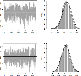
In order to visualize generated sequences, let us remove the first 10% and plot the sequence of ${\beta }_2$'s (parameter associated to the cost of the claim),

> mcmc.beta <- vbeta[,seq(nb.sim/10,nb.sim)]

> plot(mcmc.beta[2,],type="l",col="grey")

> abline(h=model$coeff[2,1],lty=2)

We can also visualize the distribution of the ${\beta }_2$'s:

> hist(mcmc.beta[2,],proba=TRUE,col='grey',border='white')

> vb <- seq(min(mcmc.beta[2,]),max(mcmc.beta[2,]),length=101)

> lines(vb,dnorm(vb,model$coeff[2,1],model$coeff[2,2]),lwd=2)

> lines(density(mcmc.beta[2,]),lty=2)

The plain line is the standard asymptotic Gaussian distribution (in GLMs, the distribution of the parameters is only asymptotic), and the dotted line, the kernel-based estimator. The code can also be used for the age variable, with sequence of ${\beta }_4\text{'}s$ ; see Figure 3.6.

3.4.3 Extension for Hierarchical Structures

In some applications, data are slightly more complex and might exhibit some hierarchi­cal structures. Consider the case where several companies wish to share their experience through an (independent) ratemaking bureau, in order to enhance the predictive power of all companies (as discussed in Jewell (2004)). Then observations are $\left(Y_i,X_i\right)$ , related to insured i, from company j. There might be market factors, company risk factors and in­dividual risk factors. Those models will be discussed in Chapter 15. Such complex models can be difficult to estimate using standard techniques, but a Bayesian approach can be extremely powerful.

Consider a simple linear model, where the intercept may vary by group,

$Y_i={\alpha }_{j\left[i\right]}+{\beta }_1{X}_{1,i}+{\beta }_2{X}_{2,i}+{\epsilon }_i.$

This is a fixed effects model, and it can be estimated using dummy variables. A more flexible alternative is to use a so-called hierarchical model, or multilevel model, also called mixed (or random) effects model. Here,

$Y_i={\alpha }_{j\left[i\right]}+{\beta }_1{X}_{1,i}+{\beta }_2{X}_{2,i}+{\epsilon }_i,\text{with }{\alpha }_j~N\left(\gamma ,{\top }^2\right).$

While previously we assumed that there were different intercepts for each group, now we assume that intercepts are drawn from an identical random variable. One can also write

$Y_i={\alpha }_{j\left[i\right]}+{\beta }_1{X}_{1,i}+{\beta }_2{X}_{2,i}+{\epsilon }_i,\text{with }{\alpha }_j=\alpha +{\eta }_j,$

and it is possible to incorporate group-level covariates, such as

$Y_i={\alpha }_{j\left[i\right]}+{\beta }_1{X}_{1,i}+{\beta }_2{X}_{2,i}+{\epsilon }_i,\text{with }{\alpha }_j={\gamma }_0+{\gamma }_1{Z}_{1,j}+{\gamma }_2{Z}_{2,j}+{\eta }_j,$

Using standard likelihood-based methods, this is a difficult model to estimate. But here, we can use a Bayesian model. Write here

$f\left(\alpha ,\beta ,\gamma |Y)\alpha f(Y|\alpha ,\beta ,\gamma \right)\cdot \pi \left(\alpha |\gamma \right)\pi \left(\gamma \right)\pi \left(\beta \right).$

And one can use Gibbs sampling, or Hastings-Metropolis to generate sequences of param­eters. See Chapter 7 in Klugman (1992) for more details, with actuarial applications, or Chapter 15 of this book.

3.5 Interpretation of Bayesianism

By now we have seen some examples of Bayesian statistics and how it differs from classical statistics. Suppose we accept the basic structure of data analysis described earlier:

1. When we first analyse a problem, before getting the data, we start with prior beliefs about the problem.
2. These prior beliefs naturally have the structure of a (subjective) probability function P.
3. When we encounter data e, probabilistic consistence compels us to move to a new belief state, reflected in the updated probability function $\mathbb{P}\text{'}\left(x\right)=\mathbb{P}\left(x|e\right)$ .

If we accept (1)-(3) above, Bayesianism seems to have an airtight case going for it—doing anything else would be silly. However, there are problems with each of these assumptions above:

1. Do we always start with prior beliefs before getting the data? Two objections to this are:
   • (a) Sometimes we actually get the data before we have formulated our prior beliefs about the data. For instance, suppose we need to test the theory that the sky is blue because blue light is scattered more than red or green light. The fact that the sky is blue should presumably increase our probability of this theory, but we have known that the sky is blue long before we could formulate a theory about light being scattered. This is known as the problem of old evidence.
   • (b) It is not clear what it means to believe something. Psychologists have found that the human brain is disjointed and composed of several systems which are not always consistent. We may not have beliefs about a theory until we are forced to think about it. Even when the theory is known ahead of time, it may be the analysis of the data itself which forces us to come to a determinate belief about a theory.
2. Human beliefs are not similar to probability functions. Three arguments for their dissimilarity are:
   • (a) Ordinary people, and even statisticians occasionally, are horrible at doing intuitive probability. Athough the concept of probability seems comfortable to most people, when forced to estimate probability, they tend to underesti­mate base rates, overestimate flashy or recent events, and confuse availability with probability. This seems to show that people are not naturally using any system that conforms to the axioms of probability.
   • (b) Historically, probability took a surprisingly long time to develop. It was only treated formally by Pascal, Fermat and Huygens in the mid-seventeenth cen­tury, about the same time that Newton proposed the universal law of gravi­tation. By contrast, about 2,000 years earlier, Euclid's Elements had already proven complex theorems in a style that stands as a model of rigor and co­herence even today. If probability were “natural,” then it would have been formalized much earlier.
   • (c) Having a full prior probability function requires superhuman intelligence, in both scope and consistency. Scope, because a full prior probability function would provide probabilities for every logically possible theory—no one would ever propose a novel theory that caused us to think, “huh, I never thought of that.” Consistency, because, for instance, the laws of probability require that all logical truths be assigned probability 1 (and logical falsehoods probability 0). Mathematicians' jobs would be trivial because we would all know ahead of time whether any given mathematical statement followed from accepted axioms.
3. Finally, conditionalization is intuitively appealing, but it is not clear whether it is mandatory for a rational thinker.
   • (a) Prosaically, the posterior probability distribution can be hard to compute or even approximate, despite methods like Bayesian conjugates and MCMC sim­ulations mentioned earlier in this chapter. Even when a full prior probability function is available, conditionalization may require superhuman intelligence or more technology than is currently available.
   • (b) More abstractly, an agent that does not conditionalize may not be irrational. There is a certain inconsistency over time to the agent's beliefs, but perhaps this inconsistency can be better described as the agent “changing its mind” rather than it being outright irrational.

Thus, Bayesianism cannot be considered a model of how rational people think in the same way that physics is a model of how objects move. Rather, Bayesianism is more of an idealized model of how a super-intelligent being with very specific beliefs would reason about a certain problem.

In general, Bayesianism as used in practice is less of a mandatory approach for solving all problems than one approach, albeit an extremely useful and general one, that can be used when responding to certain problems.

3.5.1 Bayesianism and Decision Theory

The practical problems that most actuaries and practioners of actuarial science face are not ultimately about the actuaries' probabilities or even their beliefs; rather, they are about the work products that practioners must deliver.

One strength of Bayesianism is its connection to classical decision theory—subjective probability functions required by Bayesianism are exactly the inputs to rational decision making according to expected utility theory. This chapter will not discuss decision theory, but classical decision theory is subject to some of the same criticisms of Bayesian theory listed above: that it is psychologically unrealistic, that it demands superhuman intelligence, and that it is not as logically inescapable as it first appears.

Bayesian analysis and classical decision theory make a great one-two punch, but they can also fall together. For instance, suppose the actuary is called upon to analyse a large book of policies for underwriting purposes, and categorize them into disjoint “interesting” classes by analysing policyholder information. The policyholder information consists of a couple dozen dimensions (e.g. age of policyholder, location of exposure, exposed value, etc.). The goal is to give the underwriters a better sense of the risks they are writing, and give them a better vocabulary to talk about changes to their book.

In this case, the full Bayesian + decision theory analysis might have to define a prior probability over which partitions are likely to exist in the data, then define a utility function on which of these to show the underwriters to maximize “interest.” By contrast, a more practical approach might be to use k-means clustering or another common technique from unsupervised machine learning. It would be unclear what posterior probability distribution and utility function would be implied by that selection, if any, but the underwriters might still be satisfied with the results.

3.5.2 Context of Discovery versus Context of Justification

Because the ultimate output of the practicing actuary is a work product and not a probabil­ity distribution, it is also worth considering the distinction between the methods presented and explained in the work product and the process used to create the work product. To describe this distinction, we can borrow from the philosophy of science the labels context of discovery versus context of justification.

The context of justification would include the work product itself and any supplementary documentation or supporting material. If the actuary's boss or a regulator had a question about the work product, the answer would be drawn in the context of justification. Prac­ticing actuaries strive to appear fair, logical, unbiased, and conservative (often even boring or conformist) in the context of justification.

The context of discovery, by contrast, involves whatever causal processes led the actuary to create the work product that he or she did. For instance, if the actuary chose a number or statistical method purely to please the CEO of the company, that would obviously belong only in the context of discovery. Less problematically, the actuary might have tried several alternate statistical methods but found that they were computationally infeasible for the problem. These failed methods are important in the causal story of why the actuary went with the method he or she picked, but would probably not be detailed in the work product.

Under a first reading of Bayesian statistical procedure, the context of discovery and context of justification coincide—the actuary simply encodes his/her prior beliefs and con- ditionalizes. However, the issues raised in Section 3.5 create an interplay between the two. Because humans do not actually have prior beliefs in the form of probabilities, pick­ing a prior probability distribution is more of a choice or act than a simple result of introspection.

In fact, in practice, the choice of prior probability often depends on the results of the Bayesian analysis! At worst, this can be construed as the practioner simply trying to get the answer he or she wants. But a fairer way to view it is that humans, actuaries included, lack a probabilistically coherent set of beliefs. In order to produce a prior distribution, they need to explicitly consider all the consequences of the prior distribution, which of course includes its behavior under conditionalization.

Interestingly, when asked to justify their salaries, many practicing actuaries will not em­phasize their technical ability, but rather their experience and “feel” for the numbers. For instance, when a complex technical method produces a number, an actuary may immedi­ately reject it out of hand and know that either the method was inappropriate or faulty, or the method was applied on a bad set of assumptions. Any practioner has probably caught hundreds of mistakes through this kind of reasonability checking and considers it an invalu­able component of actuarial skill. Nevertheless, this same reasonability checking could also be described as actuaries routinely changing their inputs and methods to get the answers that fit their preconceived viewpoints!

Thus, the choice of prior distribution, considered an input to the Bayesian process in the context of justification, can also be considered an output of the process in the context of discovery, in the sense that an actuary may only truly confirm the choice of prior after understanding the results of conditionalizing on the data.

Another practical issue for Bayesian statistics relating to the distinction between the two contexts is that the prior probabilities required for Bayesian analyses may look too subjective in the context of justification.

For example, suppose a consulting actuary is assigned to estimate reserves for a company. She uses an advanced Bayesian reserving method to encode her broad and deep industry experience into the prior, and computes the posterior using an appropriate numerical tech­nique. In her work product, she details these assumptions. The client, perhaps pushing for a different reserve estimate, might then nitpick all of her prior probability assumptions (“Why did you assume a loss ratio coefficient of variance 25% in your prior instead of 23%?”). All her assumptions may have been very fair, but are necessarily fuzzy because humans do not store their beliefs in precise probabilistic form. Thus in the clients' eyes, the actuary may not be able to defend herself adequately from these criticisms. By contrast, an actuary who simply used the chain ladder method on all the historical experience might have the work accepted without comment. Carveth Read may have been right when he said that “it is better to be vaguely right than exactly wrong.” However, a work product that is exactly wrong may be easier to defend for an actuary.

In terms of the context of justification, Bayesian analyses may necessarily depend on more quantitative, debatable inputs. Classical statistics is often “better” at smuggling assumptions into the choice of methods, or at providing arbitrary thresholds (such as the p = 0.05 significance level) that are considered unimpeachable because they are “standard.”

A hard-core Bayesianist might say that the appropriate response is still to conduct the correct Bayesian reserve analysis. Once the truth is known, the actuary might confine this analysis to the context of discovery, and use more common methods to get the same answer in the actual work product. This is a laudable response, but may not be possible in practice. Instead, the actuary might just use the simple, accepted technique, and count on actuarial feel to warn her if the simple method is not approximately correct.

3.5.3 Practical Classical versus Bayesian Statistics Revisited

The two diagrams in Figure 3.7 are not intended to be complete diagrams of using Bayesian and classical statistics. Rather, they are just intended to highlight some of the important dynamics when applying either type of statistics to actual actuarial problems.

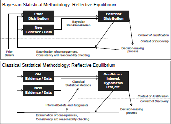
For both schools of statistics, problems to be solved are not isolated textbook cases, but rather originate in informal, non-statistical beliefs and inputs. And in both cases, the finished statistical analysis is not immediately entered into a blank to be graded, but must provide output couched in concepts and vocabulary that integrated into existing decision­making processes.

With that in mind, here are some quick pros and cons of Bayesianism statistics. Of course which approach is best depends on the exact problem and circumstance in question, but some generalizations seem useful. First the pros:

• It makes sense - Bayesianism is based on a consistent and beautiful idealization of rationality. When Bayesian priors are available and the computation is feasible, Bayesian analyses may be the obvious choice.
• Coherence - Unlike classical statistics which can seem like a grab bag of random ideas, Bayesianism techniques follow from only a few core ideas.
• Documentation - Bayesian analyses typically formalize more of their assumptions, instead of smuggling them in like classical statistics. This allows more information to be communicated in work products.
• Intuitive outputs - Bayesian analyses typically produce posterior probabilities for theories (or Bayes factors comparing two theories), and credible intervals or posterior distributions for parameters. These are much more useful and less error-prone than their counterparts, classical hypothesis testing and confidence intervals.
• Decision theory - Bayesianism shares a tight connection to decision theory. Most insurance decisions are not made formally, but decision theory may occasionally be useful.

Now for some general cons of Bayesian statistics:

• Priors can be difficult - As mentioned above, people do not actually have prior prob­ability functions in their heads. For many problems, it can be very hard to construct an appropriate and practical prior.
• It is subjective and nitpickable - This is the flipside of self-documenting above. Some­times it is not a good idea to expose certain assumptions and the arbitrariness of certain decisions.
• Computationally difficult - Even relatively simple Bayesian problems may require MCMC methods. Convenient computation is extremely important; the less time spent computing, the more time can be spent doing additional analyses, doing data valida­tion and exploration, etc.
• Unwieldy outputs - A full posterior distribution may be conceptually intuitive and may contain all relevant information, but may be harder to process than the classi­cal equivalent. For instance, compare the posteriors from Bayesian regression to the simple point estimates and covariance matricies from classical regression.
• Unfamiliar language - Apart from their intrinsic merit, many people may be more familiar with classical concepts. For instance, when talking to someone who frequently does Kolmogorov-Smirnov tests, simply communicating the K-S statistic may be the best option.

3.6 Conclusion

The foundations of Bayesianism are based on the idea of subjective probabilities. Although considered philosophically problematic by frequentists, they are both mathematically solid and lead to beautiful and productive theories of statistics, game theory and decision theory.

Conditionalization is core to Bayesian statistics. When you learn evidence e, you should condition on it by moving from your prior subjective probability distribution $\mathbb{P}(\cdot )$ to the posterior distribution $\mathbb{P}\left(\cdot |e\right).$

Despite the simple notation, $\mathbb{P}\left(\cdot |e\right).$ can be hard to compute in practice because it involves calculating the integral $\int p\left(e|\varphi \right)p\left(\varphi \right)d\varphi .$ In the case of Bayesian conjugates, there is an exact solution, but typically this integral must be sidestepped or approximated. The most popular approach is to use MCMC methods to sample from $\mathbb{P}\left(\cdot |e\right)$ rather than computing it directly. There are a variety of R packages and MCMC engines to help with this.

Bayesian statistics is based on an elegant theory of rationality and can be applied to almost any statistical problem. However, it is not always the best choice in practice. Solving actuarial problems involves producing work products, not posterior distributions. Bayesian statistics provides actuaries with a rich and useful set of tools, but techniques from classical statistics, machine learning or other fields will fit certain situations better.

3.7 Exercises

3.1. Consider a simple mixture model, with two components, $p.N\left({\mu }_{1,}1\right)+\left[1-p\right].$ where the probability μ is known. Assume further that μ < 0.5 to make sure that the model is identifiable (and ${\mu }_1$ cannot be confused with m2). We do have a sample {x1,..., xn}. Assume independent priors $N\left(a,1/b\right)$ on both ${\mu }_1\text{ and }{\mu }_2$ .

Write the code of the following algorithm (so-called Gibbs sampler for mean mixtures), function of vector x (the observations) and of vector c(a,b), the fixed hyper-parameters of the prior distribution. To initialize, chose ${\mu }_{1,0}\text{ and }{\mu }_{2,0}$ Then, at iteration $k\left(\text{with }k\ge 1\right),$

1. (a) Generate ϴi, which will allocate i to one group, either 1 or 2, with probabilities
   $\{\begin{array}{c}\mathbb{P}\left({\Theta }_i=1\right)\alpha p\cdot \exp \left(-\frac{1}{2}{\left[x_i-{\mu }_{1,k-1}\right]}^2\right)\\ \mathbb{P}\left({\Theta }_i=2\right)\alpha \left[1-p\right]\cdot \exp \left(-\frac{1}{2}{\left[x_i-{\mu }_{2,k-1}\right]}^2\right).\end{array}$
2. (b) Compute ${\beta }_k=\sum _{i=1}^{n}1\left({\Theta }_i=1\right),$ the number of observations in class 1, the total sum for observations in class 1 ${\alpha }_{1,k}=\sum _{i=1}^{n}1\left({\Theta }_i=1\right)\cdot x_i$ and the total sum for observations in class 2 ${\alpha }_{2,k}=\sum _{i=1}^{n}1\left({\Theta }_i=2\right)\cdot x_i$
3. (c)Generate ${\mu }_{1,k}$ from $N$ ${\mu }_{1,k}\text{ from }N\left(\frac{ab+{\alpha }_{1,k}{\beta }_k}{b+{\beta }_k},\frac{1}{b+{\beta }_k}\right).$
4. (d)Generate ${\mu }_{2,k}$ from N${\mu }_{2,k}\text{ from }N\left(\frac{ab+{\alpha }_{2,k}(n-{\beta }_k)}{b+n-{\beta }_k},\frac{1}{b+n-{\beta }_k}\right).$