
Chapter 8
Forms of Neural Network Learning
8.1 Using Multilayer Neural Networks for Recognition
Multilayer neural networks covered in detail in earlier chapters can handle many tasks. Nevertheless, if we want to analyze their properties and the way they work, the most appropriate area is probably image recognition in which a neural network (or other type of learning machine) classifies images into certain classes. The analyzed objects may vary widely, from digital camera images to scanned or grabbed analog images. We present a comparison of digital and analog images in Figure 8.1 to help explain this point. Each neuron of the hidden layer receives three weights for neurons 1.1 and 1.2; each neuron of the output layer receives three weights for neurons 2.1 and 2.2.

This book is about neural networks and not about images. Hence, we will not delve deeply into the theories of image recognition. However, the challenge of having a machine recognize images started a new field of computer science. The first neural network built by Frank Rosenblatt (Figure 8.2) was used to recognize images and was thus called a perceptron. While of poor quality, the figure is a relic of an early and outstanding achievement in the area of computer outputs.

The meaning of image has become so general that neural networks are used now for recognizing samples of sound signals (spoken commands), seismic or other geophysical signals, symptoms of patients to be diagnosed, scores of loan applicants, and other tasks. All these tasks involve image recognition although the images in the areas cited are in fact acoustic, geophysical, diagnostic, and economic.
A neural network used for image recognition usually needs several inputs supplied with signals representing features of the objects to be recognized. These may, for example, be coefficients describing the shape of a machine part or liver tissue texture. We often use many inputs to show a neural network all the features of an object so that the network learns how to recognize the object correctly. However, the number of image features is far fewer than the number of image elements (pixels). If you supply a network with a raw digital image, the number of its inputs can reach millions. That is why we rarely use neural networks to analyze raw images. The networks usually “see” the features of an image extracted by other programs outside the network. This image preparation is sometimes called “preprocessing.”
A neural network used for recognition usually generates several outputs as well. Generally speaking, each output is assigned to a specific class. For example an optical character recognition (OCR) system may use over 60 outputs, each assigned to a certain character (e.g., the first output neuron indicates A, the second neuron denotes B, etc.). We discussed this in Chapter 2. Figures 2.30, 2.31, and 2.33 depict the possible output signals of a network used for recognition.
At least one hidden layer or neurons is generally sited between the input and output layers of a network. We will now study the hidden layer in more detail. A hidden layer may contain a few or many neurons. After analyzing briefly the functioning of neural networks, we usually think that more neurons in a hidden layer constitute a smarter network. However, we will see that a network with great intelligence may also be disobedient.
8.2 Implementing a Simple Neural Network for Recognition
We are now going to build a sample network with two inputs. In reality, it is not possible to recognize an object based on only two features. For this reason neural networks are most commonly used to analyze multidimensional data whose outputs require more than two inputs. However, using two inputs in our example has a significant advantage: each recognized object may be represented as a point on a plane. The first and the second coordinates of the point indicate the values of the first and second features, respectively.
We encountered a similar situation in Chapter 6 (Section 6.4) where we imagined a brain of a hypothetical animal as a two-dimensional input space with two primitive receptors—eyes and ears. The stronger the signal captured by the eyes, the more to the right is the point on the plane; the stronger the sound, the higher the point is on the plane. Figure 6.8 will be useful for explaining this material.
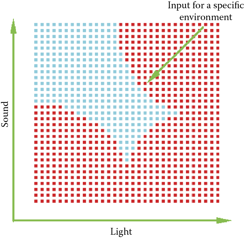
Every image shown to the network (each environment of the animal) may be shown as a point on an axis or as a pixel on a screen. The coordinates correspond to the features of the environment (Figure 8.3). We will use a screen of a fixed size so we should start by limiting the values of our features. In the example considered here, both features of the analyzed image will take values from –5 to +5. You will have to remember that scale when formulating tasks for the network.
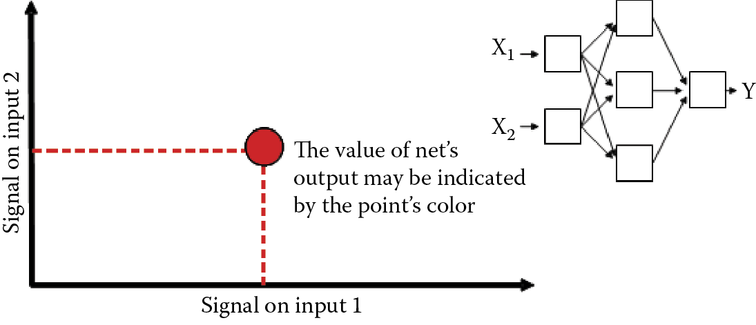
Each network has an output we will use to observe its behavior. Our example will always generate one output. We have already interpreted its meaning in Figure 6.8.
To review, the animal may react to a presented situation with a positive or negative attitude indicated by the intense red or blue color, respectively. We will place our animal in various environments by supplying the network with sets of input signals that correspond to positions of the animal as it senses different features. You will be able to prepare a map of places where the animal is comfortable and where it is not. The map should be built of separate points because it will be created by the program we are going to run (Figure 8.4). To improve the appearance of our maps, we will “smooth” them (Figure 8.5).

As the network grows, we will more often observe intermediate states: partial disgust (light blue), neutrality (light green), and partial applause (yellow turning to light red); see Figure 8.6. The fact that the network has only one output will make its workings easy to understand. By switching on a pixel corresponding to a certain input vector, you will see whether the point is accepted (red) or rejected (blue) by the network. Of course, the data describing these points will have to be prepared by the program; this will be covered later.

You will see maps like these during network training. They will change as the network dislikes an item it approved earlier or accepts something it already rejected. It is interesting to watch how initial confusion turns into a working hypothesis and then crystallizes into absolute certainty. It is not easy to illustrate these phenomena so clearly for a multiple-output network, but the exercise is necessary because real-world systems usually generate many outputs.
Using only one output in our example has another advantage: you don’t have to decide whether the better network is one that classifies a signal into several classes at a time with the same confidence or a network that generates all weak responses among which the strongest is the correct one. Multiple-output networks may create other problems and thus it is difficult to judge performance of a network based on its reaction to unseen situations (ability to generalize its knowledge). The result from a single-output network is always clear.
8.3 Selecting Network Structure for Experiments
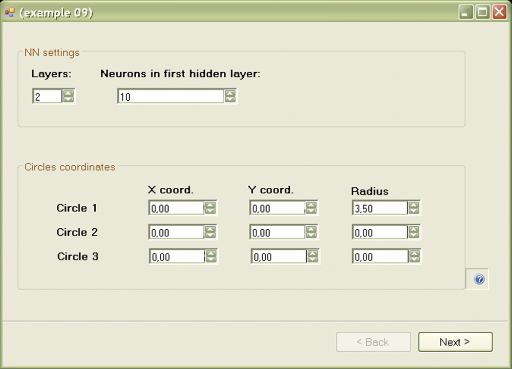
The Example 09 program allows you to experiment with network structures. At opening, the program shows a panel for defining the structure of the network to be tested (Figure 8.7). The program will suggest default parameters that may be changed and we will do that as an exercise.

The network you are going to teach and analyze will have a 2 - xxx - 1 structure. The successive numbers stand for two inputs, a number to be modified in the course of teaching (xxx) and one output. To define a specific network, you will only have to specify the number and the order of hidden neurons (how many hidden layers to create).
You will be able to define the number of neurons in each layer of the network, depending on how many layers you choose in the Layers field. When specifying numbers of layers, remember that the only layers that count contain neurons that can learn. That is why the output layer counts, although it contains only one neuron and the two input neurons that accept only input signals do not count. Thus if you choose a one-layer network, you will get 2 - 1 and be unable to specify the number of hidden neurons as this number is fixed by the network architecture.
If you choose a two-layer network, the structure will be 2 - x - 1 and the Neurons field will appear in the hidden layer in which you can specify the number of hidden neurons (Figure 8.8). Finally, if you choose a three-layer network (or leave the default settings unchanged), the resulting architecture will be 2 - x - y - 1 and will have to set the number of neurons in both hidden layers (the Neurons field in the first hidden layer and also in the second hidden layer).

Our program cannot simulate networks of more than three layers. You may try to change this limitation by “playing” with the source code. We chose to limit the number of layers because the program works slowly for large networks. You will see that a few hundred training steps (not many for a learning process) will take time even with a fast computer.
8.4 Preparing Recognition Tasks
After choosing the size of the network, and if necessary, the numbers of neurons in all its layers, we may proceed to the most interesting step: preparing the task to be solved. As you know, the concept of recognition is that a network should react positively to (“recognize”) certain combinations of input signals (images) and react negatively (“reject”) other combinations. The training set for the Example 09 program is shown in Figure 8.9. It consists of a certain number of points on a plane, each of which has two coordinates so that we know where to put a point on the screen and we know the network will produce a positive (red [darker]) or negative (blue [lighter]) response.

The user decides where to put blue and red points indicating acceptance and rejection. You could attempt this experiment manually using sets of three numbers (two inputs and one output) but the final image or preference map would be difficult to generate and interpret. For that reason, we designed Example 09 to generate examples automatically. The user’s task is simply to show the network the positive and negative areas. Again, the system made the decisions. You could certainly specify the shapes of these areas but that would require including a complex graphical editor in the program that would be hard to use.
We sought a middle-of-the-road solution. The areas of positive decision (fragments of input space to which the network should respond positively by red points on the plot) will belong to three circles. This is a large constraint, but also a fast and comfortable way of preparing tasks. You will be able to devise interesting problems for the network, by combining the three circles of any size at any position.
You may set the coordinates of these three circles in the same window (the first one that appears after the program starts) in which you defined the architecture (Figure 8.10) of the network. First coordinates (x and y) define the center of the circle and the third coordinate defines its radius. You may set values for the three circles independently. You are free to choose these parameters, but as noted earlier, only the part of the plane for which both coordinates are in the range –5 to 5 is used in the recognition process. A circle with parameters 0, 0, 3 positively would be a reasonable area for placing the points; however, a circle with parameters 10, 10, 3 may not be so, and hence, not useful in our experiments.
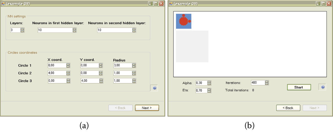
(a) Defining network structure and regions for recognition. (b) Map of regions to which the network should react with a positive or negative answer after training.
After setting the parameters of the task to be solved by the network, you may see the results of your choice in the next panel where the network is simulated. You reach this panel by pressing the Next button at the bottom of the window (Figure 8.10). The results of your decisions are shown as a map of positive and negative response areas. This allows you to check easily whether your expectations of learning were met. If you choose not to specify a task, you may always return to the previous panel by pressing the Back button. This will allow you to modify the center coordinates and sizes of the circles.
Training will start when a random point for which the class will be decided according to your map is chosen, then a set of two input coordinates and the desired class will be supplied to the network as an example from the training set. This procedure will be repeated many times.
We must note one detail that is easy to miss. If you define the decision areas so that most of the decision plane is positive (red), the network will usually chose these examples during training and will rarely utilize the points generating negative answers. Thus it will learn negative reactions slowly. The impact on positive reactions will occur if a network is trained with excessive negative (blue) examples. Approximately the same numbers of red and blue training points were included in our training set to maintain a network’s ability to handle both negative and positive signals efficiently.
After specifying the task as a map that is well balanced and meets your needs, you can start training the network by pressing the Start button (Figure 8.10). You will see the network’s assignments of random weights to all its neurons. Usually this initial distribution has no relation to the task you defined. How can a network possibly know what result you want before it is trained? It is helpful to compare this initial map with the map of the task.
Training success depends on how similar these two maps are at the beginning. If they look alike, the network will learn quickly and effectively. If the maps differ significantly, the network will learn slowly. Little progress will be seen initially because the network will have to utilize its inborn intelligence to start improving its functioning (Figure 8.11).

The structure of the figure displayed requires some explanation. The small rectangles filled with color spots that appear during the simulation represent the “consciousness” of the network during each training state. As you know, each point inside the rectangle represents two features (corresponding to coordinates of the point) that serve as input signals. The color of each point indicates the network’s answer to the input.
Consider the first two rectangles in the upper left corner of the figure. The first one shows what you want to teach the network. Following the steps described in the preceding section, you set conditions to be accepted or rejected by your “animal” and they are shown on the map of desired reactions. The second rectangle in the upper row shows the network’s natural predispositions. Each experiment may involve different initial parameters set randomly. Thus, the network’s behavior is unpredictable.
The remaining diagrams correspond to the subsequent stages of training. They are drawn as rectangles in Figure 8.11 and may be shown as different time steps. The user determines (using the Iterations field) the number of steps of training before showing the results. The Iterations field includes an additional read-only feature called Total Iterations that shows the total number of training steps already performed.
Before performing the number of steps set at the preceding state or specified by you, you may change the values of the training coefficient (alpha) and momentum coefficient (eta) parameters in the corresponding fields shown on the screen. You may set them to any values, but we advise you to retain the defaults during training. After you learn the components of the training process, you may want to experiment with the parameters to see how they affect the results.
8.5 Observation of Learning
The Example 09 program allows you to investigate many aspects of learning by neural networks. We spent many hours devising tasks for networks and analyzing combinations of training parameters to make the program experiments interesting and enlightening.
Learning processes in living organisms, particularly neural mechanisms that determine and control learning, have always been key interests of biological scientists. Through the years they studied learning in humans and animals to learn the basic components of the process. Their findings based on behavior have revolutionized education and training methods but we still do not understand fully the mechanisms behind the processes.
Thousands of neurophysiological and biochemical experiments conducted to dissect learning processes yielded less than satisfactory results. Fortunately, new methods have revealed some aspects of neural system functioning. Many of these methods use artificial neural networks to simulate learning processes and utilize programs like Example 09.
As you remember, training a neural network involves submitting examples of input signals (chosen randomly from the training dataset) to its inputs and motivating the network to produce an output according to the map of preferred behaviors. This scenario may be adapted to the earlier example of an animal with two senses (sight and hearing).
We place the animal in various conditions that allow it to sense random (but known) signals. The animal (or neural network) reacts according to its current knowledge. It accepts some conditions and rejects others. The teacher (training computer) that has a map of preferred reactions supplies the network with the desired output signal, in essence telling the network to “like this and dislike that.”
You may watch the training process on your screen. The large square in the lower left corner of the example screen illustrates points corresponding to the input signals presented to the network. As you can see, they are randomly chosen from the entire area of the square. Each point is marked in red or blue based on the teacher’s suggestions. The network uses these instructions and corrects its errors by adjusting its parameters (synaptic weights). The adjustment is performed according to the backpropagation algorithm presented earlier.
The training pauses periodically and the network is examined. The network should generate answers for all the input points. The results are presented as maps of color points arranged as consecutive squares from left to right and from the upper to lower rows of the image produced by Example 09. After each such pause, the user determines the number of steps until the next examination.
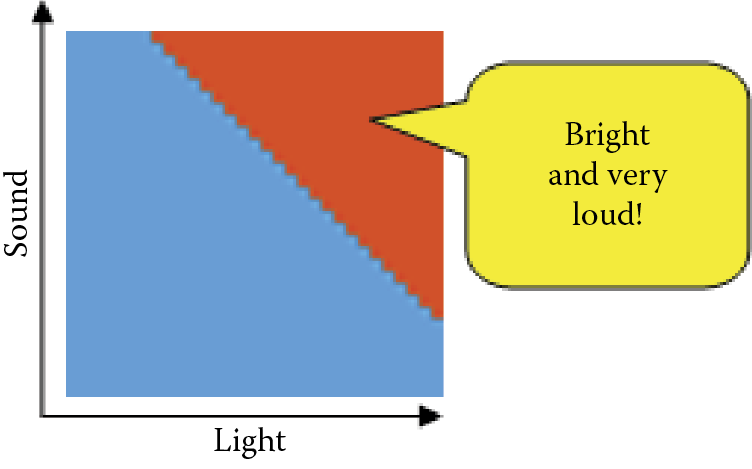
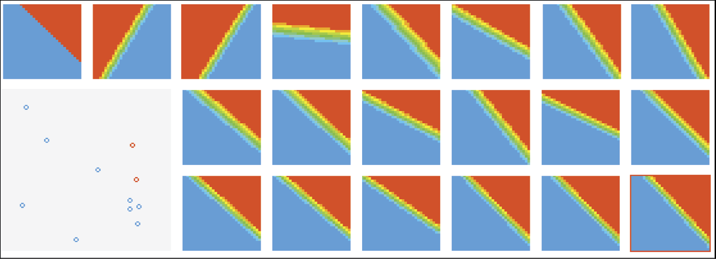
We will begin by demonstrating the ways neural networks learn using an example of a one-layer network denoted 2, 1. The network’s task is simple: divide all possible input data into approved and rejected regions using an almost straight line. To define this problem, the following coordinates of three circles were defined in the program:
100, 100, 140
0, 0, 0
0, 0, 0
We defined a map of preferred behaviors that is simple and easy to interpret (Figure 8.12). It indicates our animal should seek a bright and loud environment.
As you know, the Example 09 program examines the natural (inborn) preferences of the network at the start. The second square on the screen (Figure 8.13) should be regarded as a complete result of testing the animal before it starts to learn. The program places the animal in every possible environment (checks all points inside the square) and waits for a reaction. Each point is drawn red if a reaction was positive or blue if negative. The color scale is continuous to illustrate all the reactions between the two extreme stages. As we can see, our animal initially likes dark and silent places but it tolerates some light. Generally the more sound it hears, the more light it accepts.

The network you will train on your computer will have a different map of initial preferences because they are random. Because the network’s state desired by the teacher and the actual state are very different, as occurs in most experiments, intensive training must take place. You proceed by specifying the number of training steps to perform before the program pauses to show the decision map. We suggest you watch the training effects in small networks fairly often, say, every 10 steps. For larger networks of several layers and many hidden neurons, much more training is needed to yield results. For now it is sufficient to specify the lengths of subsequent training epochs, then watch, compare, and learn. That is the best way to analyze the workings of neural networks; it is more effective than studying loads of scientific books and articles.
We now suggest you analyze some training stages that we observed while preparing examples for this book, although your computer may generate somewhat different images. The rectangle we obtained after the first stage of training (Figure 8.14) shows an image similar to that of a “newborn” network. This means that despite intensive training, the network is holding onto its original beliefs. This attachment is typical for neural networks. The same dynamic appears when people and animals learn.

The next stage of training adds another square to the figure and shows intermediate training. The network starts to change its behavior but it is far from the final solution. The boundary between the positive and negative areas is almost horizontal (Figure 8.15). The network “thinks” it knows the teacher’s intentions but more adjustments are needed. After another segment of training, the network’s behavior more closely resembles the desired one, but the position of the decision boundary is not ideal yet (Figure 8.16).


You may consider this performance outstanding, especially based on the short time it took to achieve such a result. Generally we should stop training at this stage. However, for exploration purposes, we continued training the network, assuming that our strict teacher aims for absolute perfection and compels the network to adjust even very minor mistakes. The only effect of the next stage of training is a sudden crisis. The network performance deteriorates and the decision boundary position is worse than it was earlier (Figure 8.17).

A long time and many training steps were required for the network to recover and achieve the accuracy level imposed by the teacher. This effect is worth noticing. At this training stage, the network’s knowledge is not yet stable. Excessive teaching rigor at this state is usually damaging and in extreme cases can lead to a complete breakdown of the learning network. The process of learning this simple task after 12 training steps is presented in Figure 8.18.
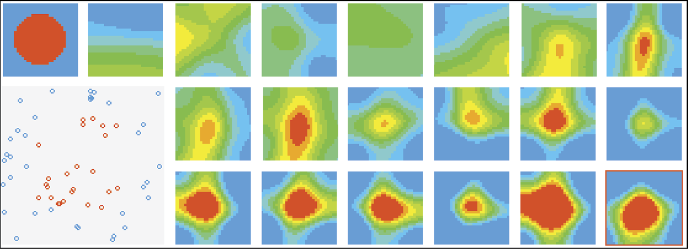
We will interrupt the training sequence and return to the screen on which we set new parameters for the problem to be solved. After specifying the same network structure (one-layer network), we will formulate a more difficult task. We want our animal to be enthusiastic about “the golden mean” which is an Aristotelian philosophy that is a desirable mean between two extremes: excess and deficiency. Thus, it needs to discard all the extremes and feel comfortable only in a specific environment. It is easy to do this by defining only one circle to be learned, as follows:
0, 0, 3, 5
We shrink the other two circles to zeros:
0, 0, 0
0, 0, 0
The scheme of ideal network behavior is presented in Figure 8.19.

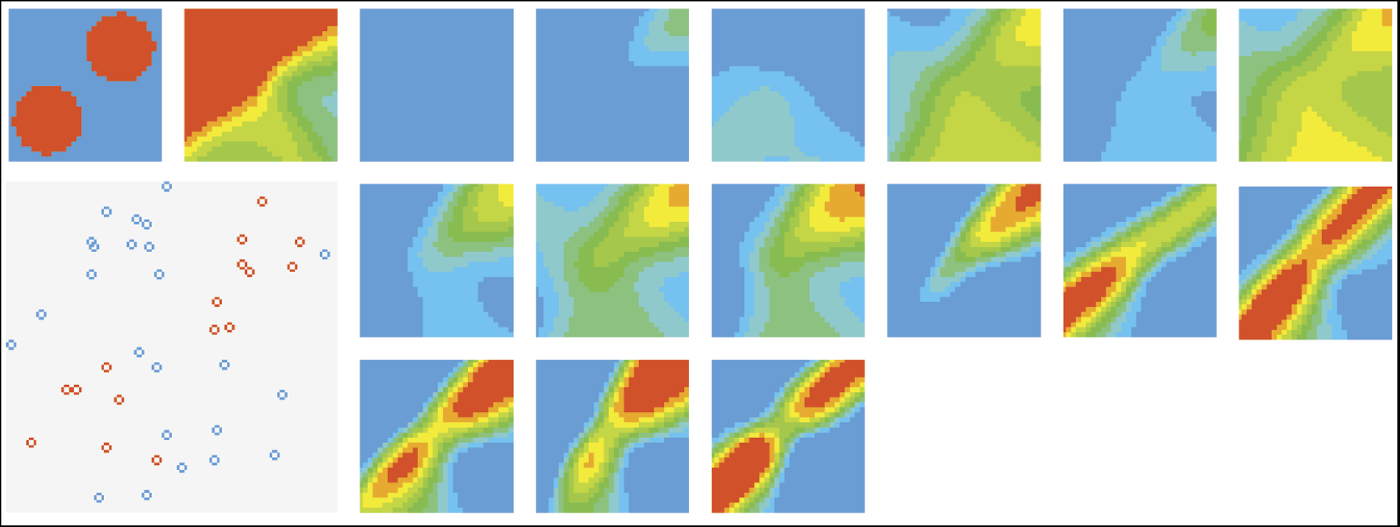
Observe the learning process in Figure 8.20 (prepared in the same way as Figure 8.18). We can see that the network struggles and continuously changes its behavior in attempts to avoid the penalties imposed by the teacher—without success. Whatever parameters are chosen for a network and however the decision boundary between positive and negative reactions is set, the network will always fall into the trap of accepting a region of extreme conditions.

Subsequent figures show that the animal tries to hide in the darkness, accepting the examples with small amounts of light. This behavior will be punished by the teacher in the next steps of training. Before we interrupted the experiment, the animal formulated another incorrect hypothesis. It started to avoid the regions of silence, thinking that the clue to success was noise. This action was also incorrect.
The reason for these failures is simple: the modeled neural network was too primitive to learn a complex behavior such as choosing the golden mean. The network we used in our experiment was capable of understanding only one method of input signal selection—linear discrimination—which was too simple and primitive for the second problem.
Therefore, the next experiment will engage a larger and more complex network for the same task. When setting the structure, we may specify the parameters as shown in Figure 8.21. After we set more than one layer in a network, the program asked for the number of neurons. In brief, more layers require more answers and provide greater intellectual potential. Such a network can better use its inborn intelligence.
We can see how it learns. Its initial distribution of color areas shown in Figure 8.22 indicates that the network is initially enthusiastic about all values. The modeled animal feels comfortable in most situations although it prefers dark and quiet corners.

The first training steps show the network that the world is not always perfect. The network reacts in a typical way. At the start, it cultivates its initial prejudices. It is less positive about dark places after the first stage of training, but still far from the final result (Figure 8.23). Further training leads our animal through a series of disappointments. It receives punishment for being too trusting and enthusiastic. It formulates a more suspicious attitude toward the untrustworthy world. Its initial enthusiasm and favorable view diminishes to a slight fondness for quiet and sunny places (small yellow dot at the bottom right of the last square on Figure 8.24).


However, this attitude also meets the teacher’s disapproval. After the next training stage, the animal (network) becomes completely stagnant and rejects everything (Figure 8.25). This state of discouragement and breakdown is typical for neural networks in training and usually precedes attempts to construct a positive representation of the knowledge desired by the teacher.

In fact our network tries to create an image like Figure 8.26. Only a few positive examples shown by the teacher are enough for the network to revert to a phase of enthusiasm and optimism in which it approves all the environments except those that are very loud and dark. Total darkness and intensive light reduce its tolerance for loudness. Of course, the next training stage must suppress this enthusiasm so the network returns to the states of rejection and frustration, retaining only traces of positive memories that did not lead to punishment. In the next stage, the small positive reaction will become the seed of a correct hypothesis (red [dark] spot near the middle of the volatility region in Figure 8.27).


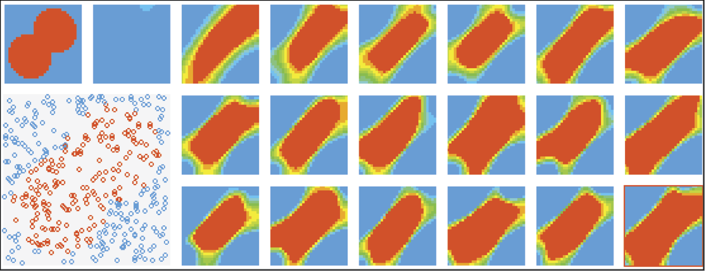
After that, training is only about controlling another rush of enthusiasm and reducing the area of positive reactions to a reasonable size. When we interrupted training after 15 stages, the network appropriately followed the teacher in this signal classification task so that further improvement of its performance was not necessary (Figure 8.28). As we can see, the system with larger and more efficient “brain” (more than ten times more neurons and more powerful connections between them) was capable of learning behaviors the smaller system could not manage to learn.

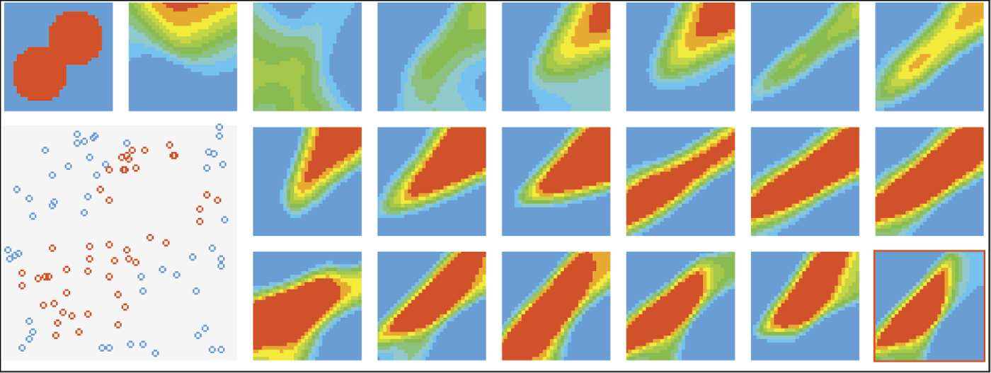
Another interesting experiment is presented in Figure 8.29. It illustrates how the same ability (of reasoning that the teacher wants acceptance of medium light and sound conditions and rejection of the extremes) is learned by another network with the same structure as the one analyzed in Figure 8.28. In the training process depicted in Figure 8.29, the network is somewhat melancholic at the start of training even though it has the same structure as the network in Figure 8.28. The figure is dominated by cool green and blue colors indicating apathy or dislike.
Initial training makes it a little more interested in “disco” conditions (yellow spot in the rectangle illustrating the first training stage). Several consecutive failures throw the network into an area of rejection. At the fourth training stage, the network tries to put forward a hypothesis that the teacher wants it to approve bright and medium loud places. At the next stage, the network guesses the average conditions to be accepted. As training continues, the hypothesis grows stronger and clearer as shown by the red (dark) dot indicating complete acceptance.
With each training step, the dot’s shape matches more exactly the acceptance area set by the teacher. Green and yellow areas of confusion and uncertainty are replaced by more exact divisions into like and dislike conditions. Finally the melancholic network learns to act exactly the same way as the enthusiastic network. This proves that built-in predispositions are not controlling. Strong and focused training always achieves its goal but methods of reaching it vary based on starting points.
You may perform many different experiments using our program. Figures 8.30, 8.31, and 8.32 show a few of them. You will benefit from analyzing these figures, reconstructing them on your computer, and conducting your own experiments to study training variations and results.
Compare Figure 8.30, Figure 8.31, and Figure 8.32 with Figure 8.20. You can see how the behavior of an intellectually well-equipped network differs from the behavior of a simple network that cannot learn more sophisticated rules. Note that the neural “simpleton” could not learn simple behaviors but its reactions were very strong and categorical. The world is only black or white for this network. An object is absolutely good or definitely wrong. If the network’s experience failed to conform to these extremes, it generated another opinion—far more rigid and usually incorrect.

The networks with more intellectual power were able to model more subtle divisions. However, they took more time to reach their goals and remained in inactive states (hesitation, breakdown, and indecision) longer. Despite these downsides, these neurotic, hesitating, excessively intelligent individuals reached the goal of understanding the teacher’s rules and adjusting to them, while the tough moron circled and failed to reach a rational conclusion.
Notice how many interesting and diverse behaviors of neural networks we observed with one simple program. The computer running it did not resemble a dull and limited machine or perform monotonously and repeatedly. On the contrary, it demonstrated some individual characteristics, mood changes, and a variety of talents. Does that remind you of anything?
8.6 Additional Observations
We could end this now, leaving you to use the program to discover more interesting aspects of training, but we will suggest some sample shapes worth investigating before you pursue real-life projects. Our experiments showed that interesting training results may arise from using a snowman made of three circles:
0, 0, 3
4, 0, 1
0, 4, 1
The task is complicated enough so that the network must work hard to discover the actual rule of recognition. The network for this task should have three layers and high numbers of neurons in its hidden layers (17 neurons in the first hidden layer and 5 in the second). The task is also sufficiently compact to be displayed on the screen so the results are easy to observe. We will not show you the results for these examples because you may want to discover the properties of neural networks and their sensitivities to some parameters that affect training.
As you know, you may specify training parameters that influence the speed of the program before it executes the number of training steps you select. The first (alpha) parameter is the learning rate. The greater the learning rate, the more intense the training process. Alpha sometimes yields good results or it may lessen them. This is another area for program exploration. The second parameter (eta) is momentum. It makes learning conservative: the network does not forget the previous directions of weight changes while performing a current training step. Again, higher eta values may help learning or impede it.
The learning rate and momentum coefficients are always accessible in the program window of Example 09 and they may be changed during training to allow a user to observe interesting results. They may be modified only once before learning starts. You will see that training accelerates with higher alpha values. Figure 8.33 presents the training process for a task with standard values and Figure 8.34 shows training at higher alpha level.

An overly high alpha rate, however, is not effective. It can trigger instability as illustrated in Figure 8.35. The way to suppress the oscillations that result from too high a learning rate is to increase the eta (momentum) coefficient. You may wish to analyze the effect of changing momentum on training and demonstrate its stabilizing power when training goes out of control.

Excessive learning rate produces oscillations. Network approaches desired solution, then changes direction.
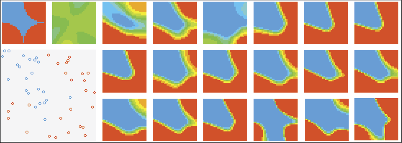
Another possible area of interesting research is the dependence of behavior on network structure. To analyze that, you must choose a very difficult problem to be learned. A good one is presented in Figure 8.4 and Figure 8.5. The difficulty is the need to fit the blue area defining negative into tight bays (Figure 8.36). Very precise parameters must be chosen to fit the slots; this is a large challenge for a network.

A three-layer network can distinguish all the subtle parts of a problem (Figure 8.37), although it is sometimes difficult to maintain training stability. This type of network, even when it is close to a solution, may abandon it due to backpropagation of errors and search for a solution in an area where a correct solution cannot be found (Figure 8.38). You may use your imagination and freely define the regions where a network should react positively and negatively. You may run tens of experiments and obtain hundreds of observations. Just remember that training a large network may take long time, especially in the initial stages. You will need a very fast computer or a lot of patience. We suggest that patience is cheaper.

Questions and Self-Study Tasks
1. Does image recognition refer only to visual images (e.g., from a digital camera) or does the phrase have a wider meaning?
2. How do we input image data (and information about objects to be recognized) into a classifying neural network?
3. How do neural classifiers usually present the outcomes of their work. How do they demonstrate what they recognized? What consequences does the presentation method have on the usual structure of the output layer?
4. Use the observations from this chapter for training networks for several problems with theoretical information from Chapter 6 explaining how multilayer networks with different numbers of layers work. Notice the greater capabilities of the networks presented in this chapter resulting from the use of neurons that can produce continuous output signals instead of only 0 and 1 values.
5. Think about the relationship of the number of hidden neurons in a complex multilayer network and the number of separate areas in the input space that allow a network to learn to make 0-or-1 decisions.
6. Figure 8.39 illustrates the relation between numbers of hidden neurons and network efficiency in performing learned tasks. The left side of the plot is easy to interpret: a network with a small number of neurons is not “intelligent” enough to solve the problem and adding neurons improves its performance. How should we interpret the concept (proven many times in neural networks) that too many hidden neurons will deteriorate the performance of a network?

7. Learning rate measures the intensity of weight adjustments applied to a network after detecting a faulty operation. The informal interpretation of learning rate is that high values represent a strict and demanding teacher and small values correspond to a gentle and tolerant one. Explain why the best training results are observed for moderate values of learning rate (neither too small nor too high). Try to confirm your explanation by experimenting with our program. Plot learning rate versus training performance after a set number of epochs (after 500, 1000, and 5000 steps).
8. Many training methods in which the learning rate is not constant throughout the process are known. Under what conditions should the learning rate be increased and when should it be reduced?
9. Some training theories suggest that the learning rate should be small at the beginning when network makes a lot of mistakes. If we apply strong weight changes in response to the errors, the network would experience “convulsions,” avoiding some mistakes and making new ones. Early in training, a network needs a gentle and mild teacher. As it gains more knowledge, the learning rate can be increased because the network will make fewer and less serious mistakes. At the end of training after the network acquires a lot of knowledge, a slower learning rate is advisable, so that incidental mistakes (caused by a few challenges in the training set) do not spoil the result since improvement of one area produces weakening in other areas. Design experiments to confirm or negate this theory.
10. We can compensate for the effects of a too-large learning rate value that can risk the stability of training by increasing the momentum coefficient that measures the conservatism of training. Design and conduct some experiments to generate a plot showing what minimal values of momentum are needed for different values of learning rate to guarantee fast and stable training.
11. Advanced exercise: Modify our program so that it can define the regions for different classes (areas where the animal should feel comfortable and uncomfortable) with the use of a graphical editor. Use this tool to build a network that will learn a very difficult problem, in which these regions are defined as two spirals (Figure 8.40).

12. Advanced exercise: Design and make a model of an animal with more receptors (senses to observe features of the environment) and capable of more complex actions (moving through the environment to seek conditions it likes or search for food. Designing and observing a neural network as the brain of an animal may be a fascinating intellectual adventure.