
CHAPTER 1
What is computation?
We need to do away with the myth that computer science is about computers. Computer science is no more about computers than astronomy is about telescopes, biology is about microscopes or chemistry is about beakers and test tubes. Science is not about tools, it is about how we use them and what we find out when we do.
Michael R. Fellows and Ian Parberry
Computing Research News (1993)
COMPUTERS are the most powerful tools ever invented, but not because of their versatility and speed, per se. Computers are powerful because they empower us to innovate and make unprecedented discoveries.
A computer is a machine that carries out a computation, a sequence of simple steps that transforms some initial information, an input, into some desired result, the output. Computer scientists harness the power of computers to solve complex problems by designing solutions that can be expressed as computations. The output of a computation might be a more efficient route for a spacecraft, a more effective protocol to control an epidemic, or a secret message hidden in a digital photograph.
Computer science has always been interdisciplinary, as computational problems arise in virtually every domain imaginable. Social scientists use computational models to better understand social networks, epidemics, population dynamics, markets, and auctions. Scholars working in the digital humanities use computational tools to curate and analyze classic literature. Artists are increasingly incorporating digital technologies into their compositions and performances. Computational scientists work in areas related to climate prediction, genomics, particle physics, neuroscience, and drug discovery.
In this book, we will explore the fundamental problem solving techniques of computer science, and discover how they can be used to model and solve a variety of interdisciplinary problems. In this first chapter, we will provide an orientation and lay out the context in which to place the rest of the book. We will further develop all of these ideas throughout, so don’t worry if they are not all crystal clear at first.
1.1 PROBLEMS AND ABSTRACTION
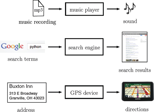
Every useful computation solves a problem of some sort. A problem is fundamentally defined by the relationship between its input and its output, as illustrated in Figure 1.1. For each problem, we have an input entering on the left and a corresponding output exiting on the right. In between, a computation transforms the input into a correct output. When you listen to a song, the music player performs a computation to convert the digital music file (input) into a sound pattern (output). When you submit a web search request (input), your computer, and many others across the Internet, perform computations to get you results (outputs). And when you use GPS navigation, a device computes directions (output) based on your current position, your destination, and its stored maps (inputs).
Inputs and outputs are probably also familiar to you from high school algebra. When you were given an expression like
y = 18x + 31
or
f(x) = 18x + 31,
you may have thought about the variable x as a representation of the input and y, or f(x), as a representation of the output. In this example, when the input is x = 2, the output is y = 67, or f(x) = 67. The arithmetic that turns x into y is a very simple (and boring) example of a computation.
Reflection 1.1 What kinds of problems are you interested in? What are their inputs and outputs? Are the inputs and outputs, as you have defined them, sufficient to define the problem completely?
To use the technologies illustrated in Figure 1.1 you do not need to understand how the underlying computation transforms the input to the output; we can think of the computation as a “black box” and still use the technology effectively. We call this idea functional abstraction, a very important concept that we often take for granted. Put simply,
A functional abstraction describes how to use a tool or technology without necessarily providing any knowledge about how it works.
We exist in a world of abstractions; we could not function without them. We even think about our own bodies in terms of abstractions. Move your fingers. Did you need to understand how your brain triggered your nervous and musculoskeletal systems to make that happen? As far as most of us are concerned, a car is also an abstraction. To drive a car, do you need to know how turning the steering wheel turns the car or pushing the accelerator makes it go faster? We understand what should happen when we do these things, but not necessarily how they happen. Without abstractions, we would be paralyzed by an avalanche of minutiae.
Reflection 1.2 Imagine that it was necessary to understand how a GPS device works in order to use it. Or a music player. Or a computer. How would this affect your ability to use these technologies?
New technologies and automation have introduced new functional abstractions into everyday life. Our food supply is a compelling example of this. Only a few hundred years ago, our ancestors knew exactly where their food came from. Inputs of hard work and suitable weather produced outputs of grain and livestock to sustain a family. In modern times, we input money and get packaged food; the origins of our food have become much more abstract.
Reflection 1.3 Think about a common functional abstraction that you use regularly, such as your phone or a credit card. How has this functional abstraction changed over time? Can you think of instances in which better functional abstractions have enhanced our ability to use a technology?
We also use layers of functional abstractions to work more efficiently. For example, suppose you are the president of a large organization (like a university) that is composed of six divisions and 5,000 employees. Because you cannot effectively manage every detail of such a large organization, you assign a vice president to oversee each of the divisions. You expect each VP to keep you informed about the general activity and performance of that division, but insulate you from the day-today details. In this arrangement, each division becomes a functional abstraction to you: you know what each division does, but not necessarily how it does it. Benefitting from these abstractions, you are now free to focus your resources on more important organization-level activity. Each VP may utilize a similar arrangement within his or her division. Indeed, organizations are often subdivided many times until the number of employees in a unit is small enough to be overseen by a single manager.
Computers are similarly built from many layers of functional abstractions. When you use a computer, you are presented with a “desktop” abstraction on which you can store files and use applications (i.e., programs) to do work. That there appear to be many applications executing simultaneously is also an abstraction. In reality, some applications may be executing in parallel while others are being executed one at a time, but alternating so quickly that they just appear to be executing in parallel. This interface and the basic management of all of the computer’s resources (e.g., hard drives, network, memory, security) is handled by the operating system. An operating system is a complicated beast that is often mistakenly described as “the program that is always running in the background on a computer.” In reality, the core of an operating system provides several layers of functional abstractions that allow us to use computers more efficiently.
Computer scientists invent computational processes (e.g., search engines, GPS software, and operating systems), that are then packaged as functional abstractions for others to use. But, as we will see, they also harness abstraction to correctly and efficiently solve real-world problems. These problems are usually complicated enough that they must be decomposed into smaller problems that human beings can understand and solve. Once solved, each of these smaller pieces becomes a functional abstraction that can be used in the solution to the original problem.
The ability to think in abstract terms also enables us to see similarities in problems from different domains. For example, by isolating the fundamental operations of sexual reproduction (i.e., mutation and recombination) and natural selection (i.e., survival of the fittest), the process of evolution can be thought of as a randomized computation. From this insight was borne a technique called evolutionary computation that has been used to successfully solve thousands of problems. Similarly, a technique known as simulated annealing applies insights gained from the process of slow-cooling metals to effectively find solutions to very hard problems. Other examples include techniques based on the behaviors of crowds and insect swarms, the operations of cellular membranes, and how networks of neurons make decisions.
1.2 ALGORITHMS AND PROGRAMS
Every useful computation follows a sequence of steps to transform an input into a correct output. This sequence of steps is called an algorithm. To illustrate, let’s look at a very simple problem: computing the volume of a sphere. In this case, the input is the radius r of the sphere and the output is the volume of the sphere with radius r. To compute the output from the input, we simply use the well-known formula V = (4/3)πr3. This can be visualized as follows.
![]()
In the box is a representation of the algorithm: multiply 4/3 by π by the radius cubed, and output the result. However, the formula is not quite the same as an algorithm because there are several alternative sequences of steps that one could use to carry out this formula. For example, each of these algorithms computes the volume of a sphere.
|
or |
|
Both of these algorithms use the same formula, but they execute the steps in different ways. This distinction may seem trivial to us but, depending on the level of abstraction, we may need to be this explicit when “talking to” a computer.
Reflection 1.4 Write yet another algorithm that follows the volume formula.
To execute an algorithm on a computer as a computation, we need to express the algorithm in a language that the computer can “understand.” These computer languages are called programming languages, and an implementation of an algorithm in a programming language is called a program. Partial or whole programs are often called source code, or just code, which is why computer programming is also known as coding. Packaged programs, like the ones you see on your computer desktop, are also called applications or apps, and are collectively called software (as opposed to hardware, which refers to physical computer equipment).
There are many different programming languages in use, each with its own strengths and weaknesses. In this book, we will use a programming language called Python. To give you a sense of what is to come, here is a Python program that implements the sphere-volume algorithm:
def sphereVolume(radius):
    volume = (4 / 3) * 3.14159 * (radius ** 3)
    return volume

result = sphereVolume(10)
print(result)
Each line in a program is called a statement. The first statement in this program, beginning with def, defines a new function. Like an algorithm, a function contains a sequence of steps that transforms an input into an output. In this case, the function is named sphereVolume, and it takes a single input named radius, in the parentheses following the function name. The second line, which is indented to indicate that it is part of the sphereVolume function, uses the volume formula to compute the volume of the sphere, and then assigns this value to a variable named volume. The third line indicates that the value assigned to volume should be “returned” as the function’s output. These first three lines only define what the sphereVolume function should do; the fourth line actually invokes the sphereVolume function with input radius equal to 10, and assigns the result (41.88787) to the variable named result. The fifth line, you guessed it, prints the value assigned to result.

If you have never seen a computer program before, this probably looks like “Greek” to you. But, at some point in your life, so did (4/3)πr3. (What is this symbol π? How can you do arithmetic with a letter? What is that small 3 doing up there? There is no “plus” or “times” symbol; is this even math?) The same can be said for notations like H2O or 19° C. But now that you are comfortable with these representations, you can appreciate that they are more convenient and less ambiguous than representations like “multiply 4/3 by π by the radius cubed” and “two atoms of hydrogen and one atom of oxygen.” You should think of a programming language as simply an extension of the familiar arithmetic notation. But programming languages enable us to express algorithms for problems that reach well beyond simple arithmetic.
The process that we have described thus far is illustrated in Figure 1.2. We start with a problem having well-defined input and output. We then solve the problem by designing an algorithm. Next, we implement the algorithm by expressing it as a program in a programming language. Programming languages like Python are often called high-level because they use familiar words like “return” and “print,” and enable a level of abstraction that is familiar to human problem solvers. (As we will see in Section 1.4, computers do not really “understand” high-level language programs.) Finally, executing the program on a computer initiates the computation that gives us our results. (Executing a program is also called “running” it.) As we will see soon, this picture is hiding some details, but it is sufficient for now.
Let’s look at another, slightly more complicated problem. Suppose, as part of an ongoing climate study, we are tracking daily maximum water temperatures recorded by a drifting buoy in the Atlantic Ocean. We would like to compute the average (or mean) of these temperatures over one year. Suppose our list of high temperature readings (in degrees Celsius) starts like this:
18.9, 18.9, 19.0, 19.2, 19.3, 19.3, 19.2, 19.1, 19.4, 19.3, ...
Reflection 1.5 What are the input and output for this problem? Think carefully about all the information you need in the input. Express your output in terms of the input.
The input to the mean temperature problem obviously includes the list of temperatures. We also need to know how many temperatures we have, since we need to divide by that number. The output is the mean temperature of the list of temperatures.
Reflection 1.6 What algorithm can we use to find the mean daily temperature? Think in terms of the steps we followed in the algorithms to compute the volume of a sphere.
Of course, we know that we need to add up all the temperatures and divide by the number of days. But even a direction as simple as “add up all the temperatures” is too complex for a computer to execute directly. As we will see in Section 1.4, computers are, at their core, only able to execute instructions on par with simple arithmetic on two numbers at a time. Any complexity or “intelligence” that we attribute to computers is actually attributable to human beings harnessing this simple palette of instructions in creative ways. Indeed, this example raises two necessary characteristics of computer algorithms: their steps must be both unambiguous and executable by a computer. In other words, the steps that a computer algorithm follows must correlate to things a computer can actually do, without inviting creative interpretation by a human being.
An algorithm is a sequence of unambiguous, executable statements that solves a problem by transforming an input into a correct output.
These two requirements are not really unique to computer algorithms. For example, we hope that new surgical techniques are unambiguously presented and reference actual anatomy and real surgical tools. Likewise, when an architect designs a building, she must take into account the materials available and be precise about their placement. And when an author writes a novel, he must write to his audience, using appropriate language and culturally familiar references.
To get a handle on how to translate “add up all the temperatures” into something a computer can understand, let’s think about how we would do this without a calculator or computer: add two numbers at a time to a running sum. First, we initialize our running sum to 0. Then we add the first temperature value to the running sum: 0 + 18.9 = 18.9. Then we add the second temperature value to this running sum: 18.9+18.9 = 37.8. Then we add the third temperature: 37.8+19.0 = 56.8. And we continue like this until we have added all the temperatures. Suppose our final sum is 8,696.8 and we have summed over 365 days (for a non-leap year). Then we can compute our final average by dividing the sum by the number of days: 8,696.8/365 ≈ 23.8. A step-by-step sequence of instructions for this algorithm might look like the following:
Algorithm MEAN TEMPERATURE
Input: a list of 365 daily temperatures
Initialize the running sum to 0.
Add the first temperature to the running sum, and assign the result to be the new running sum.
Add the second temperature to the running sum, and assign the result to be the new running sum.
Add the third temperature to the running sum, and assign the result to be the new running sum.
⋮
366. Add the 365th temperature to the running sum, and assign the result to be the new running sum.
367. Divide the running sum by the number of days, 365, and assign the result to be the mean temperature.
Output: the mean temperature
Since this 367-step algorithm is pretty cumbersome to write, and steps 2–366 are essentially the same, we can shorten the description of the algorithm by substituting steps 2–366 with
For each temperature t in our list, repeat the following:
add t to the running sum, and assign the result to be the new running sum.
In this shortened representation, which is called a loop, t stands in for each temperature. First, t is assigned the first temperature in the list, 18.9, which the indented statement adds to the running sum. Then t is assigned the second temperature, 18.9, which the indented statement next adds to the running sum. Then t is assigned the third temperature, 19.0. And so on. With this substitution (in red), our algorithm becomes:
Algorithm MEAN TEMPERATURE 2
Input: a list of 365 daily temperatures
Initialize the running sum to 0.
For each temperature t in our list, repeat the following:
add t to the running sum, and assign the result to be the new running sum.
Divide the running sum by the number of days, 365, and assign the result to be the mean temperature.
Output: the mean temperature
We can visualize the execution of this loop more explicitly by “unrolling” it into its equivalent sequence of statements. The statement indented under step 2 is executed once for each different value of t in the list. Each time, the running sum is updated. So, if our list of temperatures is the same as before, this loop is equivalent to the following sequence of statements:

Another important benefit of the loop representation is that it renders the algorithm representation independent of the length of the list of temperatures. In MEAN TEMPERATURE 1, we had to know up front how many temperatures there were because we needed one statement for each temperature. However, in MEAN TEMPERATURE 2, there is no mention of 365, except in the final statement; the loop simply repeats as long as there are temperatures remaining. Therefore, we can generalize MEAN TEMPERATURE 2 to handle any number of temperatures. Actually, there is nothing in the algorithm that depends on these values being temperatures at all, so we should also generalize it to handle any list of numbers. If we let n denote the length of the list, then our generalized algorithm looks like the following:
Algorithm MEAN
Input: a list of n numbers
Initialize the running sum to 0.
For each number t in our list, repeat the following:
Add t to the running sum, and assign the result to be the new running sum.
Divide the running sum by n, and assign the result to be the mean.
Output: the mean
As you can see, there are often different, but equivalent, ways to represent an algorithm. Sometimes the one you choose depends on personal taste and the programming language in which you will eventually express it. Just to give you a sense of what is to come, we can express the MEAN algorithm in Python like this:
def mean(values):
    n = len(values)
    sum = 0
    for number in values:
        sum = sum + number
    mean = sum / n
    return mean
Try to match the statements in MEAN to the statements in the program. By doing so, you can get a sense of what each part of the program must do. We will flesh this out in more detail later, of course; in a few chapters, programs like this will be second nature. As we pointed out earlier, once you are comfortable with this notation, you will likely find it much less cumbersome and more clear than writing everything in full sentences, with the inherent ambiguities that tend to emerge in the English language.
Exercises
1.2.1. Describe three examples from your everyday life in which an abstraction is beneficial. Explain the benefits of each abstraction versus what life would be like without it.
1.2.2. Write an algorithm to find the minimum value in a list of numbers. Like the MEAN algorithm, you may only examine one number at a time. But instead of remembering the current running sum, remember the current minimum value.
1.2.3. You are organizing a birthday party where cookies will be served. On the invite list are some younger children and some older children. The invite list is given in shorthand as a list of letters, y for a young child and o for an older child. Each older child will eat three cookies, while each younger child will eat two cookies. Write an algorithm that traces through the list, and prints how many cookies are needed. For example, if the input were y, y, o, y, o then the output should be 12 cookies.
1.2.4. Write an algorithm for each player to follow in a simple card game like Blackjack or Go Fish. Assume that the cards are dealt in some random order.
1.2.5. Write an algorithm to sort a stack of any 5 cards by value in ascending order. In each step, your algorithm may compare or swap the positions of any two cards.
1.2.6. Write an algorithm to walk between two nearby locations, assuming the only legal instructions are “Take s steps forward,” and “Turn d degrees to the left,” where s and d are positive integers.
1.3 EFFICIENT ALGORITHMS
For any problem, there may be many possible algorithms that correctly solve it. However, not every algorithm is equally good. We will illustrate this point with two problems: organizing a phone tree and “smoothing” data from a “noisy” source.
Organizing a phone tree
Imagine that you have been asked to organize an old-fashioned “phone tree” for your organization to personally alert everyone with a phone call in the event of an emergency. You have to make the first call, but after that, you can delegate others to make calls as well. Who makes which calls and the order in which they are made constitutes an algorithm. For example, suppose there are only eight people in the organization, and they are named Amelia, Beth, Caroline, Dave, Ernie, Flo, Gretchen, and Homer. Then here is a simple algorithm:
Algorithm ALPHABETICAL PHONE TREE
Amelia calls Beth.
Beth calls Caroline.
Caroline calls Dave.
⋮
Gretchen calls Homer.
(For simplicity, we will assume that everyone answers the phone right away and every phone call takes the same amount of time.) Is this the best algorithm for solving the problem? What does “best” even mean?
Reflection 1.7 For the “phone tree” problem, what characteristics would make one algorithm better than another?
As the question suggests, deciding whether one algorithm is better than another depends on your criteria. For the “phone tree” problem, your primary criterion may be to make as few calls as possible yourself, delegating most of the work to others. The ALPHABETICAL PHONE TREE algorithm, graphically depicted in Figure 1.3(a), is one way to satisfy this criterion. Alternatively, you may feel guilty about making others do any work, so you decide to make all the calls yourself; this is depicted in Figure 1.3(b). However, in the interest of community safety, we should really organize the phone tree so that the last person is notified of the emergency as soon as possible. Both of the previous two algorithms fail miserably in this regard. In fact, they both take the longest possible time! A better algorithm would have you call two people, then each of those people call two people, and so on. This is depicted in Figure 1.3(c). Notice that this algorithm notifies everyone in only four steps because more than one phone call happens concurrently; A and B are both making calls during the second step; and B, C, and D are all making calls in the third step.

Figure 1.3 Illustrations of three possible phone tree algorithms. Each name is represented by its first letter, calls are represented by arrows, and the numbers indicate the order in which the calls are made.
If all of the calls were utilizing a shared resource (such as a wireless network), we might need to balance the time with the number of simultaneous calls. This may not seem like an issue with only eight people in our phone tree, but it would become a significant issue with many more people. For example, applying the algorithm depicted in Figure 1.3(c) to thousands of people would result in thousands of simultaneous calls.
Let’s now consider how these concerns might apply to algorithms more generally.
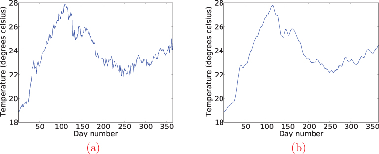
Figure 1.4 Plot of (a) a year’s worth of daily high temperature readings and (b) the temperature readings smoothed over a five-day window.
Reflection 1.8 What general characteristics might make one algorithm for a particular problem better than another algorithm for the same problem?
As was the case in the phone tree problem, the most important hallmark of a good algorithm is speed; given the choice, we almost always want the algorithm that requires the least amount of time to finish. (Would you rather wait five minutes for a web search or half of a second?) But there are other attributes as well that can distinguish one algorithm from another. For example, we saw in Section 1.2 how a long, tedious algorithm can be represented more compactly using a loop; the more compact version is easier to write down and translate into a program. The compact version also requires less space in a computer’s memory. Because the amount of storage space in a computer is limited, we want to create algorithms that use as little of this resource as possible to store both their instructions and their data. Efficient resource usage may also apply to network capacity, as in the phone tree problem on a wireless network. In addition, just as writers and designers strive to create elegant works, computer scientists pride themselves on writing elegant algorithms that are easy to understand and do not contain extraneous steps. And some advanced algorithms are considered to be especially important because they introduce new techniques that can be applied to solve other hard problems.
A smoothing algorithm
To more formally illustrate how we can evaluate the time required by an algorithm, let’s revisit the sequence of temperature readings from the previous section. Often, when we are dealing with large data sets (much longer than this), anomalies can arise due to errors in the sensing equipment, human fallibility, or in the network used to send results to a lab or another collection point. We can mask these erroneous measurements by “smoothing” the data, replacing each value with the mean of the values in a “window” of values containing it. This technique is also useful for extracting general patterns in data by eliminating distracting “bumpy” areas. For example, Figure 1.4 shows a year’s worth of raw temperature data from a floating ocean buoy, next to the same data smoothed over a five day window.

Figure 1.5 Plot of (a) the ten high temperature readings and (b) the temperature readings smoothed over a five-day window.
Let’s design an algorithm for this problem. To get a better sense of the problem and the technique we will use, we will begin by looking at a small example consisting of the first ten temperature readings from the previous section, with an anomalous reading inserted. Specifically, we will replace the 19.1° C reading in the eighth position with an erroneous temperature of 22.1° C:
18.9, 18.9, 19.0, 19.2, 19.3, 19.3, 19.2, 22.1, 19.4, 19.3
The plot of this data in Figure 1.5(a) illustrates this erroneous “bump.”
Now let’s smooth the data by averaging over windows of size five. For each value in the original list, its window will include itself and the four values that come before it. Our algorithm will need to compute the mean of each of these windows, and then add each of these means to a new smoothed list. The last four values do not have four more values after them, so our smoothed list will contain four fewer values than our original list. The first window looks like this:

To find the mean temperature for the window, we sum the five values and divide by 5. The result, 19.06, will represent this window in the smoothed list. The remaining five windows are computed in the same way:

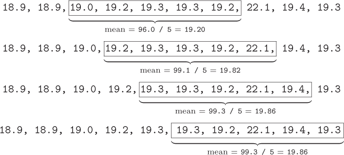
In the end, our list of smoothed temperature readings is:
19.06, 19.14, 19.20, 19.82, 19.86, 19.86
We can see from the plot of this smoothed list in Figure 1.5(b) that the “bump” has indeed been smoothed somewhat.
We can express our smoothing algorithm using notation similar to our previous algorithms. Notice that, to find each of the window means in our smoothing algorithm, we call upon our MEAN algorithm from Section 1.2.
Algorithm SMOOTH
Input: a list of n numbers and a window size w
Create an empty list of mean values.
For each position d, from 1 to n – w + 1, repeat the following:
- invoke the MEAN algorithm on the list of numbers between positions d and d + w – 1;
- append the result to the list of mean values.
Output: the list of mean values
Step 1 creates an empty list to hold the window means. We will append the mean for each window to the end of this list after we compute it. Step 2 uses a loop to compute the means for all of the windows. This loop is similar to the loop in the MEAN algorithm: the variable d takes on the values between 1 and n – w + 1, like t took on each value in the list in the MEAN algorithm. First, d is assigned the value 1, and the mean of the window between positions 1 and 1 + w – 1 = w is added to the list of mean values. Then d is assigned the value 2, and the mean of the window between positions 2 and 2 + w – 1 = w + 1 is added to the list of mean values. And so on, until d takes on the value of n – w + 1, and the mean of the window between positions n – w + 1 and (n – w + 1) + w – 1 = n is added to the list of mean values.
Reflection 1.9 Carry out each step of the SMOOTH algorithm with w = 5 and the ten-element list in our example:
18.9, 18.9, 19.0, 19.2, 19.3, 19.3, 19.2, 22.1, 19.4, 19.3
Compare each step with what we worked out above to convince yourself that the algorithm is correct.
How long does it take?
To determine how much time this algorithm requires to smooth the values in a list, we could implement it as a program and execute it on a computer. However, this approach presents some problems. First, which list(s) do we use for our timing experiments? Second, which value(s) of w do we use? Third, which computer(s) do we use? Will these specific choices give us a complete picture of our algorithm’s efficiency? Will they allow us to predict the time required to smooth other lists on other computers? Will these predictions still be valid ten years from now?
A better way to predict the amount of time required by an algorithm is to count the number of elementary steps that are required. An elementary step is one that always requires the same amount of time, regardless of the input. By counting elementary steps, we can estimate how long an algorithm will take on any computer, relative to another algorithm for the same problem. For example, if algorithm A requires 100 elementary steps while algorithm B requires 300 elementary steps, we know that algorithm A will always be about three times faster than algorithm B, regardless of which computer we run them both on.
Let’s look at which steps in the SMOOTH algorithm qualify as elementary steps. Step 1 qualifies because creating an empty list makes no reference to the input at all. But step 2 does not qualify because its duration depends on the values of n and w, which are both part of the input. Similarly, step 2(a) does not qualify as an elementary step because its duration depends on the time required by the MEAN algorithm, which depends on the value of w. Finding the mean temperature of the window between positions 1 and w will take longer when w is 10 than it will when w is 3. However, each addition and division operation required to compute a mean does qualify as an elementary step because the time required for an arithmetic operation is independent of the operands (up to a point). Step 2(b) also qualifies as an elementary step because, intuitively, adding something to the end of a list should not depend on how many items are in the list (as long as we have direct access to the end of the list).
Reflection 1.10 Based on this analysis, what are the elementary steps in this algorithm? How many times are they each executed?
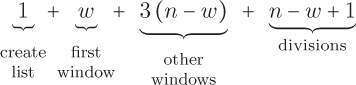
The only elementary steps we have identified are creating a list, appending to a list, and arithmetic operations. Let’s start by counting the number of arithmetic operations that are required. If each window has size five, then we perform five addition operations and one division operation each time we invoke the MEAN algorithm, for a total of six arithmetic operations per window. Therefore, the total number of arithmetic operations is six times the number of windows. In general, the window size is denoted w and there are n – w + 1 windows. So the algorithm performs w additions and one division per window, for a total of (w +1) · (n – w + 1) arithmetic operations. For example, smoothing a list of 365 temperatures with a window size of five days will require (w + 1) · (n – w + 1) = 6 · (365 – 5 + 1) = 2, 166 arithmetic operations. In addition to the arithmetic operations, we create the list once and append to the list once for every window, a total of n – w + 1 times. Therefore, the total number of elementary steps is
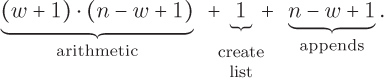
This expression can be simplified a bit to (w + 2) · (n – w + 1) + 1.
This number of elementary steps is called an algorithm’s time complexity. An algorithm’s time complexity is always measured with respect to the size of the input. In this case, the size of the input depends on n, the length of the list, and w, the window size. As we will discuss later, we could simplify this unpleasant time complexity expression by just taking into account the terms that matter when the input gets large. But, for now, we will leave it as is.
Reflection 1.11 Can you think of a way to solve the smoothing problem with fewer arithmetic operations?
A better smoothing algorithm
We can design a more efficient smoothing algorithm, one requiring fewer elementary steps, by exploiting the following simple observation. While finding the sums of neighboring windows in the SMOOTH algorithm, we unnecessarily performed some addition operations more than once. For example, we added the fourth and fifth temperature readings four different times, once in each of the first four windows. We can eliminate this extra work by taking advantage of the relationship between the sums of two contiguous windows. For example, consider the first window:

The sum for the second window must be almost the same as the first window, since they have four numbers in common. The only difference in the second window is that it loses the first 18.9 and gains 19.3. So once we have the sum for the first window (95.3), we can get the sum of the second window with only two additional arithmetic operations: 95.3 – 18.9 + 19.3 = 95.7.

We can apply this process to every subsequent window as well. At the end of the algorithm, once we have the sums for all of the windows, we can simply divide each by its window length to get the final list of means. Written in the same manner as the previous algorithms, our new smoothing algorithm looks like this:
Algorithm SMOOTH 2
Input: a list of n numbers and a window size w
Create an empty list of window sums.
Compute the sum of the first w numbers and append the result to the list of window sums.
For each position d, from 2 to n – w + 1, repeat the following:
- subtract the number in position d – 1 from the previous window sum and then add the number in position d + w – 1;
- append the result to the list of window sums.
For each position d, from 1 to n – w + 1, repeat the following:
- divide the dth window sum by w.
Output: the list of mean values
Step 2 computes the sum for the first window and adds it to a list of window sums. Step 3 then computes the sum for each subsequent window by subtracting the number that is lost from the previous window and adding the number that is gained. Finally, step 4 divides all of the window sums by w to get the list of mean values.
Reflection 1.12 As with the previous algorithm, carry out each step of the SMOOTH 2 algorithm with w = 5 and the ten-element list in our example:
18.9, 18.9, 19.0, 19.2, 19.3, 19.3, 19.2, 22.1, 19.4, 19.3
Does the SMOOTH 2 algorithm actually require fewer elementary steps than our first attempt? Let’s look at each step individually. As before, step 1 counts as one elementary step. Step 2 requires w – 1 addition operations and one append, for a total of w elementary steps. Step 3 performs an addition, a subtraction, and an append for every window but the first, for a total of 3(n – w) elementary steps. Finally, step 4 performs one division operation per window, for a total of n – w + 1 arithmetic operations. This gives us a total of
elementary steps. Combining all of these terms, we find that the time complexity of SMOOTH 2 is 4n – 3w + 2. Therefore, our old algorithm requires
times as many operations as the new one. It is hard to tell from this fraction, but our new algorithm is about w/4 times faster than our old one. To see this, suppose our list contains n = 10,000 temperature readings. The following table shows the value of the fraction for increasing window sizes w.

When w is small, our new algorithm does not make much difference, but the difference becomes quite pronounced when w gets larger. In real applications of smoothing on extremely large data sets containing billions or trillions of items, window sizes can be as high as w = 100, 000. For example, smoothing is commonly used to visualize statistics over DNA sequences that are billions of units long. So our refined algorithm can have a marked impact! Indeed, as we will examine further in Section 6.4, it is often the case that a faster algorithm can reduce the time required for a computation significantly more than faster hardware.
Exercises
1.3.1. The phone tree algorithm depicted in Figure 1.3(c) comes very close to making all of the phone calls in three steps. Is it possible to actually achieve three steps? How?
1.3.2. Suppose the phone tree algorithm illustrated in Figure 1.3(c) was being executed with a large number of people. We saw one call made during the first time step, two calls during the second time step, and three calls during the third time step.
- How many concurrent calls would be made during time steps 4, 5, and 6?
- In general, can you provide a formula (or algorithm) to determine the number of calls made during any time step t?
1.3.3. Describe the most important criterion for evaluating how good an algorithm is. Then add at least one more criterion and describe how it would be applied to algorithms for some everyday problem.
1.3.4. What is the time complexity of the MEAN algorithm on Page 10, in terms of n (the size of the input list)?

1.4 COMPUTERS ARE DUMB
By executing clever algorithms very fast, computers can sometimes appear to exhibit primitive intelligence. In a historic example, in 1997, the IBM Deep Blue computer defeated reigning world champion Garry Kasparov in a six-game match of chess. More recently, in 2011, IBM’s Watson computer beat two champions in the television game show Jeopardy.
The intelligence that we sometimes attribute to computers, however, is actually human intelligence that was originally expressed as an algorithm, and then as a program. Even the statements in a high-level programming language are themselves abstract conveniences built upon a much more rudimentary set of instructions, called a machine language, that a computer can execute natively.
Every statement in a Python program must be translated into a sequence of equivalent machine language instructions before it can be executed by a computer. This process is handled automatically, and somewhat transparently, by either a program called an interpreter or a program called a compiler. An interpreter translates one line of a high-level program into machine language, executes it, then translates the next line and executes it, etc. A compiler instead translates a high-level language program all at once into machine language. Then the compiled machine language program can be executed from start to finish without additional translation. This tends to make compiled programs faster than interpreted ones. However, interpreted languages allow us to more closely interact with a program during its execution. As we will see in Chapter 2, Python is an interpreted programming language.
Inside a computer
The types of instructions that constitute a machine language are based on the internal design of a modern computer. As illustrated in Figure 1.6, a computer essentially consists of one or more processors connected to a memory. A computer’s memory, often called RAM (short for random access memory), is conceptually organized as a long sequence of cells, each of which can contain one unit of information. Each cell is labeled with a unique memory address that allows the processor to reference it specifically. So a computer’s memory is like a huge sequence of equal-sized post office boxes, each of which can hold exactly one letter. Each P.O. box number is analogous to a memory address and a letter is analogous to one unit of information. The information in each cell can represent either one instruction or one unit of data.1 So a computer’s memory stores both programs and the data on which the programs work.
A processor, often called a CPU (short for central processing unit) or a core, contains both the machinery for executing instructions and a small set of memory locations called registers that temporarily hold data values needed by the current instruction. If a computer contains more than one core, as most modern computers do, then it is able to execute more than one instruction at a time. These instructions may be from different programs or from the same program. This means that our definition of an algorithm as a sequence of instructions on Page 7 is not strictly correct. In fact, an algorithm (or a program) may consist of several semi-independent sequences of steps called threads that cooperatively solve a problem.
As illustrated in Figure 1.6, the processors and memory are connected by a communication channel called a bus. When a processor needs a value in memory, it transmits the request over the bus, and then the memory returns the requested value the same way. The bus also connects the processors and memory to several other components that either improve the machine’s efficiency or its convenience, like the Internet and secondary storage devices like hard drives, solid state drives, and flash memory. As you probably know, the contents of a computer’s memory are lost when the computer loses power, so we use secondary storage to preserve data for longer periods of time. We interact with these devices through a “file system” abstraction that makes it appear as if our hard drives are really filing cabinets. When you execute a program or open a file, it is first copied from secondary storage into memory where the processor can access it.
Machine language
The machine language instructions that a processor can execute are very simple. For example, consider something as simple as computing x = 2 + 5. In a program, this statement adds 2 and 5, and stores the result in a memory location referred to by the variable x. But even this is likely to be too complex for one machine language instruction. The machine language equivalent likely, depending on the computer, consists of four instructions. The first instruction loads the value 2 into a register in the processor. The second instruction loads the value 5 into another register in the processor. The third instruction adds the values in these two registers, and stores the result in a third register. Finally, the fourth instruction stores the value in the third register into the memory cell with address x.
Box 1.1: High performance computing
Although today’s computers are extremely fast, there are some problems that are so big that additional power is necessary. These include weather forecasting, molecular modeling and drug design, aerodynamics, and deciphering encrypted data. For these problems, scientists use supercomputers. A supercomputer, or high performance computer, is made of up to tens of thousands of nodes, connected by a very fast data network that shuttles information between nodes. A node, essentially a standalone computer, can contain multiple processors, each with multiple cores. The fastest supercomputers today have millions of cores and a million gigabytes of memory.
To realize the power of these computers, programmers need to supply their cores with a constant stream of data and instructions. The results computed by the individual cores are then aggregated into an overall solution. The algorithm design and programming techniques, known as parallel programming, are beyond the scope of this book, but we provide additional resources at the end of the chapter if you would like to learn more.
From the moment a computer is turned on, its processors are operating in a continuous loop called the fetch and execute cycle (or machine cycle). In each cycle, the processor fetches one machine language instruction from memory and executes it. This cycle repeats until the computer is turned off or loses power. In a nutshell, this is all a computer does. The rate at which a computer performs the fetch and execute cycle is loosely determined by the rate at which an internal clock “ticks” (the processor’s clock rate). The ticks of this clock keep the machine’s operations synchronized. Modern personal computers have clocks that tick a few billion times each second; a 3 gigahertz (GHz) processor ticks 3 billion times per second (“giga” means “billion” and a “hertz” is one tick per second).
So computers, at their most basic level, really are quite dumb; the processor blindly follows the fetch and execute cycle, dutifully executing whatever sequence of simple instructions we give it. The frustrating errors that we yell at computers about are, in fact, human errors. The great thing about computers is not that they are smart, but that they follow our instructions so very quickly; they can accomplish an incredible amount of work in a very short amount of time.
Everything is bits
Our discussion so far has glossed over a very important consideration: in what form does a computer store programs and data? In addition to machine language instructions, we need to store numbers, documents, maps, images, sounds, presentations, spreadsheets, and more. Using a different storage medium for each type of information would be insanely complicated and inefficient. Instead, we need a simple storage format that can accommodate any type of data. The answer is bits. A bit is the simplest possible unit of information, capable of taking on one of only two values: 0 or 1 (or equivalently, off/on, no/yes, or false/true). This simplicity makes both storing information (i.e., memory) and computing with it (e.g., processors) relatively simple and efficient.
Bits are switches
Storing the value of a bit is absurdly simple: a bit is equivalent to an on/off switch, and the value of the bit is equivalent to the state of the switch: off = 0 and on = 1. A computer’s memory is essentially composed of billions of microscopic switches, organized into memory cells. Each memory cell contains 8 switches, so each cell can store 8 bits, called a byte. We represent a byte simply as a sequence of 8 bits, such as 01101001. A computer with 8 gigabytes (GB) of memory contains about 8 billion memory cells, each storing one byte. (Similarly, a kilobyte (KB) is about one thousand bytes, a megabyte (MB) is about one million bytes, and a terabyte (TB) is about one trillion bytes.)
Bits can store anything
A second advantage of storing information with bits is that, as the simplest possible unit of information, it serves as a “lowest common denominator”: all other information can be converted to bits in fairly straightforward manners. Numbers, words, images, music, and machine language instructions are all encoded as sequences of bits before they are stored in memory. Information stored as bits is also said to be in binary notation. For example, consider the following sequence of 16 bits (or two bytes).
0100010001010101
This bit sequence can represent each of the following, depending upon how it is interpreted:
- the integer value 17,493;
- the decimal value 2.166015625;
- the two characters “DU”;
- the Intel machine language instruction
inc x(incis short for “increment”); or - the following 4 × 4 black and white image, called a bitmap (0 represents a white square and 1 represents a black square).

For now, let’s just look more closely at (a). Integers are represented in a computer using the binary number system, which is understood best by analogy to the decimal number system. In decimal, each position in a number has a value that is a power of ten: from right to left, the positional values are 100 = 1, 101 = 10, 102 = 100, etc. The value of a decimal number comes from adding the digits, each first multiplied by the value of its position. So the decimal number 1,831 represents the value
1 × 10³ + 8 × 10² + 3 × 101 + 1 × 100 = 1000 + 800 + 30 + 1.
The binary number system is no different, except that each position represents a power of two, and there are only two digits instead of ten. From right to left, the binary number system positions have values 20 = 1, 21 = 2, 22 = 4, 23 = 8, etc. So, for example, the binary number 110011 represents the value
1 × 25 + 1 × 24 + 0 × 23 + 0 × 22 + 1 × 21 + 1 × 20 = 32 + 16 + 2 + 1 = 51
in decimal. The 16 bit number above, 0100010001010101, is equivalent to
214 + 210 + 26 + 24 + 22 + 20 = 16, 384 + 1, 024 + 64 + 16 + 4 + 1 = 17, 493
in decimal.
Reflection 1.13 To check your understanding, show why the binary number 1001000 is equivalent to the decimal number 72.
This idea can be extended to numbers with a fractional part as well. In decimal, the positions to the right of the decimal point have values that are negative powers of 10: the tenths place has value 10–1 = 0.1, the hundredths place has value 10–2 = 0.01, etc. So the decimal number 18.31 represents the value
1× 101 + 8 × 100 + 3 × 10⁻¹ + 1 × 10–2 = 10 + 8 + 0.3 + 0.01.
Similarly, in binary, the positions to the right of the “binary point” have values that are negative powers of 2. For example, the binary number 11.0011 represents the value
in decimal. This is not, however, how we derived (b) above. Numbers with fractional components are stored in a computer using a different format that allows for a much greater range of numbers to be represented. We will revisit this in Section 2.2.
Reflection 1.14 To check your understanding, show why the binary number 1001.101 is equivalent to the decimal number 9 5/8.
Binary computation is simple
A third advantage of binary is that computation on binary values is exceedingly easy. In fact, there are only three fundamental operators, called and, or, and not. These are known as the Boolean operators, after 19th century mathematician George Boole, who is credited with inventing modern mathematical logic, now called Boolean logic or Boolean algebra.
To illustrate the Boolean operators, let the variables a and b each represent a bit with a value of 0 or 1. Then a and b is equal to 1 only if both a and b are equal to 1; otherwise a and b is equal to 0.2 This is conveniently represented by the following truth table:
a |
b |
a and b |
0 |
0 |
0 |
0 |
1 |
0 |
1 |
0 |
0 |
1 |
1 |
1 |
Each row of the truth table represents a different combination of the values of a and b. These combinations are shown in the first two columns. The last column of the truth table contains the corresponding values of a and b. We see that a and b is 0 in all cases, except where both a and b are 1. If we let 1 represent “true” and 0 represent “false,” this conveniently matches our own intuitive meaning of “and.” The statement “the barn is red and white” is true only if the barn both has red on it and has white on it.
Second, a or b is equal to 1 if at least one of a or b is equal to 1; otherwise a or b is equal to 0. This is represented by the following truth table:
a |
b |
a or b |
0 |
0 |
0 |
0 |
1 |
1 |
1 |
0 |
1 |
1 |
1 |
1 |
Notice that a or b is 1 even if both a and b are 1. This is different from our normal understanding of “or.” If we say that “the barn is red or white,” we usually mean it is either red or white, not both. But the Boolean operator can mean both are true. (There is another Boolean operator called “exclusive or” that does mean “either/or,” but we won’t get into that here.)
Finally, the not operator simply inverts a bit, changing a 0 to 1, or a 1 to 0. So, not a is equal to 1 if a is equal to 0, or 0 if a is equal to 1. The truth table for the not operator is simple:
a |
not a |
0 |
1 |
1 |
0 |
With these basic operators, we can build more complicated expressions. For example, suppose we wanted to find the value of the expression not a and b. (Note that the not operator applies only to the variable immediately after it, in this case a, not the entire expression a and b. For not to apply to the expression, we would need parentheses: not (a and b).) We can evaluate not a and b by building a truth table for it. We start by listing all of the combinations of values for a and b, and then creating a column for not a, since we need that value in the final expression:
a |
b |
not a |
0 |
0 |
1 |
0 |
1 |
1 |
1 |
0 |
0 |
1 |
1 |
0 |
Then, we create a column for not a and b by anding the third column with the second.
a |
b |
not a |
not a and b |
0 |
0 |
1 |
0 |
0 |
1 |
1 |
1 |
1 |
0 |
0 |
0 |
1 |
1 |
0 |
0 |
So we find that not a and b is 1 only when a is 0 and b is 1. Or, equivalently, not a and b is true only when a is false and b is true. (Think about that for a moment; it makes sense, doesn’t it?)
The universal machine
The previous advantages of computing in binary—simple switch implementations, simple Boolean operators, and the ability to encode anything—would be useless if we could not actually compute in binary everything we want to compute. In other words, we need binary computation (i.e., Boolean algebra) to be universal: we need to be able to compute any computable problem by using only the three basic Boolean operators. But is such a thing really possible? And what do we mean by any computable problem? Can we really perform any computation at all—a web browser, a chess-playing program, Mars rover software—just by converting it to binary and using the three elementary Boolean operators to get the answer?
Fortunately, the answer is yes, when we combine logic circuits with a sufficiently large memory and a simple controller called a finite state machine (FSM) to conduct traffic. A finite state machine consists of a finite set of states, along with transitions between states. A state represents the current value of some object or the degree of progress made toward some goal. For example, a simple elevator, with states representing floors, is a finite state machine, as illustrated below.


States are represented by circles and transitions are arrows between circles. In this elevator, there are only up and down buttons (no ability to choose your destination floor when you enter). The label on each transition represents the button press event that causes the transition to occur. For example, when we are on the ground floor and the down button is pressed, we stay on the ground floor. But when the up button is pressed, we transition to the first floor. Many other simple systems can also be represented by finite state machines, such as vending machines, subway doors, traffic lights, and tool booths. The implementation of a finite state machine in a computer coordinates the fetch and execute cycle, as well as various intermediate steps involved in executing machine language instructions.
This question of whether a computational system is universal has its roots in the very origins of computer science itself. In 1936, Alan Turing proposed an abstract computational model, now called a Turing machine, that he proved could compute any problem considered to be mathematically computable. As illustrated in Figure 1.7, a Turing machine consists of a control unit containing a finite state machine that can read from and write to an infinitely long tape. The tape contains a sequence of “cells,” each of which can contain a single character. The tape is initially inscribed with some sequence of input characters, and a pointer attached to the control unit is positioned at the beginning of the input. In each step, the Turing machine reads the character in the current cell. Then, based on what it reads and the current state, the finite state machine decides whether to write a character in the cell and whether to move its pointer one cell to the left or right. Not unlike the fetch and execute cycle in a modern computer, the Turing machine repeats this simple process as long as needed, until a designated final state is reached. The output is the final sequence of characters on the tape.
The Turing machine still stands as our modern definition of computability. The Church-Turing thesis states that a problem is computable if and only if it can be computed by a Turing machine. Any mechanism that can be shown to be equivalent in computational power to a Turing machine is considered to be computationally universal, or Turing complete. A modern computer, based on Boolean logic and a finite state machine, falls into this category.
Exercises
1.4.1. Show how to convert the binary number 1101 to decimal.
1.4.2. Show how to convert the binary number 1111101000 to decimal.
1.4.3. Show how to convert the binary number 11.0011 to decimal.
1.4.4. Show how to convert the binary number 11.110001 to decimal.
1.4.5. Show how to convert the decimal number 22 to binary.
1.4.6. Show how to convert the decimal number 222 to binary.
1.4.7. See how closely you can represent the decimal number 0.1 in binary using six places to the right of the binary point. What is the actual value of your approximation?
1.4.8. Consider the following 6 × 6 black and white image. Describe two plausible ways to represent this image as a sequence of bits.

1.4.9. Design a truth table for the Boolean expression not (a and b).
1.4.10. Design a truth table for the Boolean expression not a or not b. Compare the result to the truth table for not (a and b). What do you notice? The relationship between these two Boolean expressions is one of De Morgan’s laws.
1.4.11. Design a truth table for the Boolean expression not a and not b. Compare the result to the truth table for not (a or b). What do you notice? The relationship between these two Boolean expressions is the other of De Morgan’s laws.
1.4.12. Design a finite state machine that represents a highway toll booth controlling a single gate.
1.4.13. Design a finite state machine that represents a vending machine. Assume that the machine only takes quarters and vends only one kind of drink, for 75 cents. First, think about what the states should be. Then design the transitions between states.

Figure 1.8 An expanded (from Figure 1.2) illustration of the layers of functional abstraction in a computer.
1.5 SUMMARY
In the first chapter, we developed a top-to-bottom view of computation at many layers of abstraction. As illustrated in Figure 1.8, we start with a well-defined problem and solve it by designing an algorithm. This step is usually the most difficult by far. Professional algorithm designers rely on experience, creativity, and their knowledge of a battery of general design techniques to craft efficient, correct algorithms. In this book, we will only scratch the surface of this challenging field. Next, an algorithm can be programmed in a high-level programming language like Python, which is translated into machine language before it can be executed on a computer. The instructions in this machine language program may either be executed directly on a processor or request that the operating system do something on their behalf (e.g., saving a file or allocating more memory). Each instruction in the resulting computation is implemented using Boolean logic, controlled by a finite state machine.
Try to keep this big picture in mind as you work through this book, especially the role of abstraction in effective problem solving. The problems we will tackle are modest, but they should give you an appreciation for the big questions and techniques used by computer scientists, and some of the fascinating interdisciplinary opportunities that await you.
1.6 FURTHER DISCOVERY
The epigraph at the beginning of this chapter is from an article by computer scientists Michael Fellows and Ian Parberry [13]. A similar quote is often attributed to the late Dutch computer scientist Edsger Dijkstra.
There are several excellent books available that give overviews of computer science and how computers work. In particular, we recommend The Pattern on the Stone by Danny Hillis [18], Algorithmics by David Harel [17], Digitized by Peter Bentley [5], and CODE: The Hidden Language of Computer Hardware and Software by Charles Petzold [40].
There really are drifting buoys in the world’s oceans that are constantly taking temperature readings to monitor climate change. For example, see
http://www.coriolis.eu.org.
A list of the fastest supercomputers in the world is maintained at
http://top500.org.
You can learn more about IBM’s Deep Blue supercomputer at
http://www-03.ibm.com/ibm/history/ibm100/us/en/icons/deepblue/
and IBM’s Watson supercomputer at
http://www.ibm.com/smarterplanet/us/en/ibmwatson/.
To learn more about high performance computing in general, we recommend looking at the website of the National Center for Supercomputing Applications (NCSA) at the University of Illinois, one of the first supercomputer centers funded by the National Science Foundation, at
http://www.ncsa.illinois.edu/about/faq.
There are several good books available on the life of Alan Turing, the father of computer science. The definitive biography, Alan Turing: The Enigma, was written by Andrew Hodges [20].
1In reality, each instruction or unit of data usually occupies multiple contiguous cells.
2In formal Boolean algebra, a and b is usually represented a ∧ b, a or b is usually represented a ∨ b, and not a is usually represented as ¬a.