
CHAPTER 6
Text, documents, and DNA
So, here’s what I can say: the Library of Congress has more than 3 petabytes of digital collections. What else I can say with all certainty is that by the time you read this, all the numbers — counts and amount of storage — will have changed.
Leslie Johnston, former Chief of Repository Development, Library of Congress
Blog post (2012)
The roughly 2000 sequencing instruments in labs and hospitals around the world can collectively sequence 15 quadrillion nucleotides per year, which equals about 15 petabytes of compressed genetic data. A petabyte is 250 bytes, or in round numbers, 1000 terabytes. To put this into perspective, if you were to write this data onto standard DVDs, the resulting stack would be more than 2 miles tall. And with sequencing capacity increasing at a rate of around three- to fivefold per year, next year the stack would be around 6 to 10 miles tall. At this rate, within the next five years the stack of DVDs could reach higher than the orbit of the International Space Station.
Michael C. Schatz and Ben Langmead
The DNA Data Deluge (2013)
NEW technologies are producing data at an incredible rate, sometimes faster than it can be stored and analyzed. By some accounts, Google plans to have scanned every book in existence by the end of this decade. Sequencing of the approximately three billion base pairs of the human genome took 10 years when first published in 2000, but can now be done in less than a week. Social scientists currently have at their disposal a steady stream of data from online social networks. Analyses of data of these magnitudes, most of which is stored as text, requires computational tools. In this chapter, we will discuss the fundamental algorithmic techniques for developing these tools. We will look at how text is represented in a computer, how to read text from both files and the web, and develop algorithms to process and analyze textual data.
6.1 COUNTING WORDS
As we have already seen, we can store text as a sequence of characters called a string. A string constant (also called a string literal), such as 'You got it!', is enclosed in either single quotes (') or double quotes ("). We have also seen that string values can be assigned to variable names, passed as parameters, and compared to each other just like numbers, as illustrated in the following silly functions.
def roar(n):
    return 'r' + ('o' * n) + ('a' * n) + 'r!'

def speak(animal):
    if animal == 'cat':
        word = 'meow.'
    elif animal == 'dog':
        word = 'woof.'
    else:
        word = roar(10)

     print('The', animal, 'says', word)

speak('monkey')
Reflection 6.1 What is printed by the code above? Make sure you understand why.
Like a Turtle, a string is an object, an instance of a class named str. As such, a string is also another example of an abstract data type. Recall that an abstract data type hides the implementation details of how its data is stored, allowing a programmer to interact with it through a set of functions called methods. As we will discuss in Section 6.3, strings are actually stored as binary sequences, yet we can interact with them in a very natural way.
There are several methods available for strings.1 For example, the upper() method returns a new string with all the lower case characters in the old string capitalized. For example,
>>> pirate = 'Longbeard'
>>> newName = pirate.upper()
>>> newName
'LONGBEARD'
Remember that, when using methods, the name of the object, in this case the string object named pirate, precedes the name of the method.
Smaller strings contained within larger strings are called substrings. We can use the operators in and not in to test whether a string contains a particular substring. For example, the conditions in each of the following if statements are true.
>>> if 'bear' in pirate:
...     print('There is a bear in Longbeard.')
...
There is a bear in Longbeard.
>>> if 'beer' not in pirate:
...     print('There is no beer in Longbeard.')
...
There is no beer in Longbeard.
Two particularly useful methods that deal with substrings are replace and count. The replace method returns a new string with all occurrences of one substring replaced with another substring. For example,
>>> newName = pirate.replace('Long', 'Short')
>>> newName
'Shortbeard'
>>> quote = 'Yo-ho-ho, and a bottle of rum!'
>>> quote2 = quote.replace(' ', '')
>>> quote2
'Yo-ho-ho,andabottleofrum!'
The second example uses the replace method to delete spaces from a string. The second parameter to replace, quotes with nothing in between, is called the empty string, and is a perfectly legal string containing zero characters.
Reflection 6.2 Write a statement to replace all occurrences of brb in a text with be right back.
>>> txt = 'Hold on brb'
>>> txt.replace('brb', 'be right back')
'Hold on be right back'
The count method returns the number of occurrences of a substring in a string. For example,
>>> pirate.count('ear')
1
>>> pirate.count('eye')
0
We can count the number of words in a text by counting the number of “whitespace” characters, since almost every word must be followed by a space of some kind. Whitespace characters are spaces, tabs, and newline characters, which are the hidden characters that mark the end of a line of text. Tab and newline characters are examples of non-printable control characters. A tab character is denoted by the two characters and a newline character is denoted by the two characters
. The wordCount1 function below uses the count method to return the number of whitespace characters in a string named text.
def wordCount1(text):
    """Approximate the number of words in a string by counting
       the number of spaces, tabs, and newlines.

    Parameter:
        text: a string object

    Return value: the number of spaces, tabs and newlines in text
    """

    return text.count(' ') + text.count('	') + text.count('
')

def main():
    shortText = 'This⌴is⌴not⌴long. ⌴⌴But⌴it⌴will⌴do. ⌴
' +
                'All⌴we⌴need⌴is⌴a⌴few⌴sentences.'
    wc = wordCount1(shortText)
    print(wc)

main()
In the string shortText above, we explicitly show the space characters (⌴) and break it into two parts because it does not fit on one line.
Reflection 6.3 In a Python shell, try entering
print('Two tabs		here.    Two newlines

here.')
to see the effects of the and
characters.
Reflection 6.4 What answer does the wordCount1 function give in the example above? Is this the correct answer? If not, why not?
The wordCount1 function returns 16, but there are actually only 15 words in shortText. We did not get the correct answer because there are two spaces after the first period, a space and newline character after the second period, and nothing after the last period. How can we fix this? If we knew that the text contained no newline characters, and was perfectly formatted with one space between words, two spaces between sentences, and no space at the end, then we could correct the above computation by subtracting the number of instances of two spaces in the text and adding one for the last word:
def wordCount2(text):
    """ (docstring omitted) """

    return text.count(' ') - text.count('     ') + 1
But most text is not perfectly formatted, so we need a more sophisticated approach.
Reflection 6.5 If you were faced with a long text, and could only examine one character at a time, what algorithm would you use to count the number of words?
As a starting point, let’s think about how the count method must work. To count the number of instances of some character in a string, the count method must examine each character in the string, and increment an accumulator variable for each one that matches.
To replicate this behavior, we can iterate over a string with a for loop, just as we have iterated over ranges of integers. For example, the following for loop iterates over the characters in the string shortText. Insert this loop into the main function above to see what it does.
for character in shortText:
    print(character)
In this loop, each character in the string is assigned to the index variable character in order. To illustrate this, we have the body of the loop simply print the character assigned to the index variable. Given the value assigned to shortText in the main function above, this loop will print
T
h
i
⋮     (middle omitted)
e
s
.
To count whitespace characters, we can use the same loop but, in the body of the loop, we need to increment a counter each time the value of character is equal to a whitespace character:
def wordCount3(text):
    """ (docstring omitted) """

    count = 0
    for character in text:
        if character == ' ' or character == '	' or character == '
':
            count = count + 1
    return count
Reflection 6.6 What happens if we replace the or operators with and operators?
Alternatively, this if condition can be simplified with the in operator:
if character in '
':
Reflection 6.7 What answer does the wordCount3 function give when it is called with the parameter shortText that we defined above?
When we call this function with shortText, we get the same answer that we did with wordCount1 (16) because we have simply replicated that function’s behavior.
Reflection 6.8 Now that we have a baseline word count function, how can we make it more accurate on text with extra spaces?
To improve upon wordCount3, we need to count only the first whitespace or newline character in any sequence of such characters.
Reflection 6.9 If the value of character is a space, tab, or newline, how can we tell if it is the first in a sequence of such characters? (Hint: if it is the first, what must the previous character not be?)
If the value of character is a whitespace or newline character, we know it is the first in a sequence if the previous character was not one of these characters. So we need to also keep track of the previous character and check its value in the if statement. If we use a variable named prevCharacter to store this value, we would need to change the if statement to
if character in '
' and prevCharacter not in '
':
    count = count + 1
Reflection 6.10 Where should we assign prevCharacter a value?
We need to assign the current value of character to prevCharacter at the end of each iteration because this current value of character will be the previous character during the next iteration. With these pieces added, our revised wordCount4 looks like this:
def wordCount4(text):
    """ (docstring omitted) """

    count = 0
    prevCharacter = ' '
    for character in text:
        if character in '
' and prevCharacter not in '
':
            count = count + 1
        prevCharacter = character
    return count
The one remaining piece, included above, is to initialize prevCharacter to something before the loop so that the if condition makes sense in the first iteration.
Reflection 6.11 What happens if we do not initialize prevCharacter before the loop? Why did we initialize prevCharacter to a space? Does its initial value matter?
Let’s consider two possibilities for the first character in text: either it is a whitespace character, or it is not. If the first character in text is not a whitespace or newline character (as would normally be the case), then the first part of the if condition (character in '
') will be false. Therefore, the initial value of prevCharacter does not matter. On the other hand, if the first value assigned to character is a whitespace or newline character, then the first part of the if condition will be true. But we want to make sure that this character does not count as ending a word. Setting prevCharacter to a space initially will ensure that the second part of the if condition (prevCharacter not in '
') is initially false, and prevent count from being incremented.
Reflection 6.12 Are there any other values that would work for the initial value of prevCharacter?
Finally, we need to deal with the situation in which the text does not end with a whitespace character. In this case, the final word would not have been counted, so we need to increment count by one.
Reflection 6.13 How can we tell if the last character in text is a whitespace or newline character?
Since prevCharacter will be assigned the last character in text after the loop completes, we can check its value after the loop. If it is a whitespace character, then the last word has already been counted; otherwise, we need to increment count. So the final function looks like this:
def wordCount5(text):
    """Count the number of words in a string.

    Parameter:
        text: a string object

    Return value: the number of words in text
    """

    count = 0
    prevCharacter = ' '
    for character in text:
        if character in '
' and prevCharacter not in '
':
            count = count + 1
        prevCharacter = character
    if prevCharacter not in '
':
        count = count + 1
    return count
Although our examples have used short strings, our function will work on any size string we want. In the next section, we will see how to read an entire text file or web page into a string, and then use our word count function, unchanged, to count the words in the file. In later sections, we will design similar algorithms to carry out more sophisticated analyses of text files containing entire books and long sequences of DNA.
Exercises
6.1.1. Write a function
twice(text)
that returns the string text repeated twice, with a space in between. For example, twice('bah') should return the string 'bah bah'.
6.1.2. Write a function
repeat(text, n)
that returns a string that is n copies of the string text. For example, repeat('AB', 3) should return the string 'ABABAB'.
vowels(word)
that uses the count method to return the number of vowels in the string word. (Note that word may contain upper and lower case letters.)
nospaces(sentence)
that uses the replace string method to return a version of the string sentence in which all the spaces have been replaced by the underscore (_) character.
6.1.5. Write a function
txtHelp(txt)
that returns an expanded version of the string txt, which may contain texting abbreviations like “brb” and “lol.” Your function should expand at least four different texting abbreviations. For example, txtHelp('imo u r lol brb') might return the string 'in my opinion you are laugh out loud be right back'.
6.1.6. Write a function
letters(text)
that prints the characters of the string text, one per line. For example letters('abc') should print
a
b
c
6.1.7. Write a function
count(text, letter)
that returns the number of occurrences of the one-character string named letter in the string text, without using the count method. (Use a for loop instead.)
6.1.8. Write a function
vowels(word)
that returns the same result as Exercise 6.1.3 without using the count method. (Use a for loop instead.)
6.1.9. Write a function
sentences(text)
that returns the number of sentences in the string text. A sentence may end with a period, question mark, or exclamation point. It may also end with multiple punctuation marks, such as '!!!' or '?!'.
6.1.10. Write a function
nospaces(sentence)
that returns the same result as Exercise 6.1.4 without using the replace method. (Hint: use a for loop and the string concatenation operator (+) inside the loop to build up a new string. We will see more examples like this in Section 6.3.)
6.1.11. When bits are sent across a network, they are sometimes corrupted by interference or errors. Adding some redundant bits to the end of the transmission can help to detect these errors. The simplest error detection algorithm is known as parity checking. A bit string has even parity if it has an even number of ones, and odd parity otherwise. In an even parity scheme, the sender adds a single bit to the end of the bit string so that the final bit string has an even number of ones. For example, if we wished to send the data 1101011, would actually send 11010111 instead so that the bit string has an even number of ones. If we wished to send 1101001 instead, we would actually send 11010010. The receiver then checks whether the received bit string has even parity; if it does not, then an error must have occurred so it requests a retransmission.
(a) Parity can only detect very simple errors. Give an example of an error that cannot be detected by an even parity scheme.
(b) Propose a solution that would detect the example error you gave above.
(c) In the next two problems, we will pretend that bits are sent as strings (they are not; this would be terribly inefficient). Write a function
evenParity(bits)
that uses the count method to return True if the string bits has even parity and False otherwise. For example, evenParity('110101') should return True and evenParity('110001') should return False.
(d) Now write the evenParity function without using the count method.
(e) Write a function
makeEvenParity(bits)
that returns a string consisting of bits with one additional bit concatenated so that the returned string has even parity. Your function should call your evenParity function. For example, makeEvenParity('110101') should return '1101010' and makeEvenParity('110001') should return '1100011'.
6.2 TEXT DOCUMENTS
In real applications, we read text from files stored on a hard drive or a flash drive. Like everything else in a computer system, files are sequences of bits. But we interact with files as abstractions, electronic documents containing information such as text, spreadsheets, or images. These abstractions are mediated by a part of the operating system called a file system. The file system organizes files in folders in a hierarchical fashion, such as in the simplified view of a Mac OS X file system in Figure 6.1. Hierarchical structures like this are called trees. The top of the tree is called the root and branches are called children. Elements of the tree with no children are called leaves. In a file system, a folder can have children, consisting of files or other folders residing inside it, whereas files are always leaves.
Below the root in this figure is a folder named Users where every user of the computer has a home folder labeled with his or her name, say george. In the picture above, this home folder contains two subfolders named CS 111 and HIST 216. We can represent the location of a file with the path one must follow to get there from the root. For example, the path to the file dna.py is /Users/george/CS 111/dna.py. The initial slash character represents the root, whereas the others simply divide layers. Any path without the first slash character is considered to be a relative path, relative to the current working directory set by the operating system. For example, if the current working directory were /Users/george, then dna.py could be specified with the relative path CS 111/dna.py.
Reading from text files
In Python, a file is represented by an abstraction called a file object. We associate a file with a file object by using the open function, which takes a file name or a path as an argument and returns a file object. For example, the following statement associates the file object named inputFile with the file named mobydick.txt in the current working directory.2
inputFile = open('mobydick.txt', 'r')
The second argument to open is the mode to use when working with the file; 'r' means that we want to read from the file. By default, every file is assumed to contain text.

Figure 6.1 A Finder window in Mac OS X and the partial corresponding tree representation. Ovals represent folders and rectangles represent files.
The read method of a file object reads the entire contents of a file into a string. For example, the following statement would read the entire text from the file into a string assigned to the variable named text.
text = inputFile.read()
When we are finished with a file, it is important that we close it. Closing a file signals to the operating system that we are done using it, and ensures that any memory allocated to the file by the program is released. To close a file, we simply use the file object’s close method:
inputFile.close()
Let’s look at an example that puts all of this together. The following function reads in a file with the given file name and returns the number of words in the file using our wordCount5 function.
def wcFile(fileName):
    """Return the number of words in the file with the given name.

    Parameter:
        fileName: the name of a text file

    Return value: the number of words in the file
    """

    textFile = open(fileName, 'r', encoding = 'utf-8')
    text = textFile.read()
    textFile.close()

    return wordCount5(text)
The optional encoding parameter to the open function indicates how the bits in the file should be interpreted (we will discuss what UTF-8 is in Section 6.3).
Reflection 6.14 How many words are there in the file mobydick.txt?
Now suppose we want to print a text file, formatted with line numbers to the left of each line. A “line” is defined to be a sequence of characters that end with a newline ('
') character. Since we need to print a line number to the left of every line, this problem would be much more easily solved if we could read in a file one line at a time. Fortunately, we can. In the same way that we can iterate over a range of integers or the characters of a string, we can iterate over the lines in a file. When we use a file object as the sequence in a for loop, the index variable is assigned a string containing each line in the file, one line per iteration. For example, the following code prints each line in the file object named textFile:
for line in textFile:
    print(line)
In each iteration of this loop, the index variable named line is assigned the next line in the file, which is then printed in the body of the loop. We can easily extend this idea to our line-printing problem:
def lineNumbers(fileName):
    """Print the contents of the file with the given name
       with each line preceded by a line number.

     Parameter:
         fileName: the name of a text file

     Return value: None
     """

     textFile = open(fileName, 'r', encoding = 'utf-8')
     lineCount = 1
     for line in textFile:
         print('{0:<5} {1}'.format(lineCount, line[:-1]))
         lineCount = lineCount + 1
     textFile.close()
The lineNumbers function combines an accumulator with a for loop that reads the text file line by line. After the file is opened, the accumulator variable lineCount is initialized to one. Inside the loop, each line is printed using a format string that precedes the line with the current value of lineCount. At the end of the loop, the accumulator is incremented and the loop repeats.
Reflection 6.15 Why does the function print line[:-1] instead of line in each iteration? What happens if you replace line[:-1] with line?
Reflection 6.16 How would the output change if lineCount was instead incremented in the loop before calling print?
Reflection 6.17 How many lines are there in the file mobydick.txt?
Writing to text files
We can also create new files or write to existing ones. For example, instead of printing a file formatted with line numbers, we might want to create a new version of the file that includes line numbers. To write text to a new file, we first have to open it using 'w' (“write”) mode:
newTextFile = open('newfile.txt', 'w')
Opening a file in this way will create a new file named newfile.txt, if a file by that name does not exist, or overwrite the file by that name if it does exist. (So be careful!) To append to the end of an existing file, use the 'a' (“append”) mode instead. Once the file is open, we can write text to it using the write method:
newTextFile.write('Hello.
')
The write method does not write a newline character at the end of the string by default, so we have to include one explicitly, if one is desired.
The following function illustrates how we can modify the lineNumbers function so that it writes the file with line numbers directly to another file instead of printing it.
def lineNumbersFile(fileName, newFileName):
    """Write the contents of the file fileName to the file
       newFileName, with each line preceded by a line number.

    Parameters:
        fileName: the name of a text file
        newFileName: the name of the output text file

    Return value: None
    """

    textFile = open(fileName, 'r', encoding = 'utf-8')
    newTextFile = open(newFileName, 'w')
    lineCount = 1
    for line in textFile:
        newTextFile.write('{0:<5} {1}
'.format(lineCount, line[:-1]))
        lineCount = lineCount + 1
    textFile.close()
    newTextFile.close()
Remember to always close the new file when you are done. Closing a file to which we have written ensures that the changes have actually been written to the drive. To improve efficiency, an operating system does not necessarily write text out to the drive immediately. Instead, it usually waits until a sufficient amount builds up, and then writes it all at once. Therefore, if you forget to close a file and your computer crashes, your program’s last writes may not have actually been written. (This is one reason why we sometimes have trouble with corrupted files after a computer crash.)
Reading from the web
The ability to read files allows us to conveniently apply the functions that we have already developed to real data that we download from the web. It would be even more convenient, however, if we could read some data directly from the web rather than having to manually download it and then read it with our program. Conveniently, we can do that in Python too.
The urllib.request module contains a function named urlopen that returns a file object abstraction for a web page that is similar to the one returned by the open function. The urlopen function takes as a parameter the address of the web page we wish to access. A web page address is formally known as a URL, short for Uniform Resource Locator, and normally begins with the prefix http:// (“http” is short for “hypertext transfer protocol”). For example, to open the main web page at python.org, we can do the following:
>>> import urllib.request as web
>>> webpage = web.urlopen('http://python.org')
Once we have the file object, we can read from it just as we did earlier.
>>> text = webpage.read()
>>> webpage.close()
Behind the scenes, the Python interpreter communicates with a web server over the Internet to read this web page. But thanks to the magic of abstraction, we did not have to worry about any of those details.
Because the urlopen function does not accept an encoding parameter, the read function cannot tell how the text of the web page is encoded. Therefore, read returns a bytes object instead of a string. A bytes object contains a sequence of raw bytes that are not interpreted in any particular way. To convert the bytes object to a string before we print it, we can use the decode method, as follows:
>>> print(text.decode('utf-8'))
<!doctype html>
  .
  .
  .
(Again, we will see what UTF-8 is in Section 6.3.) What you see when you print text is HTML (short for hypertext markup language) code for the python.org home page. HTML is the language in which most web pages are written.
We can download data files from the web in the same way if we know the correct URL. For example, the U.S. Food and Drug Administration (FDA) lists recalls of products that it regulates at http://www.fda.gov/Safety/Recalls/default.htm. The raw data behind this list is also available, so we can write a program that reads and parses it to gather statistics about recalls over time. Let’s first take a look at what the data looks like. Because the file is quite long, we will initially print only the first twenty lines by calling the readline method, which just reads a single line into a string, in a for loop:
>>> url = 'http://www.fda.gov/DataSets/Recalls/RecallsDataSet.xml'
>>> webpage = web.urlopen(url)
>>> for i in range(20):
...     line = webpage.readline()
...     print(line.decode('utf-8'))
...
This loop prints something like the following.
<?xml version="1.0" encoding="UTF-8" ?>

<RECALLS_DATA>
<PRODUCT>
   <DATE>Mon, 11 Aug 2014 00:00:00 -0400</DATE>
   <BRAND_NAME><![CDATA[Good Food]]></BRAND_NAME>
   <PRODUCT_DESCRIPTION><![CDATA[Carob powder]]></PRODUCT_DESCRIPTION>
   <REASON><![CDATA[Salmonella]]></REASON>
   <COMPANY><![CDATA[Goodfood Inc.]]></COMPANY>
   <COMPANY_RELEASE_LINK>http://www.fda.gov/Safety/Recalls/ucm40969.htm
       </COMPANY_RELEASE_LINK>
   <PHOTOS_LINK></PHOTOS_LINK>
</PRODUCT>
  .
  .
  .
</RECALLS_DATA>
This file is in a common format called XML (short for extensible markup language). In XML, data elements are enclosed in matching pairs of tags. In this file, each product recall is enclosed in a pair of <PRODUCT> … </PRODUCT> tags. Within that element are other elements enclosed in matching tags that give detailed information about the product.
Reflection 6.18 Look at the (fictitious) example product above enclosed in the <PRODUCT> … </PRODUCT> tags. What company made the product? What is the product called? Why was it recalled? When was it recalled?
Before we can do anything useful with the data in this file, we need to be able to identify individual product recall descriptions. Notice that the file begins with a header line that describes the version of XML and the text encoding. Following some blank lines, we next notice that all of the recalls are enclosed in a matching pair of <RECALLS_DATA> … </RECALLS_DATA> tags. So to get to the first product, we need to read until we find the <RECALLS_DATA> tag. We can do this with a while loop:
url = 'http://www.fda.gov/DataSets/Recalls/RecallsDataSet.xml'
webpage = web.urlopen(url)

line = ''
while line[:14] != '<RECALLS_DATA>':
    line = webpage.readline()
    line = line.decode('utf-8')
Implicit in the file object abstraction is a file pointer that keeps track of the position of the next character to be read. So this while loop helpfully moves the file pointer to the beginning of the line after the <RECALLS_DATA> tag.
Reflection 6.19 Why do we have to initialize line before the loop?
Reflection 6.20 Why will line != '<RECALLS_DATA>' not work as the condition in the while loop? (What control character is “hiding” at the end of that line?)
To illustrate how we can identify a product element, let’s write an algorithm to print just the first one. We can then put this code into a loop to print all of the product elements, or modify the code to do something more interesting with the data. Assuming that the file pointer is now pointing to the beginning of a <PRODUCT> tag, we want to print lines until we find the matching </PRODUCT> tag. This can be accomplished with another while loop:
line = webpage.readline()             # read the <PRODUCT> line
line = line.decode('utf-8')
while line[:10] != '</PRODUCT>':      # while we don't see </PRODUCT>
    print(line.rstrip())              # print the line
    line = webpage.readline()         # read the next line
    line = line.decode('utf-8')
print(line.rstrip())                  # print the </PRODUCT> line
The two statements before the while loop read and decode one line of XML data, so that the condition in the while loop makes sense when it is first tested. The while loop then iterates while we have not read the </PRODUCT> tag that marks the end of the product element. Inside the loop, we print the line and then read the next line of data. Since the loop body is not executed when line[:10] == '</PRODUCT>', we add another call to the print function after the loop to print the closing tag.
Reflection 6.21 Why do we call line.rstrip() before printing each line? (What happens if we omit the call to rstrip?)
Reflection 6.22 What would happen if we did not call readline inside the loop?
Finally, let’s put this loop inside another loop to print and count all of the product elements. We saw earlier that the product elements are enclosed within <RECALLS_DATA> … </RECALLS_DATA> tags. Therefore, we want to print product elements while we do not see the closing </RECALLS_DATA> tag.
def printProducts():
    """Print the products on the FDA recall list.

     Parameters: none

     Return value: None
     """

     url = 'http://www.fda.gov/DataSets/Recalls/RecallsDataSet.xml'
     webpage = web.urlopen(url)

     line = ''

     while line[:14] != '<RECALLS_DATA>':   # read past headers
         line = webpage.readline()
         line = line.decode('utf-8')

     productNum = 1
     line = webpage.readline()              # read first <PRODUCT> line
     line = line.decode('utf-8')
     while line[:15] != '</RECALLS_DATA>':  # while more products
         print(productNum)
         while line[:10] != '</PRODUCT>':   # print one product element
             print(line.rstrip())
             line = webpage.readline()
             line = line.decode('utf-8')
         print(line.rstrip())
         productNum = productNum + 1
         line = webpage.readline()          # read next <PRODUCT> line
         line = line.decode('utf-8')

     webpage.close()
The new while loop and the new statements that manage the accumulator to count the products are marked in red. A loop within a loop, often called a nested loop, can look complicated, but it helps to think of the previously written inner while loop (the five black statements in the middle) as a functional abstraction that prints one product. The outer loop repeats this segment while we do not see the final </RECALLS_DATA> tag. The condition of the outer loop is initialized by reading the first <PRODUCT> line before the loop, and the loop moves toward the condition becoming false by reading the next <PRODUCT> (or </RECALLS_DATA>) line at the end of the loop.
Although our function only prints the product information, it provides a framework in which to do more interesting things with the data. Exercise 6.5.7 in Section 6.5 asks you to use this framework to compile the number of products recalled for a particular reason in a particular year.
Exercises
6.2.1. Modify the lineNumbers function so that it only prints a line number on every tenth line (for lines 1, 11, 21, ...).
6.2.2. Write a function
wcWeb(url)
that reads a text file from the web at the given URL and returns the number of words in the file using the final wordCount5 function from Section 6.1. You can test your function on books from Project Gutenberg at http://www.gutenberg.org. For any book, choose the “Plain Text UTF-8” or ASCII version. In either case, the file should end with a .txt file extension. For example,
wcWeb('http://www.gutenberg.org/cache/epub/98/pg98.txt')
should return the number of words in A Tale of Two Cities by Charles Dickens. You can also access a mirrored copy of A Tale of Two Cities from the book web site at
http://discovercs.denison.edu/chapter6/ataleoftwocities.txt
6.2.3. Write a function
wcLines(fileName)
that uses wordCount5 function from Section 6.1 to print the number of words in each line of the file with the given file name.
pigLatinDict(fileName)
that prints the Pig Latin equivalent of every word in the dictionary file with the given file name. (See Exercise 6.3.3.) Assume there is exactly one word on each line of the file. Start by testing your function on small files that you create. An actual dictionary file can be found on most Mac OS X and Linux computers at /usr/share/dict/words. There is also a dictionary file available on the book web site.
6.2.5. Repeat the previous exercise, but have your function write the results to a new file instead, one Pig Latin word per line. Add a second parameter for the name of the new file.
6.2.6. Write a function
strip(fileName, newFileName)
that creates a new version of the file with the given fileName in which all whitespace characters (' ', '
', and ' ') have been removed. The second parameter is the name of the new file.
6.3 ENCODING STRINGS
Because everything in a computer is stored in binary, strings must be also. Although it is not necessary to understand every detail of their implementation at this point, some insight is very helpful.
Indexing and slicing
A string is a sequence of characters that are stored in contiguous memory cells. We can conveniently illustrate the situation in this way:

A reference to the entire string of nine characters is assigned to the name pirate. Each character in the string is identified by an index that indicates its position. Indices always start at 0. We can access a character directly by referring to its index in square brackets following the name of the string. For example,
>>> pirate = 'Longbeard'
>>> pirate[0]
'L'
>>> pirate[2]
'n'
Notice that each character is itself represented as a single-character string in quotes. As indicated in the figure above, we can also use negative indexing, which starts from the end of the string. For example, in the figure, pirate[2] and pirate[-7] refer to the same character.
Reflection 6.23 Using negative indexing, how can we always access the last character in a string, regardless of its length?
The length of a string is returned by the len function:
>>> len(pirate)
9
>>> pirate[len(pirate) - 1]
'd'
>>> pirate[-1]
'd'
>>> pirate[len(pirate)]
IndexError: string index out of range
Reflection 6.24 Why does the last statement above result in an error?
Notice that len is not a method and that it returns the number of characters in the string, not the index of the last character. The positive index of the last character in a string is always the length of the string minus one. As shown above, referring to an index that does not exist will give an index error.
If we need to find the index of a particular character or substring in a string, we can use the find method. But the find method only returns the position of the first occurrence. For example,
>>>   pirate2 = 'Willie Stargell'
>>> pirate2.find('gel')
11
>>> pirate2.find('ll')
2
>>> pirate2.find('jelly')
-1
In the last example, the substring 'jelly' was not found, so find returned −1.
Reflection 6.25 Why does −1 make sense as a return value that means “not found?”
Creating modified strings
Suppose, in the string assigned to pirate (still 'Longbeard'), we want to change the character at index 5 to an 'o'. It seems natural that we could use indexing and assignment to do this:
>>> pirate[5] = 'o'
TypeError: 'str' object does not support item assignment
However, in Python, we cannot do so. Strings are immutable, meaning they cannot be changed in place. Although this may seem like an arbitrary (and inconvenient) decision, there are good reasons for it. The primary one is efficiency of both space and time. The memory to store a string is allocated when the string is created. Later, the memory immediately after the string may be used to store some other values. If strings could be lengthened by adding more characters to the end, then, when this happens, a larger chunk of memory would need to be allocated, and the old string would need to be copied to the new space. The illustration below depicts what might need to happen if we were allowed to add an 's' to the end of pirate. In this example, the three variable names refer to three different adjacent chunks of a computer’s memory: answer refers to the value 42, pirate refers to the string 'Longbeard', and fish refers to the value 17.

Since the value 17 is already stored immediately after 'Longbeard', we cannot make the string any longer. Instead, a larger chunk of memory must be allocated after 17. Then the old string would need to be copied there, and the 's' added. This is time consuming, and leaves an empty space in memory that may or may not be used in the future. Continuously adding characters would repeat this process.
Instead, to change a character (or group of characters) in a string, we must create a new string based on the original one. The easiest way is to use slicing. A slice is simply a substring of a string. For example, if pirate refers to the string 'Longbeard', then pirate[4:8] refers to the string 'bear'. The first index in the slice is the index of the first character in the slice and the second index is the position of the character just past the last character in the slice. This works just like the range function.
We often want a slice at the beginning or end of a string. In these cases, we can omit the first and/or last indices in the slice notation. For example,
>>> pirate[:4]
'Long'
>>> pirate[4:]
'beard'
>>> pirate[:]
'Longbeard'
>>> pirate[:-1]
'Longbear'
The second to last expression creates a copy of the string pirate. Since the index −1 refers to the index of the last character in the string, the last example gives us the slice that includes everything up to, but not including, the last character.
Reflection 6.26 How would you create a slice of pirate that contains all but the first character? How about a slice of pirate that evaluates to 'ear'?
Let’s now return to our original question: how can we change the 'e' in 'Longbeard' to an 'o'? To accomplish this with slicing, we need to assign the concatenation of three strings to pirate: the slice of pirate before the 'e', an 'o', and the slice of pirate after the 'e':
>>> pirate = pirate[:5] + 'o' + pirate[6:]
>>> pirate
'Longboard'
A more general technique for creating a copy, or a modified version, of a string is to iterate over it and, for each character, concatenate the character, or a modified version of it, to the end of a new string. The following function implements the simplest example of this idea.
def copy(text):
    """Return a copy of text.

    Parameter:
        text: a string object

    Return value: a copy of text
    """

    newText = ''
    for character in text:
        newText = newText + character
    return newText
This technique is really just another version of an accumulator, and is very similar to the list accumulators that we have been using for plotting. To illustrate how this works, suppose text was 'abcd'. The table below illustrates how each value changes in each iteration of the loop.
| Iteration | character |
newText |
1 |
'a' |
'' + 'a' → 'a' |
2 |
'b' |
'a' + 'b' → 'ab' |
3 |
'c' |
'ab' + 'c' → 'abc' |
4 |
'd' |
'abc' + 'd' → 'abcd' |
In the first iteration, the first character in text is assigned to character, which is 'a'. Then newText is assigned the concatenation of the current value of newText and character, which is '' + 'a', or 'a'. In the second iteration, character is assigned 'b', and newText is assigned the concatenation of the current value of newText and character, which is 'a' + 'b', or 'ab'. This continues for two more iterations, resulting in a value of newText that is identical to the original text.
This string accumulator technique can form the basis of all kinds of transformations to text. For example, let’s write a function that removes all whitespace from a string. This is very similar to what we did above, except that we only want to concatenate the character if it is not a whitespace character.
def noWhitespace(text):
    """Return a version of text without whitespace.

    Parameter:
        text: a string object

    Return value: a version of text without whitespace
    """

    newText = ''
    for character in text:
        if character not in '
':
            newText = newText + character
    return newText
Some of the exercises below ask you to write similar functions to modify text in a variety of ways.
Encoding characters
As we alluded to earlier, in a computer’s memory, each of the characters in a string must be encoded in binary in some way. Up until recently, most English language text was encoded in a format known as ASCII.3 ASCII assigns each character a 7-bit code, and is therefore able to represent 27 = 128 different characters. In memory, each ASCII character is stored in one byte, with the leftmost bit of the byte being a 0. So a string is stored as a sequence of bytes, which can also be represented as a sequence of numbers between 0 and 127. For example, the string 'Longbeard' is stored in memory in ASCII as


Figure 6.2 An overview of the organization (not to scale) of the ASCII character set (and the Basic Latin segment of the Unicode character set) with decimal code ranges. For the complete Unicode character set, refer to http://unicode.org.
The middle row contains the decimal equivalents of the binary codes. Figure 6.2 illustrates an overview of the organization of the ASCII character set.
The ASCII character set has been largely supplanted, including in Python, by an international standard known as Unicode. Whereas ASCII only provides codes for Latin characters, Unicode encodes over 100,000 different characters from more than 100 languages, using up to 4 bytes per character. A Unicode string can be encoded in one of three ways, but is most commonly encoded using a variable-length system called UTF-8. Conveniently, UTF-8 is backwards-compatible with ASCII, so each character in the ASCII character set is encoded in the same 1-byte format in UTF-8. In Python, we can view the Unicode code (in decimal) for any character using the ord function. (ord is short for “ordinal.”) For example,
>>> ord('L')
76
The chr function is the inverse of ord; given a Unicode code, chr returns the corresponding character.
>>> chr(76)
'L'
We can use the ord and chr functions to convert between letters and numbers. For example, when we print a numeric value on the screen using the print function, each digit in the number must be converted to its corresponding character to be displayed. In other words, the value 0 must be converted to the character '0', the value 1 must be converted to the character '1', etc. The Unicode codes for the digit characters are conveniently sequential, so the code for any digit character is equal to the code for '0', which is ord('0'), plus the value of the digit. For example,
>>> ord('2')
50
>>> ord('0') + 2
50
Therefore, for any one-digit integer, we can get the corresponding character by passing the value plus ord('0') into the chr function. For example:
>>> chr(ord('0') + 2)
'2'
The following function generalizes this idea for any one-digit integer named digit:
def digit2String(digit):
    """Converts an integer digit to its string representation.

     Parameter:
         digit: an integer in 0, 1, ..., 9

     Return value:
         the corresponding character '0', '1', ..., '9'
         or None if a non-digit is passed as an argument
     """

     if (digit < 0) or (digit > 9):
         return None
     return chr(ord('0') + digit)
If digit is not the value of a decimal digit, we need to recognize that and do something appropriate. In this case, we simply return None.
We can use a similar idea to convert a character into a number. Suppose we want to convert a letter of the alphabet into an integer representing its position. In other words, we want to convert the character 'A' or 'a' to 1, 'B' or 'b' to 2, etc. Like the characters for the digits, the codes for the upper case and lower case letters are in consecutive order. Therefore, for an upper case letter, we can subtract the code for 'A' from the code for the letter to get the letter’s offset relative to 'A'. Similarly, we can subtract the code for 'a' from the code for a lower case letter to get the lower case letter’s offset with respect to 'a'. Try it yourself:
>>> ord('D') - ord('A')
3
Since this gives us one less than the value we want, we can simply add one to get the correct position for the letter.
>>> ord('D') - ord('A') + 1
4
The following function uses if statements to handle three possible cases.
Box 6.1: Compressing text files
If a text file is stored in UTF-8 format, then each character is represented by an eight-bit code, requiring one byte of storage per character. For example, the file mobydick.txt contains about 1.2 million characters, so it requires about 1.2 MB of disk space. But text files can usually be modified to use far less space, without losing any information. Suppose that a text file contains upper and lower case letters, plus whitespace and punctuation, for a total of sixty unique characters. Since 26 = 64, we can adopt an alternative encoding scheme in which each of these sixty unique characters is represented by a six-bits code instead. By doing so, the text file will use only 6/8 = 75% of the space.
The Huffman coding algorithm can do even better by creating a prefix code, in which shorter codes are used for more frequent characters. As a simple example, suppose a 23,000-character text file contains only five unique characters: A, C, G, N, and T with frequencies of 5, 6, 4, 3, and 5 thousand, respectively. Using the previous fixed-length scheme, we could devise a three-bit code for these characters and use only 3 · 23,000 = 69,000 bits instead of the original 8 · 23,000 = 184,000 bits. But, by using a prefix code that assigns the more frequent characters A, C, and T to shorter two-bit codes (A = 10, C = 00, and T = 11) and the less frequent characters G and N to three-bit codes (G = 010 and N = 011), we can store the file in
2 · 5,000 + 2 · 6,000 + 3 · 4,000 + 3 · 3,000 + 2 · 5,000 = 53,000
bits instead. This is called a prefix code because no code is a prefix of another code, which is essential for decoding the file.
An alternative compression technique, used by the Lempel-Ziv-Welch algorithm, replaces repeated strings of characters with fixed-length codes. For example, in the string CANTNAGATANCANCANNAGANT, the repeated sequences CAN and NAG might each be represented with its own code.
def letter2Index(letter):
    """Returns the position of a letter in the alphabet.

    Parameter:
        letter: an upper case or lower case letter

    Return value: the position of a letter in the alphabet
    """

    if (letter >= 'A') and (letter <= 'Z'):     # upper case
        return ord(letter) - ord('A') + 1
    if (letter >= 'a') and (letter <= 'z'):     # lower case
        return ord(letter) - ord('a') + 1
    return None                                 # non-letter
Notice above that we can compare characters in the same way we compare numbers. The values being compared are actually the Unicode codes of the characters, but since the letters and numbers are in consecutive order, the comparisons follow alphabetical order. We can also compare longer strings in the same way.
>>> 'cat' < 'dog'
True
>>> 'cat' < 'catastrophe'
True
>>> 'Cat' < 'cat'
True
>>> '1' < 'one'
True
Reflection 6.27 Why are the expressions 'Cat' < 'cat' and '1' < 'one' both True? Refer to Figure 6.2.
Exercises
6.3.1. Suppose you have a string stored in a variable named word. Show how you would print
(a) the string length
(b) the first character in the string
(c) the third character in the string
(d) the last character in the string
(e) the last three characters in the string
(f) the string consisting of the second, third, and fourth characters
(g) the string consisting of the fifth, fourth, and third to last characters
(h) the string consisting of all but the last character
6.3.2. Write a function
username(first, last)
that returns a person’s username, specified as the last name followed by an underscore and the first initial. For example, username('martin', 'freeman') should return the string 'freeman_m'.
piglatin(word)
that returns the pig latin equivalent of the string word. Pig latin moves the first character of the string to the end, and follows it with 'ay'. For example, pig latin for 'python' is 'ythonpay'.
6.3.4. Suppose
quote = 'Well done is better than well said.'
(The quote is from Benjamin Franklin.) Use slicing notation to answer each of the following questions.
(a) What slice of quote is equal to 'done'?
(b) What slice of quote is equal to 'well said.'?
(c) What slice of quote is equal to 'one is bet'?
(d) What slice of quote is equal to 'Well do'?
6.3.5. Write a function
noVowels(text)
that returns a version of the string text with all the vowels removed. For example, noVowels('this is an example.') should return the string 'ths s n xmpl.'.
6.3.6. Suppose you develop a code that replaces a string with a new string that consists of all the even indexed characters of the original followed by all the odd indexed characters. For example, the string 'computers' would be encoded as 'cmuesoptr'. Write a function
encode(word)
that returns the encoded version of the string named word.
6.3.7. Write a function
decode(codeword)
that reverses the process from the encode function in the previous exercise.
6.3.8. Write a function
daffy(word)
that returns a string that has Daffy Duck’s lisp added to it (Daffy would pronounce the ‘s’ sound as though there was a ‘th’ after it). For example, daffy("That's despicable!") should return the string "That'sth desthpicable!".
6.3.9. Suppose you work for a state in which all vehicle license plates consist of a string of letters followed by a string of numbers, such as 'ABC 123'. Write a function
randomPlate(length)
that returns a string representing a randomly generated license plate consisting of length upper case letters followed by a space followed by length digits.
int2String(n)
that converts a positive integer value n to its string equivalent, without using the str function. For example, int2String(1234) should return the string '1234'. (Use the digit2String function from this section.)
reverse(text)
that returns a copy of the string text in reverse order.
6.3.12. When some people get married, they choose to take the last name of their spouse or hyphenate their last name with the last name of their spouse. Write a function
marriedName(fullName, spouseLastName, hyphenate)
that returns the person’s new full name with hyphenated last name if hyphenate is True or the person’s new full name with the spouse’s last name if hyphenate is False. The parameter fullName is the person’s current full name in the form 'Firstname Lastname' and the parameter spouseLastName is the spouse’s last name. For example, marriedName('Jane Doe', 'Deer', True) should return the string 'Jane Doe-Deer' and marriedName('Jane Doe', 'Deer', False) should return the string 'Jane Deer'.
6.3.13. Write a function
letter(n)
that returns the nth capital letter in the alphabet, using the chr and ord functions.
6.3.14. Write a function
value(digit)
that returns the integer value corresponding to the parameter string digit. The parameter will contain a single character '0', '1', ..., '9'. Use the ord function. For example, value('5') should return the integer value 5.
6.3.15. Using the chr and ord functions, we can convert a numeric exam score to a letter grade with fewer if/elif/else statements. In fact, for any score between 60 and 99, we can do it with one expression using chr and ord. Demonstrate this by replacing SOMETHING in the function below.
def letterGrade(grade):
   if grade >= 100:
      return 'A'
   if grade > 59:
      return SOMETHING
   return 'F'
6.3.16. Write a function
captalize(word)
that returns a version of the string word with the first letter capitalized. (Note that the word may already be capitalized!)
6.3.17. Similar to parity in Exercise 6.1.11, a checksum can be added to more general strings to detect errors in their transmission. The simplest way to compute a checksum for a string is to convert each character to an integer representing its position in the alphabet (a = 0, b = 1, ..., z = 25), add all of these integers, and then convert the sum back to a character. For simplicity, assume that the string contains only lower case letters. Because the sum will likely be greater than 25, we will need to convert the sum to a number between 0 and 25 by finding the remainder modulo 26. For example, to find the checksum character for the string 'snow', we compute (18 + 13 + 14 + 22) mod 26 (because s = 18, n = 13, o = 14 and w = 22), which equals 67 mod 26 = 15. Since 15 = p, we add 'p' onto the end of 'snow' when we transmit this sequence of characters. The last character is then checked on the receiving end. Write a function
checksum(word)
that returns word with the appropriate checksum character added to the end. For example, checksum('snow') should return 'snowp'. (Hint: use chr and ord.)
6.3.18. Write a function
checksumCheck(word)
that determines whether the checksum character at the end of word (see Exercise 6.3.17) is correct. For example, checksumCheck('snowp') should return True, but checksumCheck('snowy') should return False.
6.3.19. Julius Caesar is said to have sent secret correspondence using a simple encryption scheme that is now known as the Caesar cipher. In the Caesar cipher, each letter in a text is replaced by the letter some fixed distance, called the shift, away. For example, with a shift of 3, A is replaced by D, B is replaced by E, etc. At the end of the alphabet, the encoding wraps around so that X is replaced by A, Y is replaced by B, and Z is replaced by C. Write a function
encipher(text, shift)
that returns the result of encrypting text with a Caesar cypher with the given shift. Assume that text contains only upper case letters.
6.3.20. Modify the encipher function from the previous problem so that it either encrypts or decrypts text, based on the value of an additional Boolean parameter.
6.4 LINEAR-TIME ALGORITHMS
It is tempting to think that our one-line wordCount1 function from the beginning of Section 6.1 must run considerably faster than our final wordCount5 function. However, from our discussion of how the count method must work, it is clear that both functions must examine every character in the text. So the truth is more complicated.
Recall from Section 1.3 that we analyze the time complexity of algorithms by counting the number of elementary steps that they require, in relation to the size of the input. An elementary step takes the same amount of time every time we execute it, no matter what the input is. We can consider basic arithmetic, assignment, and comparisons between numbers and individual characters to be valid elementary steps.
Reflection 6.28 Suppose that the variable names word1 and word2 are both assigned string values. Should a comparison between these two strings, like word1 < word2, also count as an elementary step?
The time complexity of string operations must be considered carefully. To determine whether word1 < word2, the first characters must be compared, and then, if the first characters are equal, the second characters must be compared, etc. until either two characters are not the same or we reach the end of one of the strings. So the total number of individual character comparisons required to compare word1 and word2 depends on the values assigned to those variable names.
Reflection 6.29 If word1 = 'python' and word2 = 'rattlesnake', how many character comparisons are necessary to conclude that word1 < word2 is true? What if word1 = 'rattlesnake' and word2 = 'rattlesnakes'?
In the first case, only a comparison of the first characters is required to determine that the expression is true. However, in the second case, or if the two strings are the same, we must compare every character to yield an answer. Therefore, assuming one string is not the empty string, the minimum number of comparisons is 1 and the maximum number of comparisons is n, where n is the length of the shorter string. (Exercise 6.4.1 more explicitly illustrates how a string comparison works.)
Put another way, the best-case time complexity of a string comparison is constant because it does not depend on the input size, and the worst-case time complexity for a string comparison is directly proportional to n, the length of the shorter string.
Reflection 6.30 Do you think the best-case time complexity or the worst-case time complexity is more representative of the true time complexity in practice?
We are typically much more interested in the worst-case time complexity of an algorithm because it describes a guarantee on how long an algorithm can take. It also tends to be more representative of what happens in practice. Intuitively, the average number of character comparisons in a string comparison is about half the length of the shorter string, or n/2. Since n/2 is directly proportional to n, it is more similar to the worst-case time complexity than the best-case.
Reflection 6.31 What if one or both of the strings are constants? For example, how many character comparisons are required to evaluate 'buzzards' == 'buzzword'?
Because both values are constants instead of variables, we know that this comparison always requires five character comparisons (to find that the fifth characters in the strings are different). In other words, the number of character comparisons required by this string comparison is independent of the input to any algorithm containing it. Therefore, the time complexity is constant.
Let’s now return to a comparison of the wordCount1 and wordCount5 functions. The final wordCount5 function is reproduced below.
 1   def wordCount5(text):
 2       """ (docstring omitted) """
 3
 4       count = 0
 5       prevCharacter = ' '
 6       for character in text:
 7           if character in '
' and prevCharacter not in '
':
 8               count = count + 1
 9           prevCharacter = character
10       if prevCharacter not in '
':
11           count = count + 1
12       return count
Each of the first two statements in the function, on lines 4 and 5, is an elementary step because its time does not depend on the value of the input, text. These statements are followed by a for loop on lines 6–9.
Reflection 6.32 Suppose that text contains n characters (i.e., len(text) is n). In terms of n, how many times does the for loop iterate?
The loop iterates n times, once for each character in text. In each of these iterations, a new character from text is implicitly assigned to the index variable character, which we should count as one elementary step per iteration. Then the comparison on line 7 is executed. Since both character and prevCharacter consist of a single character, and each of these characters is compared to the three characters in the string '
', there are at most six character comparisons here in total. Although count is incremented on line 8 only when this condition is true, we will assume that it happens in every iteration because we are interested in the worst-case time complexity. So this increment and the assignment on line 9 add two more elementary steps to the body of the loop, for a total of nine. Since these nine elementary steps are executed once for each character in the string text, the total number of elementary steps in the loop is 9n. Finally, the comparison on line 10 counts as three more elementary steps, the increment on line 11 counts as one, and the return statement on line 12 counts as one. Adding all of these together, we have a total of 9n + 7 elementary steps in the worst case.
Now let’s count the number of elementary steps required by the wordCount1 and wordCount3 functions. Although they did not work as well, they provide a useful comparison. The wordCount1 function is reproduced below.
def wordCount1(text):
    """ (docstring omitted) """

    return text.count(' ') + text.count('	') + text.count('
')
The wordCount1 function simply calls the count method three times to count the number of spaces, tabs, and newlines in the parameter text. But, as we saw in the previous section, each of these method calls hides a for loop that is comparing every character in text to the character argument that is passed into count. We can estimate the time complexity of wordCount1 by looking at wordCount3, reproduced below, which we developed to mimic the behavior of wordCount1.
def wordCount3(text):
    """ (docstring omitted) """

     count = 0
     for character in text:
         if character in '
':
             count = count + 1
     return count
Compared to wordCount5, we see that wordCount3 lacks three comparisons and an assignment statement in the body of the for loop. Therefore, the for loop performs a total of 5n elementary steps instead of 9n. Outside the for loop, wordCount3 has only two elementary steps, for a total of 5n+2. In summary, according to our analysis, the time complexities of all three functions grow at a rate that is proportional to n, but wordCount1 and wordCount3 should be about (9n + 7)/(5n + 2) ≈ 9/5 times faster than wordCount5.
To see if this analysis holds up in practice, we timed wordCount1, wordCount3, and wordCount5 on increasingly long portions of the text of Herman Melville’s Moby Dick. The results of this experiment are shown in Figure 6.3. We see that, while wordCount1 was much faster, all of the times grew at a rate proportional to n. In particular, on the computer on which we ran this experiment, wordCount5 required about 51n nanoseconds, wordCount3 required about 41.5n nanoseconds, and wordCount1 required about 2.3n nanoseconds for every value of n. So wordCount1 was about 22.5 times faster than wordCount5 for every single value of n. (On another computer, the ratio might be different.) The time of wordCount3 fell in the middle, but was closer to wordCount5.
Reflection 6.33 Our analysis predicted that wordCount1 would be about 9/5 times faster than wordCount5 and about the same as wordCount3. Why do you think wordCount1 was so much faster than both of them?
This experiment confirmed that the time complexities of all three functions are proportional to n, the length of the input. But it contradicted our expectation about the magnitude of the constant ratio between their time complexities. This is not surprising at all. The discrepancy is due mainly to three factors. First, we missed some hidden elementary steps in our analyses of wordCount5 and wordCount3. For example, we did not count the and operation in line 7 of wordCount5 or the time it takes to “jump” back up to the top of the loop at the end of an iteration.

Figure 6.3 An empirical comparison of the time complexities of the wordCount1, wordCount3, and wordCount5 functions.
Second, we did not take into account that different types of elementary steps take different amounts of real time. Third, and most importantly here, there are various optimizations that are hidden in the implementations of all built-in Python functions and methods, like count, that make them faster than our Python code. At our level of abstraction, these optimizations are not available.
Asymptotic time complexity
Technical factors like these can make the prediction of actual running times very difficult. But luckily, it turns out that these factors are not nearly as important as the rates at which the time complexities grow with increasing input size. And we are really only interested in the rate at which an algorithm’s time complexity grows as the input gets very large. Another name for this concern is scalability; we are concerned with how well an algorithm will cope with inputs that are scaled up to larger sizes. Intuitively, this is because virtually all algorithms are going to be very fast when the input sizes are small. (Indeed, even the running time of wordCount5 on the entire text of Moby Dick, about 1.2 million characters, was less than one-tenth of a second.) However, when input sizes are large, differences in time complexity can become quite significant.
This more narrow concern with growth rates allows us to simplify the time complexity expressions of algorithms to include just those terms that have an impact on the growth rate as the input size grows large. For example, we can simplify 9n + 7 to just n because, as n gets very large, 9n + 7 and n grow at the same rate. In other words, the constants 9 and 7 in the expression 9n + 7 do not impact the rate at which the expression grows when n gets large. This is illustrated in the following table, which shows what happens to each expression as n increases by factors of 10.


The second column of each row shows the ratio of the value of n in that row to the value of n in the previous row, always a factor of ten. The fourth column shows the same ratios for 9n + 7, which get closer and closer to 10, as n gets larger. In other words, the values of n and 9n + 7 grow at essentially the same rate as n gets larger.
We call this idea the asymptotic time complexity. So the asymptotic time complexity of each of wordCount1, wordCount3, and wordCount5 is n. Asymptotic refers to our interest in arbitrarily large (i.e., infinite) input sizes. An asymptote, a line that an infinite curve gets arbitrarily close to, but never actually touches, should be familiar if you have taken some calculus. By saying that 9n + 7 is asymptotically n, we are saying that 9n + 7 is really the same thing as n, as our input size parameter n approaches infinity. Algorithms with asymptotic time complexity equal to n are said to have linear time complexity. We also say that each is a linear-time algorithm. In general, any algorithm that performs a constant number of operations on each element in a list or string has linear time complexity. All of our word count algorithms, and the string comparison that we started with, have linear time complexity.
Reflection 6.34 The MEAN algorithm on Page 10 also has linear time complexity. Can you explain why?
As another example, consider an algorithm that requires n2 + 2n + 2 steps when its input has size n. Since n2 grows faster than both 2n and 2, we can ignore both of those terms, and say that this algorithm’s asymptotic time complexity is n2. This is illustrated in Figure 6.4. When we view n2 + 2n + 2 and n2 together for small values of n in Figure 6.4(a), it appears as if n2 + 2n + 2 is diverging from n2, but when we “zoom out,” as in Figure 6.4(b), we see that the functions are almost indistinguishable. We can also see that both algorithms have time complexities that are significantly different from that of a linear-time algorithm. Algorithms that have asymptotic time complexity proportional to n2 are said to have quadratic time complexity. Quadratic-time algorithms usually pass over a string or list a number of times that is proportional to the length of the string or list. An example of a quadratic-time algorithm is one that sorts a list by first doing one pass to find the smallest element, then doing another pass to find the second smallest element, ..., continuing until it has found the nth smallest element. Since this algorithm has performed n passes over the list, each of which requires n steps, it has asymptotic time complexity n2. (We will look at this algorithm more closely in Chapter 11.)
As we will see, algorithms can have a variety of different asymptotic time complexities. Algorithms that simply perform arithmetic on a number, like converting a temperature from Celsius to Fahrenheit are said to have constant time complexity because they take the same amount of time regardless of the input. At the other extreme, suppose you worked for a shipping company and were tasked with dividing a large number of assorted crates into two equal-weight groups. It turns out that there is, in general, no better algorithm than the one that simply tries all possible ways to divide the crates. Since there are 2n possible ways to do this with n crates, this algorithm has exponential time complexity. As we will explore further in Section 11.5, exponential-time algorithms are so slow that they are, practically speaking, almost useless.
Exercises
6.4.1. The following function more explicitly illustrates how a string comparison works “behind the scenes.” The steps variable counts how many individual character comparisons are necessary.
def compare(word1, word2):
    index = 0
    steps = 3   # number of comparisons
    while index < len(word1) and
          index < len(word2) and
          word1[index] == word2[index]:            # character comparison
        steps = steps + 3
        index = index + 1

    if index == len(word1) and index == len(word2):             # case 1: ==
        print(word1, 'and', word2 , 'are equal.')
        steps = steps + 2
    elif index == len(word1) and index < len(word2):            # case 2: <
        print(word1, 'comes before', word2)
        steps = steps + 2
    elif index == len(word2) and index < len(word1):            # case 3: >
        print(word1, 'comes after', word2)
        steps = steps + 2
    elif word1[index] < word2[index]:                           # case 4: <
        print(word1, 'comes before', word2)
        steps = steps + 1
    else: # word2[index] < word1[index]:                        # case 5: >
        print (word1, 'comes after', word2)
        steps = steps + 1

    print('Number of comparisons =', steps)
The variable index keeps track of the position in the two strings that is currently being compared. The while loop increments index while the characters at position index are the same. The while loop ends when one of three things happens:
(a) index reaches the end of word1,
(b) index reaches the end of word2, or
(c) word1[index] does not equal word2[index].
If index reaches all the way to the end of word1 and all the way to the end of word2, then the two strings have the same length and all of their characters along the way were equal, which means that the two strings must be equal (case 1). If index reaches all the way to the end of word1, but index is still less than the length of word2, then word1 must be a prefix of word2 and therefore word1 < word2 (case 2). If index reaches all the way to the end of word2, but index is still less than the length of word1, then we have the opposite situation and therefore word1 > word2 (case 3). If index did not reach the end of either string, then a mismatch between characters must have occurred, so we need to compare the last characters again to figure out which was less (cases 4 and 5).
The variable steps counts the total number of comparisons in the function. This includes both character comparisons and comparisons involving the length of the strings. The value of steps is incremented by 3 before the 3 comparisons in each iteration of the while loop, and by 1 or 2 more in each case after the loop.
Experiment with this function and answer the following questions.
(a) How many comparisons happen in the compare function when
i. 'canny' is compared to 'candidate'?
ii. 'canny' is compared to 'danny'?
iii. 'canny' is compared to 'canny'?
iv. 'can' is compared to 'canada'?
v. 'canoeing' is compared to 'canoe'?
(b) Suppose word1 and word2 are the same n-character string. How many comparisons happen when word1 is compared to word2?
(c) Suppose word1 (with m characters) is a prefix of word2 (with n characters). How many comparisons happen when word1 is compared to word2?
(d) The value of steps actually overcounts the number of comparisons in some cases. When does this happen?
6.4.2. For each of the following code snippets, think carefully about how it must work, and then indicate whether it represents a linear-time algorithm, a constant-time algorithm, or something else. Each variable name refers to a string object with length n. Assume that any operation on a single character is one elementary step.
(a) name = name.upper()
(b) name = name.find('x')
(c) name = 'accident'.find('x')
(d) newName = name.replace('a', 'e')
(e) newName = name + 'son'
(f) newName = 'jack' + 'son'
(g) index = ord('H') - ord('A') + 1
(h) for character in name:
        print(character)
(i) for character in 'hello':
         print(character)
(j) if name == newName:
         print('yes')
(k) if name == 'hello':
        print('yes')
(l) if 'x' in name:
         print('yes')
(m) for character in name:
        x = name.find(character)
6.4.3. What is the asymptotic time complexity of an algorithm that requires each of the following numbers of elementary steps? Assume that n is the length of the input in each case.
(a) 7n – 4
(b) 6
(c) 3n2 + 2n + 6
(d) 4n3 + 5n + 2n
(e) n log2 n + 2n
6.4.4. Suppose that two algorithms for the same problem require 12n and n2 elementary steps. On a computer capable of executing 1 billion steps per second, how long will each algorithm take (in seconds) on inputs of size n = 10, 102, 104, 106, and 109? Is the algorithm that requires n2 steps ever faster than the algorithm that requires 12n steps?
6.5 ANALYZING TEXT
In this section, we will illustrate more algorithmic techniques that we can use to analyze large texts. We will first generalize our word count algorithm from Section 6.1, and then discuss how we can search for particular words and display their context in the form of a concordance.
Counting and searching
In Section 6.1, we counted words in a text by iterating over the characters in the string looking for whitespace. We can generalize this technique to count the number of occurrences of any character in a text. Notice the similarity of the following algorithm to the wordCount3 function on Page 245:
def count1(text, target):
    """Count the number of target characters in text.

    Parameters:
        text: a string object
        target: a single-character string object

    Return value: the number of occurrences of target in text
    """

    count = 0
    for character in text:
        if character == target:
            count = count + 1
    return count
Reflection 6.35 Assuming target is a letter, how can we modify the function to count both lower and upper case instances of target? (Hint: see Appendix B.6.)
Reflection 6.36 If we allow target to contain more than one character, how can we count the number of occurrences of any character in target? (Hint: the word “in” is the key.)
What if we want to generalize count1 to find the number of occurrences of any particular word or substring in a text?
Reflection 6.37 Can we use the same for loop that we used in the count1 function to count the number of occurrences of a string containing more than one character?
Iterating over the characters in a string only allows us to “see” one character at a time, so we only have one character at a time that we can compare to a target string in the body of the loop. Instead, we need to compare the target string to all multi-character substrings with the same length in text. For example, suppose we want to search for the target string 'good' in a larger string named text. Then we need to check whether text[0:4] is equal to 'good', then whether text[1:5] is equal to 'good', then whether text[2:6] is equal to 'good', etc. More concisely, for all values of index equal to 0, 1, 2, ..., we need to test whether text[index:index + 4] is equal to 'good'. In general, for all values of index equal to 0, 1, 2, ..., we need to test whether text[index:index + len(target)] is equal to target. To examine these slices, we need a for loop that iterates over every index of text, rather than over the characters in text.
Reflection 6.38 How can we get a list of every index in a string?
The list of indices in a string named text is 0, 1, 2, ..., len(text) - 1. This is precisely the list of integers given by range(len(text)). So our desired for loop looks like the following:
def count(text, target):
    """Count the number of target strings in text.

    Parameters:
        text: a string object
        target: a string object

    Return value: the number of occurrences of target in text
    """

    count = 0
    for index in range(len(text)):
        if text[index:index + len(target)] == target:
            count = count + 1
    return count
Let’s look at how count works when we call it with the following arguments:4
result = count('Diligence is the mother of good luck.', 'the')
If we “unwind” the loop, we find that the statements executed in the body of the loop are equivalent to:
if 'Dil' ==    'the':          #   compare text[0:3] to 'the'
    count =    count + 1       #   not executed; count is still 0
if 'ili' ==    'the':          #   compare text[1:4] to 'the'
    count =    count + 1       #   not executed; count is still 0
if 'lig' ==    'the':          #   compare text[2:5] to 'the'
    count =    count + 1       #   not executed; count is still 0

if ' th' ==    'the':          #   compare text[12:15]      to 'the'
    count =    count + 1       #   not executed; count      is still 0
if 'the' ==    'the':          #   compare text[13:16]      to 'the'
    count =    count + 1       #   count is now 1
if 'he ' ==    'the':          #   compare text[14:17]      to 'the'
    count =    count + 1       #   not executed; count      is still 1

if 'oth' ==    'the':          #   compare text[18:21] to 'the'
    count =    count + 1       #   not executed; count is still 1
if 'the' ==    'the':          #   compare text[19:22] to 'the'
    count =    count + 1       #   count is now 2

if 'k.' == 'the':              #   compare text[35:38]      to   'the'
    count = count + 1          #   not executed; count      is   still 2
if '.' == 'the':               #   compare text[36:39]      to   'the'
    count = count + 1          #   not executed; count      is   still 2
return count                   #   return 2
Notice that the last two comparisons can never be true because the strings corresponding to text[35:38] and text[36:39] are too short. Therefore, we never need to look at a slice that starts after len(text) - len(target). To eliminate these needless comparisons, we could change the range of indices to
range(len(text) - len(target) + 1)
Reflection 6.39 What is returned by a slice of a string that starts beyond the last character in the string (e.g., 'good'[4:8])? What is returned by a slice that starts before the last character but extends beyond the last character (e.g., 'good'[2:10])?
Iterating over the indices of a string is an alternative to iterating over the characters. For example, the count1 function could alternatively be written as:
def count1(text, target):
    """ (docstring omitted) """

    count = 0
    for index in range(len(text)):
        if text[index] == target:
            count = count + 1
    return count
Compare the two versions of this function, and make sure you understand how the two approaches perform exactly the same comparisons in their loops.
There are some applications in which iterating over the string indices is necessary. For example, consider a function that is supposed to return the index of the first occurrence of a particular character in a string. If the function iterates over the characters in the string, it would look like this:
def find1(text, target):
    """Find the index of the first occurrence of target in text.

    Parameters:
        text: a string object to search in
        target: a single-character string object to search for

    Return value: the index of the first occurrence of target in text
    """

    for character in text:
        if character == target:
            return ???          # return the index of character?
    return -1
This is just like the first version of count1, except we want to return the index of character when we find that it equals target. But when this happens, we are left without a satisfactory return value because we do not know the index of character! Instead, consider a version that iterates over the indices of the string:
def find1(text, target):
    """ (docstring omitted) """

    for index in range(len(text)):
        if text[index] == target:
            return index          # return the index of text[index]
    return -1
Now when we find that text[index] == target, we know that the desired character is at position index, and we can return that value.
Reflection 6.40 What is the purpose of return -1 at the end of the function? Under what circumstances is it executed? Why is the following alternative implementation incorrect?
def find1BAD(text, target):
    """ (docstring omitted) """

     for index in range(len(text)):
         if text[index] == target:
             return index
         else:               # THIS IS
             return -1       # INCORRECT!
Let’s look at the return statements in the correct find1 function first. If text[index] == target is true for some value of index in the for loop, then the find1 function is terminated by the return index statement. In this case, the loop never reaches its “natural” conclusion and the return -1 statement is never reached. Therefore, the return -1 statement in the find1 function is only executed if no match for target is found in text.
In the incorrect find1BAD function, the return -1 is misplaced because it causes the function to always return during the first iteration of the loop! When 0 is assigned to index, if text[index] == target is true, then the value 0 will be returned. Otherwise, the value −1 will be returned. Either way, the next iteration of the for loop will never happen. The function will appear to work correctly if target happens to match the first character in text or if target is not found in text, but it will be incorrect if target only matches some later character in text. Since the function does not work for every input, it is incorrect overall.
Just as we generalized the count1 function to count by using slicing, we can generalize find1 to a function find that finds the first occurrence of any substring.
def find(text, target):
    """Find the index of the first occurrence of target in text.

     Parameters:
         text: a string object to search in
         target: a string object to search for

     Return value: the index of the first occurrence of target in text
     """

     for index in range(len(text) - len(target) + 1):
         if text[index:index + len(target)] == target:
             return index
     return -1
Notice how similar the following algorithm is to that of find1 and that, if len(target) is 1, find does the same thing as find1. Like the wordCount5 function from Section 6.1, the count1 and find1 functions implement linear-time algorithms. To see why, let’s look at the find1 function more closely. As we did before, let n represent the length of the input text. The second input to find1, target, has length one. So the total size of the input is n + 1. In the find1 function, the most frequent elementary step is the comparison in the if statement inside the for loop. Because the function ends when target is found in the string text, the worst-case (i.e., maximum number of comparisons) occurs when target is not found. In this case, there are n comparisons, one for every character in text. Since the number of elementary steps is asymptotically the same as the input size, find1 is a linear-time algorithm. For this reason, the algorithmic technique used by find1 is known as a linear search (or sequential search). In Chapter 8, we will see an alternative search algorithm that is much faster, but it can only be used in cases where the data is maintained in sorted order.
Reflection 6.41 What are the time complexities of the more general count and find functions? Assume text has length n and target has length m. Are these also linear-time algorithms?
A concordance
Now that we have functions to count and search for substrings in text, we can apply these to whatever text we want, including long text files. For example, we can write an interactive program to find the first occurrence of any desired word in Moby Dick:
def main():
    textFile = open('mobydick.txt', 'r', encoding = 'utf-8')
    text = textFile.read()
    textFile.close()

    word = input('Search for: ')
    while word != 'q':
        index = find(text, word)
        print(word, 'first appears at position', index)
        word = input('Search for: ')
But, by exploiting find as a functional abstraction, we can develop algorithms to glean even more useful information about a text file. One example is a concordance, an alphabetical listing of all the words in a text, with the context in which each appears. A concordance for the works of William Shakespeare can be found at http://www.opensourceshakespeare.org/concordance/.
The simplest concordance just lists all of the lines in the text that contain each word. We can create a concordance entry for a single word by iterating over each line in a text file, and using our find function to decide whether the line contains the given word. If it does, we print the line.
Reflection 6.42 If we call the find function to search for a word, how do we know if it was found?
The following function implements the algorithm to print a single concordance entry:
def concordanceEntry(fileName, word):
    """Print all lines in a file containing the given word.

     Parameters:
         fileName: the name of the text file as a string
         word: the word to search for

     Return value: None
     """

     textFile = open(fileName, 'r', encoding = 'utf-8')
     for line in textFile:
         found = find(line, word)
         if found >= 0:             # found the word in line
             print(line.rstrip())
     textFile.close()
When we call the concordanceEntry function on the text of Moby Dick, searching for the word “lashed,” we get 14 matches, the first 6 of which are:
things not properly belonging to the room, there was a hammock lashed
blow her homeward; seeks all the lashed sea's landlessness again;
sailed with. How he flashed at me!--his eyes like powder-pans! is he
I was so taken all aback with his brow, somehow. It flashed like a
with storm-lashed guns, on which the sea-salt cakes!
to the main-top and firmly lashed to the lower mast-head, the strongest
It would be easier to see where “lashed” appears in each line if we could line up the words like this:
... belonging to the room, there was a hammock lashed
              blow her homeward; seeks all the lashed sea's ...
                          sailed with. How he flashed at me!...
     ... all aback with his brow, somehow. It flashed like a
                                    with storm-lashed guns, ...
                    to the main-top and firmly lashed to the ...
Reflection 6.43 Assume that each line in the text file is at most 80 characters long. How many spaces do we need to print before each line to make the target words line up? (Hint: use the value of found.)
Box 6.2: Natural language processing
Researchers in the field of natural language processing seek to not only search and organize text, but to develop algorithms that can “understand” and respond to it, in both written and spoken forms. For example, Google Translate (http://translate.google.com) performs automatic translation from one language to another in real time. The “virtual assistants” that are becoming more prevalent on commercial websites seek to understand your questions and provide useful answers. Cutting edge systems seek to derive an understanding of immense amounts of unstructured data available on the web and elsewhere to answer open-ended questions. If these problems interest you, you might want to look at http://www.nltk.org to learn about the Natural Language Toolkit (NLTK), a Python module that provides tools for natural language processing. An associated book is available at http://nltk.org/book.
In each line in which the word is found, we know it is found at the index assigned to found. Therefore, there are found characters before the word in that line. We can make the ends of the target words line up at position 80 if we preface each line with (80 - len(word) - found) spaces, by replacing the call to print with:
space = ' ' * (80 - len(word) - found)
print(space + line.rstrip())
Finally, these passages are not very useful without knowing where in the text they belong. So we should add line numbers to each line of text that we print. As in the lineNumbers function from Section 6.2, this is accomplished by incorporating an accumulator that is incremented every time we read a line. When we print a line, we format the line number in a field of width 6 to maintain the alignment that we introduced previously.
def concordanceEntry(fileName, word):
    """ (docstring omitted) """

    text = open(fileName, 'r', encoding = 'utf-8')
    lineCount = 1
    for line in text:
        found = find(line, word)
        if found >= 0:             # found the word in line
            space = ' ' * (80 - len(word) - found)
            print('{0:<6}'.format(lineCount) + space + line.rstrip())
        lineCount = lineCount + 1
    text.close()
There are many more enhancements we can make to this function, some of which we leave as exercises.
Section 6.7 demonstrates how these algorithmic techniques can also be applied to problems in genomics, the field of biology that studies the function and structure of the DNA in living cells.
Exercises
6.5.1. For each of the following for loops, write an equivalent loop that iterates over the indices of the string text instead of the characters.
(a) for character in text:
        print(character)
(b) newText = ''
    for character in text:
        if character != ' ':
            newText = newText + character
(c) for character in text[2:10]:
        if character >= 'a' and character <= 'z':
            print(character)
(d) for character in text[1:-1]:
        print(text.count(character))
6.5.2. Describe what is wrong with the syntax of each the following blocks of code, and show how to fix it. Assume that a string value has been previously assigned to text.
(a) for character in text:
        caps = caps + character.upper()
(b) while answer != 'q':
        answer = input('Word? ')
        print(len(answer))
(c) for index in range(text):
        if text[index] != ' ':
            print(index)
6.5.3. Write a function
prefixes(word)
that prints all of the prefixes of the given word. For example, prefixes('cart') should print
c
ca
car
cart
6.5.4. Modify the find function so that it only finds instances of target that are whole words.
6.5.5. Enhance the concordanceEntry function in each of the following ways:
(a) Modify the function so that it matches instances of the target word regardless of whether the case of the letters match. For example:
           MOBY DICK; OR THE WHALE
                         The pale Usher--threadbare in coat ...
... embellished with all the gay flags of all
...   in hand to school others, and to teach them by what
(b) In the line that is printed for each match, display word in all caps. For example:
... any whale could so SMITE his stout sloop-of-war
...   vessel, so as to SMITE down some of the spars and
(c) Use the modified find function from Exercise 6.5.4 so that each target word is matched only if it is a complete word.
(d) The current version of concordanceEntry will only identify the first instance of a word on each line. Modify it so that it will display a new context line for every instance of the target word in every line of the text. For example, “ship” appears twice in the line, “upon the ship, than to rejoice that the ship had so victoriously gained,” so the function should print:
                               upon the SHIP, than to ...
upon the ship, than to rejoice that the SHIP had so ...
You may want to create modified versions of the count and find functions.
6.5.6. Write a function
concordance(dictFileName, textFileName)
that uses the dictionary with the given file name and the concordanceEntry function to print a complete concordance for the text with the given file name. (See Exercise 6.2.4 for information on how to get a dictionary file.) The function should list the context of every word in the text in alphabetical order.
This is a very inefficient way to compile a concordance for two reasons. First, it would be far more efficient to only search for words in the text instead of every word in the dictionary. Second, it is inefficient to completely search the text file from the beginning for every new word. (For these reasons, do not try to print a complete concordance. Limit the number of words that you read from the dictionary.) We will revisit this problem again in Chapter 11 and develop a more efficient algorithm.
6.5.7. In this exercise, you will augment the printProducts function from Section 6.2 so that it finds the number of products recalled for a particular reason in a particular year.
(a) Write a function
findReason(product)
that returns a string containing the year and reason for the recall described by the given product recall element. For example, if product were equal to the string
'<PRODUCT>
  <DATE>Mon, 19 Oct 2009 00:00:00 -0400</DATE>
  <BRAND_NAME><![CDATA[Good food]]></BRAND_NAME>
  <PRODUCT_DESCRIPTION><![CDATA[Cake]]></PRODUCT_DESCRIPTION>
  <REASON><![CDATA[Allergen]]></REASON>
  <COMPANY><![CDATA[Good food Inc.]]></COMPANY>
  <COMPANY_RELEASE_LINK>    </COMPANY_RELEASE_LINK>
  <PHOTOS_LINK></PHOTOS_LINK>
</PRODUCT>'
then the function should return the string '2009 Allergen'.
(b) Modify the printProducts function from Section 6.2 to create a new function
recalls(reason, year)
that returns the number of recalls issued in the given year for the given reason. To do this, the new function should, instead of printing each product recall element, create a string containing the product recall element (like the one above), and then pass this string into the findReason function. (Replace each print(line.rstrip()) with a string accumulator statement and eliminate the statements that implement product numbering. Do not delete anything else.) With each result returned by findReason, increment a counter if it contains the reason and year that are passed in as parameters.
6.6 COMPARING TEXTS
There have been many methods developed to measure similarity between texts, most of which are beyond the scope of this book. But one particular method, called a dot plot is both accessible and quite powerful. In a dot plot, we associate one text with the x-axis of a plot and another text with the y-axis. We place a dot at position (x, y) if the character at index x in the first text is the same as the character at index y in the second text. In this way, a dot plot visually illustrates the similarity between the two texts.
Let’s begin by writing an algorithm that places dots only where characters at the same indices in the two texts match. Consider the following two sentences:
Text 1: Peter Piper picked a peck of pickled peppers.
Text 2: Peter Pepper picked a peck of pickled capers.
Our initial algorithm will compare P in text 1 to P in text 2, then e in text 1 to e in text 2, then t in text 1 to t in text 2, etc. Although this algorithm, shown below, must iterate over both strings at the same time, and compare the two strings at each position, it requires only one loop because we always compare the strings at the same index.
import matplotlib.pyplot as pyplot

def dotplot1(text1, text2):
    """Display a simplified dot plot comparing two equal-length strings.

    Parameters:
        text1: a string object
        text2: a string object

    Return value: None
    """

    text1 = text1.lower()
    text2 = text2.lower()
    x = []
    y = []
    for index in range(len(text1)):
        if text1[index] == text2[index]:
            x.append(index)
            y.append(index)
    pyplot.scatter(x, y)          # scatter plot
    pyplot.xlim(0, len(text1))    # x axis covers entire text1
    pyplot.ylim(0, len(text2))    # y axis covers entire text2
    pyplot.xlabel(text1)
    pyplot.ylabel(text2)
    pyplot.show()
Reflection 6.44 What is the purpose of the calls to the lower method?
Reflection 6.45 Why must we iterate over the indices of the strings rather than the characters in the strings?
Every time two characters are found to be equal in the loop, the index of the matching characters is added to both a list of x-coordinates and a list of y-coordinates. These lists are then plotted with the scatter function from matplotlib. The scatter function simply plots points without lines attaching them. Figure 6.5 shows the result for the two sequences above.
Reflection 6.46 Look at Figure 6.5. Which dots correspond to which characters? Why are there only dots on the diagonal?
We can see that, because this function only recognizes matches at the same index and most of the identical characters in the two sentences do not line up perfectly, this function does not reveal the true degree of similarity between them. But if we were to simply insert two gaps into the strings, the character-by-character comparison would be quite different:

Text 1: Peter Pip er picked a peck of pickled peppers.
Text 2: Peter Pepper picked a peck of pickled ca pers.
A real dot plot compares every character in one sequence to every character in the other sequence. This means that we want to compare text1[0] to text2[0], then text1[0] to text2[1], then text1[0] to text2[2], etc., as illustrated below:
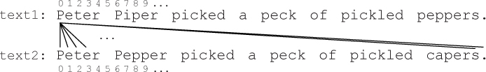
After we have compared text1[0] to all of the characters in text2, we need to repeat this process with text1[1], comparing text1[1] to text2[0], then text1[1] to text2[1], then text1[1] to text2[2], etc., as illustrated below:

In other words, for each value of index, we want to compare text1[index] to every base in text2, not just to text2[index]. To accomplish this, we need to replace the if statement in dotplot1 with another for loop:
import matplotlib.pyplot as pyplot

def dotplot(text1, text2):
    """Display a dot plot comparing two strings.

    Parameters:
        text1: a string object
        text2: a string object

    Return value: None
    """

    text1 = text1.lower()
    text2 = text2.lower()
    x = []
    y = []
    for index in range(len(text1)):
        for index2 in range(len(text2)):
            if text1[index] == text2[index2]:
                x.append(index)
                y.append(index2)
    pyplot.scatter(x, y)
    pyplot.xlim(0, len(text1))
    pyplot.ylim(0, len(text2))
    pyplot.xlabel(text1)
    pyplot.ylabel(text2)
    pyplot.show()
With this change inside the first for loop, each character text1[index] is compared to every character in text2, indexed by the index variable index2, just as in the illustrations above. If a match is found, we append index to the x list and index2 to the y list.
Reflection 6.47 Suppose we pass in 'plum' for text1 and 'pea' for text2. Write the sequence of comparisons that would be made in the body of the for loop. How many comparisons are there?
There are 4 ⋅ 3 = 12 total comparisons because each of the four characters in 'plum' is compared to each of the three characters in 'pea'. These twelve comparisons, in order, are:
 1.    text1[0]   ==   text2[0]   or   'p'   ==   'p'
 2.    text1[0]   ==   text2[1]   or   'p'   ==   'e'
 3.    text1[0]   ==   text2[2]   or   'p'   ==   'a'
 4.    text1[1]   ==   text2[0]   or   'l'   ==   'p'
 5.    text1[1]   ==   text2[1]   or   'l'   ==   'e'
 6.    text1[1]   ==   text2[2]   or   'l'   ==   'a'
 7.    text1[2]   ==   text2[0]   or   'u'   ==   'p'
 8.    text1[2]   ==   text2[1]   or   'u'   ==   'e'
 9.    text1[2]   ==   text2[2]   or   'u'   ==   'a'
10.    text1[3]   ==   text2[0]   or   'm'   ==   'p'
11.    text1[3]   ==   text2[1]   or   'm'   ==   'e'
12.    text1[3]   ==   text2[2]   or   'm'   ==   'a'

Notice that when index is 0, the inner for loop runs through all the values of index2. Then the inner loop finishes, also finishing the body of the outer for loop, and index is incremented to 1. The inner loop then runs through all of its values again, and so on.
Figure 6.6 shows the plot from the revised version of the function. Because the two strings share many characters, there are quite a few matches, contributing to a “noisy” plot. But the plot does now pick up the similarity in the strings, illustrated by the dots along the main diagonal.
We can reduce the “noise” in a dot plot by comparing substrings instead of individual characters. In textual analysis applications, substrings with length n are known as n-grams. When n > 1, there are many more possible substrings, so fewer matches tend to exist. Exercise 6.6.5 asks you to generalize this dot plot function so that it compares all n-grams in the two texts instead of all single characters. Figure 6.7 shows the result of this function with n = 3.
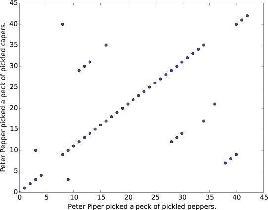
Figure 6.7 Output from the dotplot function from Exercise 6.6.5 (3-grams).
An interesting application of dot plots is in plagiarism detection. For example, Figure 6.8 shows a dot plot comparison between the following two passages. The first is from page 23 of The Age of Extremes: A History of the World, 1914–1991 by Eric Hobsbawm [19]:
All this changed in 1914. The First World War involved all major powers and indeed all European states except Spain, the Netherlands, the three Scandinavian countries and Switzerland. What is more, troops from the world overseas were, often for the first time, sent to fight and work outside their own regions.
The second is a fictitious attempt to plagiarize Hobsbawm’s passage:
All of this changed in 1914. World War I involved all major powers and all European states except the three Scandinavian countries, Spain, the Netherlands, and Switzerland. In addition, troops from the world overseas were sent to fight and work outside their own regions.
Reflection 6.48 Just by looking at Figure 6.8, would you conclude that the passage had been plagiarized? (Think about what a dotplot comparing two random passages would look like.)

Exercises
6.6.1. What is printed by the following nested loop?
text = 'imho'
for index1 in range(len(text)):
    for index2 in range(index1, len(text)):
        print(text[index1:index2 + 1])
6.6.2. Write a function
difference(word1, word2)
that returns the first index at which the strings word1 and word2 differ. If the words have different lengths, and the shorter word is a prefix of the longer word, the function should return the length of the shorter word. If the two words are the same, the function should return −1. Do this without directly testing whether word1 and word2 are equal.
6.6.3. Hamming distance, defined to be the number of bit positions that are different between two bit strings, is used to measure the error that is introduced when data is sent over a network. For example, suppose we sent the bit sequence 011100110001 over a network, but the destination received 011000110101 instead. To measure the transmission error, we can find the Hamming distance between the two sequences by lining them up as follows:
Sent: 011100110001
Received: 011000110101
Since the bit sequences are different in two positions, the Hamming distance is 2. Write a function
hamming(bits1, bits2)
that returns the Hamming distance between the two given bit strings. Assume that the two strings have the same length.
6.6.4. Repeat Exercise 6.6.3, but make it work correctly even if the two strings have different lengths. In this case, each “missing” bit at the end of the shorter string counts as one toward the Hamming distance. For example, hamming('000', '10011') should return 3.
6.6.5. Generalize the dotplot function so that it compares n-grams instead of individual characters.
6.6.6. One might be able to gain insight into a text by viewing the frequency with which a word appears in “windows” of some length over the length of the text. Consider the very small example below, in which we are counting the frequency of the “word” a in windows of size 4 in the string 'abracadabradab':

In this example, the window skips ahead 3 characters each time. So the four windows’ frequencies are 2, 2, 1, 2, which can be plotted like this:

The numbers on the x-axis are indices of the beginnings of each window. Write a function
wordFrequency(fileName, word, windowSize, skip)

that displays a plot like this showing the frequencies of the string word in windows of size windowSize, where the windows skip ahead by skip indices each time. The text to analyze should be read in from the file with the given fileName.
*6.7 GENOMICS
Every living cell contains molecules of DNA (deoxyribonucleic acid) that encode the genetic blueprint of the organism. Decoding the information contained in DNA, and understanding how it is used in all the processes of life, is an ongoing grand challenge at the center of modern biology and medicine. Comparing the DNA of different organisms also provides insight into evolution and the tree of life. The lengths of DNA molecules and the sheer quantity of DNA data that have been read from living cells and recorded in text files require that biologists use computational methods to answer this challenge.
A genomics primer
As illustrated in Figure 6.9, DNA is a long double-stranded molecule in the shape of a double helix. Each strand is a chain of smaller units called nucleotides. A nucleotide consists of a sugar (deoxyribose), a phosphate group, and one of four nitrogenous bases: adenine (A), thymine (T), cytosine (C), or guanine (G). Each nucleotide in a molecule can be represented by the letter corresponding to the base it contains, and an entire strand can be represented by a string of characters corresponding to its sequence of nucleotides. For example, the following string represents a small DNA molecule consisting of an adenine nucleotide followed by a guanine nucleotide followed by a cytosine nucleotide, etc.:
>>> dna = 'agcttttcattctgactg'
(The case of the characters is irrelevant; some sequence repositories use lower case and some use upper case.) Real DNA sequences are stored in large text files; we will look more closely at these later.
A base on one strand is connected via a hydrogen bond to a complementary base on the other strand. C and G are complements, as are A and T. A base and its connected complement are called a base pair. The two strands are “antiparallel” in the sense that they are traversed in opposite directions by the cellular machinery that copies and reads DNA. On each strand, DNA is read in an “upstream-to-downstream” direction, but the “upstream” and “downstream” ends are reversed on the two strands. For reasons that are not relevant here, the “upstream” end is called 5’ (read “five prime”) and the downstream end is called 3’ (read “three prime”). For example, the sequence in the top strand below, read from 5’ to 3’, is AGCTT...CTG, while the bottom strand, called its reverse complement, also read 5’ to 3’, is CAGTC...GCT.

Reflection 6.49 When DNA sequences are stored in text files, only the sequence on one strand is stored. Why?
RNA (ribonucleic acid) is a similar molecule, but each nucleotide contains a different sugar (ribose instead of deoxyribose), and a base named uracil (U) takes the place of thymine (T). RNA molecules are also single-stranded. As a result, RNA tends to “fold” when complementary bases on the same strand pair with each other. This folded structure forms a unique three-dimensional shape that plays a significant role in the molecule’s function.
Some regions of a DNA molecule are called genes because they encode genetic information. A gene is transcribed by an enzyme called RNA polymerase to produce a complementary molecule of RNA. For example, the DNA sequence 5'-GACTGAT-3' would be transcribed into the RNA sequence 3'-CUGACUA-5'. If the RNA is a messenger RNA (mRNA), then it contains a coding region that will ultimately be used to build a protein. Other RNA products of transcription, called RNA genes, are not translated into proteins, and are often instead involved in regulating whether genes are transcribed or translated into proteins. Upstream from the transcribed sequence is a promoter region that binds to RNA polymerase to initiate transcription. Upstream from there is often a regulatory region that influences whether or not the gene is transcribed.

Table 6.1 The standard genetic code that translates between codons and amino acids. For each codon, both the three letter code and the single letter code are shown for the corresponding amino acid.

The coding region of a mRNA is translated into a protein by a molecular machine called a ribosome. A ribosome reads the coding region in groups of three nucleotides called codons. In prokaryotes (e.g., bacteria), the coding region begins with a particular start codon and ends with one of three stop codons. The ribosome translates each mRNA codon between the start and stop codons into an amino acid, according to the genetic code, shown in Table 6.1. It is this sequence of amino acids that comprises the final protein. The genes of eukaryotes (organisms whose cells contain a nucleus) are more complicated, partially because they are interspersed with untranslated regions called introns that must be spliced out before translation can occur.
Reflection 6.50 What amino acid sequence is represented by the mRNA sequence CAU UUU GAG?
Reflection 6.51 Notice that, in the genetic code (Table 6.1), most amino acids are represented by several similar codons. Keeping in mind that nucleotides can mutate over time, what evolutionary advantage might this hold?
The complete sequence of an organism’s DNA is called its genome. The size of a genome can range from 105 base pairs (bp) in the simplest bacteria to 1.5 × 10¹¹ bp in some plants. The human genome contains about 3.2 × 10⁹ (3.2 billion) bp. Interestingly, the size of an organism’s genome does not necessarily correspond to its complexity; plants have some of the largest genomes, far exceeding the size of the human genome.
The subfield of biology that studies the structure and function of genomes is called genomics. To better understand a genome, genomicists ask questions such as:
What is the frequency of each base in the genome? What is the frequency of each codon? For each amino acid, is there a bias toward particular codons?
Where are the genes and what are their functions?
How similar are two sequences? Sequence comparison can be used to determine whether two genes have a shared ancestry, called homology. Sequence comparison between homologous sequences can also give clues to an unidentified gene’s function.
How are a set of organisms related evolutionarily? We can use sequence comparison to build a phylogenetic tree that specifies genetic relations between species.
Scientists have discovered that mammalian genomes are largely reshuffled collections of similar blocks, called synteny blocks. What is the most likely sequence of rearrangement events to have changed one genome into the other?
What genes are regulated together? Identifying groups of genes that are regulated in the same way can lead to insights into genes’ functions, especially those related to disease.
Because genomes are so large, questions like these can only be answered computationally. In the next few pages, we will look at how the methods and techniques from previous sections can be used to answer some of the questions above. We leave many additional examples as exercises. We will begin by working with small sequences; later, we will discuss how to read some longer sequences from files and the web.
Basic DNA analysis
We can use some of the techniques from the previous section to answer questions in the first bullet above. For example, bacterial genomes are sometimes categorized according to their ratio of G and C bases to A and T bases. The fraction of bases that are G or C is called the genome’s GC content. There are a few ways that we can compute the GC content. First, we could simply use the count method:
>>> gc = (dna.count('c') + dna.count('g')) / len(dna)
>>> gc
0.3888888888888889
Or, we could use a for loop like the count1 function in the previous section:
def gcContent(dna):
    """Compute the GC content of a DNA sequence.

    Parameter:
        dna: a string representing a DNA sequence

    Return value: the GC content of the DNA sequence
    """

    dna = dna.lower()
    count = 0
    for nt in dna:                 # nt is short for "nucleotide"
        if nt in 'cg':
            count = count + 1
    return count / len(dna)
Reflection 6.52 Why do we convert dna to lower case at the beginning of the function?
Because DNA sequences can be in either upper or lower case, we need to account for both possibilities when we write a function. But rather than check for both possibilities in our functions, it is easier to just convert the parameter to either upper or lower case at the beginning.
To gather statistics about the codons in genes, we need to count the number of non-overlapping occurrences of any particular codon. This is very similar to the count function from the previous section, except that we need to increment the index variable by three in each step:
def countCodon(dna, codon):
    """Find the number of occurrences of a codon in a DNA sequence.

    Parameters:
        dna: a string representing a DNA sequence
        codon: a string representing a codon

    Return value: the number of occurrences of the codon in dna
    """

    count = 0
    for index in range(0, len(dna) - 2, 3):
        if dna[index:index + 3] == codon:
            count = count + 1
    return count
Reflection 6.53 Why do we subtract 2 from len(dna) above?
Transforming sequences
When DNA sequences are stored in databases, only the sequence of one strand is stored. But genes and other features may exist on either strand, so we need to be able to derive the reverse complement sequence from the original. To first compute the complement of a sequence, we can use a string accumulator, but append the complement of each base in each iteration.
def complement(dna):
    """Return the complement of a DNA sequence.

    Parameter:
        dna: a string representing a DNA sequence

    Return value: the complement of the DNA sequence
    """

    dna = dna.lower()
    compdna = ''
    for nt in dna:
        if nt == 'a':
            compdna = compdna   + 't'
        elif nt == 'c':
            compdna = compdna   + 'g'
        elif nt == 'g':
            compdna = compdna   + 'c'
        else:
            compdna = compdna   + 'a'
    return compdna
To turn our complement into a reverse complement, we need to write an algorithm to reverse a string of DNA. Let’s look at two different ways we might do this. First, we could iterate over the original string in reverse order and append the characters to the new string in that order.
Reflection 6.54 How can we iterate over indices in reverse order?
We can iterate over the indices in reverse order by using a range that starts at len(dna) - 1 and goes down to, but not including, −1 using a step of −1. A function that uses this technique follows.
def reverse(dna):
    """Return the reverse of a DNA sequence.

     Parameter:
         dna: a string representing a DNA sequence

     Return value: the reverse of the DNA sequence
     """

     revdna = ''
     for index in range(len(dna) - 1, -1, -1):
         revdna = revdna + dna[index]
     return revdna
A more elegant solution simply iterates over the characters in dna in the normal order, but prepends each character to the revdna string.
def reverse(dna):
    """ (docstring omitted) """

     revdna = ''
     for nt in dna:
         revdna = nt + revdna
     return revdna
To see how this works, suppose dna was 'agct'. The table below illustrates how each value changes in each iteration of the loop.
| Iteration | nt |
new value of revdna |
1 |
'a' |
'a' + '' → 'a' |
2 |
'g' |
'g' + 'a' → 'ga' |
3 |
'c' |
'c' + 'ga' → 'cga' |
4 |
't' |
't' + 'cga' → 'tcga' |
Finally, we can put these two pieces together to create a function for reverse complement:
def reverseComplement(dna):
    """Return the reverse complement of a DNA sequence.

    Parameter:
        dna: a string representing a DNA sequence

    Return value: the reverse complement of the DNA sequence
    """

    return reverse(complement(dna))
This function first computes the complement of dna, then calls reverse on the result. We can now, for example, use the reverseComplement function to count the frequency of a particular codon on both strands of a DNA sequence:
countForward = countCodon(dna, 'atg')
countBackward = countCodon(reverseComplement(dna), 'atg')
Comparing sequences
Measuring the similarity between DNA sequences, called comparative genomics, has become an important area in modern biology. Comparing the genomes of different species can provide fundamental insights into evolutionary relationships. Biologists can also discover the function of an unknown gene by comparing it to genes with known functions in evolutionarily related species.
Dot plots are used heavily in computational genomics to provide visual representations of how similar large DNA and amino sequences are. Consider the following two sequences. The dotplot1 function in Section 6.5 would show pairwise matches between the nucleotides in black only.
Sequence 1: |
|
Sequence 2: |
|
But notice that the last four bases in the two sequences are actually the same; if you insert a gap in the first sequence, above the last T in the second sequence, then the number of differing bases drops from eight to four, as illustrated below.
Sequence 1: |
|
Sequence 2: |
|
Evolutionarily, if the DNA of the closest common ancestor of these two species contained a T in the location of the gap, then we interpret the gap as a deletion in the first sequence. Or, if the closest common ancestor did not have this T, then we interpret the gap as an insertion in the second sequence. These insertions and deletions, collectively called indels, are common; therefore, sequence comparison algorithms must take them into account. So, just as the first dotplot1 function did not adequately represent the similarity between texts, neither does it for DNA sequences. Figure 6.10 shows a complete dot plot, using the dotplot function from Section 6.5, for the sequences above.
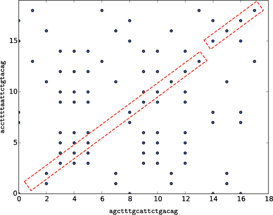
Figure 6.10 A dot plot comparing individual bases in agctttgcattctgacag and accttttaattctgtacag. The dots representing the main alignment are highlighted.
As we saw in the previous section, dot plots tend to be more useful when we reduce the “noise” by instead comparing subsequences of a given length, say ℓ, within a sliding window. Because there are 4ℓ different possible subsequences with length ℓ, fewer matches are likely. Dot plots are also more useful when comparing sequences of amino acids. Since there are 20 different amino acids, we tend to see less noise in the plots. For example, Figure 6.11 shows a dot plot for the following hypothetical small proteins. Each letter corresponds to a different amino acid. (See Table 6.1 for the meanings of the letters if you are interested.)
seq1 = 'PDAQNPDMSFFKMLFLPESARWIQRTHGKNS'
seq2 = 'PDAQNPDMPLFLMKFFSESARWIQRTHGKNS'
Notice how the plot shows an inversion in one sequence compared the other, highlighted in red above.
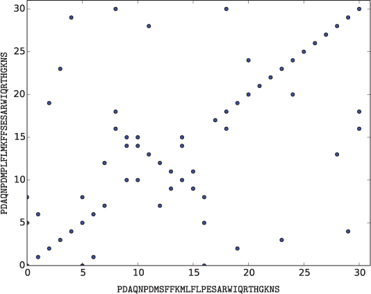
Reading sequence files
DNA sequences are archived and made publicly available in a database managed by the National Center for Biotechnology Information (NCBI), a division of the National Institutes of Health (NIH). Each sequence in the database has an associated identifier known as an accession number. For example, the accession number for the first segment of the Burmese python (Python molurus bivittatus) genome is AEQU02000001. You can find this data by visiting the NCBI web site at http://www.ncbi.nlm.nih.gov, entering the accession number in the search box, and selecting “Nucleotide” from the drop-down menu.
Genomic data is commonly stored in a format called FASTA [38]. A FASTA file begins with a header preceded by a greater-than sign (>), followed by several lines of sequence data. Each line of sequence is terminated with a newline character. For example, the FASTA file for the first segment of the Burmese python genome looks like this:
>gi|541020484|gb|AEQU02000001.1| Python bivittatus ...
AGGCCTGGCGCAATATGGTTCATGGGGTCACGAAGAGTCGGACACGACTTAACGACTAAACAACAATTAA
TTCTAAACCCTAGCTATCTGGGTTGCTTCCCTACATTATATTTCCGTGAATAAATCTCACTAAACTCAGA
AGGATTTACTTTTGAGTGAACACTCATGATCAAGAACTCAGAAAACTGAAAGGATTCGGGAATAGAAGTG
TTATTTCAGCCCTTTCCAATCTTCTAAAAAGCTGACAGTAATACCTTTTTTTGTTTTAAAAATTTAAAAA
GAGCACTCACATTTATGCTACAGAATGAGTCTGTAACAGGGAAGCCAGAAGGGAAAAAGACTGAAACGTA
AACCAAGGACATAATGCAGGGATCATAATTTCTAGTTGGCAAGACTAAAGTCTATACATGTTTTATTGAA
AAACCACTGCTATTTGCTCTTACAAGAACTTATCCCTCCAGAAAAAGTAGCACTGGCTTGATACTGCCTG
CTCTAACTCAACAGTTTCAGGAAGTGCTGGCAGCCCCTCCTAACACCATCTCAGCTAGCAAGACCAAGTT
GTGCAAGTCCACTCTATCTCATAACAAAACCTCTTTAATTAAACTTGAAAGCCTAGAGCTTTTTTTACCT
TGGTTCTTCAAGTCTTCGTTTGTACAATATGGGCCAATGTCATAGCTTGGTGTATTAGTATTATTATTGT
TACTGTTGGTTACACAGTCAGTCAGATGTTTAGACTGGATTTGACATTTTTACCCATGTATCGAGTCCTT
CCCAAGGACCTGGGATAGGCAGATGTTGGTGTTTGATGGTGTTAAAGGT
To use this DNA sequence in a program, we need to extract the unadorned sequence into a string, removing the header and newline characters. A function to do this is very similar to those in Section 6.2.
def readFASTA(filename):
    """Read a FASTA file containing a single sequence and return
       the sequence as a string.

     Parameter:
         filename: a string representing the name of a FASTA file

     Return value: a string containing the sequence in the FASTA file
     """

     inputFile = open(filename, 'r', encoding = 'utf-8')
     header = inputFile.readline()
     dna = ''
     for line in inputFile:
         dna = dna + line[:-1]
     inputFile.close()
     return dna
After opening the FASTA file, we read the header line with the readline function. We will not need this header, so this readline just serves to move the file pointer past the first line, to the start of the actual sequence. To read the rest of the file, we iterate over it, line by line. In each iteration, we append the line, without the newline character at the end, to a growing string named dna. There is a link on the book website to the FASTA file above so that you can try out this function.
We can also directly access FASTA files by using a URL that sends a query to NCBI. The URL below submits a request to the NCBI web site to download the FASTA file for the first segment of the Burmese python genome (with accession number AEQU02000001).
http://eutils.ncbi.nlm.nih.gov/entrez/eutils/efetch.fcgi?db=nuccore
   &id=AEQU02000001&rettype=fasta&retmode=text
To retrieve a different sequence, we would just need to insert a different accession number (in red). The following function puts all of the pieces together.
import urllib.request as web

def getFASTA(id):
    """Fetch the DNA sequence with the given id from NCBI and return
       it as a string.

    Parameter:
        id: the identifier of a DNA sequence

    Return value: a string representing the sequence with the given id
    """

    prefix1 = 'http://eutils.ncbi.nlm.nih.gov/entrez/eutils/efetch.fcgi'
    prefix2 = '?db=nuccore&id='
    suffix = '&rettype=fasta&retmode=text'
    url = prefix1 + prefix2 + id + suffix
    readFile = web.urlopen(url)
    header = readFile.readline()
    dna = ''
    for line in readFile:
        line = line[:-1]
        dna = dna + line.decode('utf-8')
    readFile.close()
    return dna
The function first creates a string containing the URL for the accession number passed in parameter id. The first common parts of the URL are assigned to the prefix variables, and the last part of the URL is assigned to suffix. We construct the custom URL by concatenating these pieces with the accession number. We then open the URL and use the code from the previous readFASTA function to extract the DNA sequence and return it as a string.
Reflection 6.55 Use the getFASTA function to read the first segment of the Burmese python genome (accession number AEQU02000001).
We have just barely touched on the growing field of computational genomics. The following exercises explore some additional problems and provide many opportunities to practice your algorithm design and programming skills.
Exercises
6.7.1. Write a function
countACG(dna)
that returns the fraction of nucleotides in the given DNA sequence that are not T. Use a for loop that iterates over the characters in the string.
6.7.2. Repeat the previous exercise, but use a for loop that iterates over the indices of the string instead.
printCodons(dna)
that prints the codons, starting at the left end, in the string dna. For example, printCodons('ggtacactgt') would print
ggt
aca
ctg
6.7.4. Write a function
findCodon(dna, codon)
that returns the index of the first occurrence of the given codon in the string dna. Unlike in the countCodon function, increment the loop index by 1 instead of 3, so you can find the codon at any position.
6.7.5. Write a function
findATG(dna)
that builds up a list of indices of all of the positions of the codon ATG in the given DNA string. Do not use the built-in index method or find method. Constructing the list of indices is very similar to what we have done several times in building lists to plot.
6.7.6. Since codons consist of three bases each, transcription can occur in one of three independent reading frames in any sequence of DNA by starting at offsets 0, 1, and 2 from the left end. For example, if our DNA sequence was ggtacactgtcat, the codons in the three reading frames are:
RF 1: |
|
RF 2: |
|
RF 3: |
|
Write a function
printCodonsAll(dna)
that uses your function from Exercise 6.7.3 to print the codons in all three reading frames.
6.7.7. Most vertebrates have much lower density of CG pairs (called CG dinucleotides) than would be expected by chance. However, they often have relatively high concentrations upstream from genes (coding regions). For this reason, finding these so-called “CpG islands” is often a good way to find putative sites of genes. (The “p” between C and G denotes the phosphodiester bond between the C and G, versus a hydrogen bond across two complementary strands.) Without using the built-in count method, write a function
CpG(dna)
that returns the fraction of dinucleotides that are cg. For example, if dna were atcgttcg, then the function should return 0.5 because half of the sequence is composed of CG dinucleotides.
6.7.8. A microsatellite or simple sequence repeat (SSR) is a repeat of a short sequence of DNA. The repeated sequence is typically 2–4 bases in length and can be repeated 10–100 times or more. For example, cacacacaca is a short SSR of ca, a very common repeat in humans. Microsatellites are very common in the DNA of most organisms, but their lengths are highly variable within populations because of replication errors resulting from “slippage” during copying. Comparing the distribution of length variants within and between populations can be used to determine genetic relationships and learn about evolutionary processes.
Write a function
ssr(dna, repeat)
that returns the length (number of repeats) of the first SSR in dna that repeats the parameter repeat. If repeat is not found, return 0. Use the find method of the string class to find the first instance of repeat in dna.
6.7.9. Write another version of the ssr function that finds the length of the longest SSR in dna that repeats the parameter repeat. Your function should repeatedly call the ssr function in the previous problem. You will probably want to use a while loop.
6.7.10. Write a third version of the ssr function that uses the function in the previous problem to find the longest SSR of any dinucleotide (sequence with length 2) in dna. Your function should return the longest repeated dinucleotide.
6.7.11. Write a function
palindrome(dna)
that returns True if dna is the same as its reverse complement, and False otherwise. (Note that this is different from the standard definition of palindrome.) For example, gaattc is a palindrome because it and its reverse complement are the same. These sequences turn out to be very important because certain restriction enzymes target specific palindromic sequences and cut the DNA molecule at that location. For example, the EcoR1 restriction enzyme cuts DNA of the bacteria Escherichia coli at the sequence gaattc in the following way:
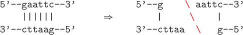
6.7.12. Write a function
dna2rna(dna)
that returns returns a copy of dna with every T replaced by a U.
6.7.13. Write a function
transcribe(dna)
that returns the RNA equivalent of the reverse complement of dna. (Utilize previously written functions to accomplish this in one line.)
6.7.14. Write a function
clean(dna)
that returns a new DNA string in which every character that is not an A, C, G, or T is replaced with an N. For example, clean('goat') should return the string 'gnat'.
6.7.15. When DNA molecules are sequenced, there are often ambiguities that arise in the process. To handle these situations, there are also “ambiguous symbols” defined that code for one of a set of bases.
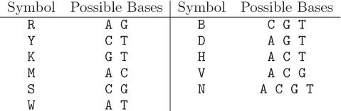
Write a function
fix(dna)
that returns a DNA string in which each ambiguous symbol is replaced with one of the possible bases it represents, each with equal probability. For example, if an R exists in dna, it should be replaced with either an A with probability 1/2 or a G with probability 1/2.
6.7.16. Write a function
mark(dna)
that returns a new DNA string in which every start codon ATG is replaced with >>>, and every stop codon (TAA, TAG, or TGA) is replaced with <<<. Your loop should increment by 3 in each iteration so that you are only considering non-overlapping codons. For example, mark('ttgatggagcattagaag') should return the string 'ttg>>>gagcat<<<aag'.
6.7.17. The accession number for the hepatitis A virus is NC_001489. Write a program that uses the getFASTA function to get the DNA sequence for hepatitis A, and then the gcContent function from this section to find the GC content of hepatitis A.
6.7.18. The DNA of the hepatitis C virus encodes a single long protein that is eventually processed by enzymes called proteases to produce ten smaller proteins. There are seven different types of the virus. The accession numbers for the proteins produced by type 1 and type 2 are NP_671491 and YP_001469630. Write a program that uses the getFASTA function and your dot plot function from Exercise 6.6.5 to produce a dot plot comparing these two proteins using a window of size 4.
6.7.19. Hox genes control key aspects of embryonic development. Early in development, the embryo consists of several segments that will eventually become the main axis of the head-to-tail body plan. The Hox genes dictate what body part each segment will become. One particular Hox gene, called Hox A1, seems to control development of the hindbrain. Write a program that uses the getFASTA function and your dot plot function from Exercise 6.6.5 to produce a dot plot comparing the human and mouse Hox A1 genes, using a window of size 8. The human Hox A1 gene has accession number U10421.1 and the mouse Hox A1 gene has accession number NM_010449.4.
6.8 SUMMARY
Text is stored as a sequence of bytes, which we can read into one or more strings. The most fundamental string algorithms have one of the following structures:
for character in text:
    # process character

for index in range(len(text)):
    # process text[index]
In the first case, consecutive characters in the string are assigned to the for loop index variable character. In the body of the loop, each character can then be examined individually. In the second case, consecutive integers from the list [0, 1, 2, ..., len(text) - 1], which are precisely the indices of the characters in the string, are assigned to the for loop index variable index. In this case, the algorithm has more information because, not only can it access the character at text[index], it also knows where that character resides in the string. The first choice tends to be more elegant, but the second choice is necessary when the algorithm needs to know the index of each character, or if it needs to process slices of the string, which can only be accessed with indices.
We called one special case of these loops a string accumulator:
newText = ''
for character in text:
    newText = newText + _______
Like an integer accumulator and a list accumulator, a string accumulator builds its result cumulatively in each iteration of the loop. Because strings are immutable, a string accumulator must create a new string in each iteration that is composed of the old string with a new character concatenated.
Algorithms like these that perform one pass over their string parameters and execute a constant number of elementary steps per character are called linear-time algorithms because their number of elementary steps is proportional to the length of the input string.
In some cases, we need to compare every character in one string to every character in a second string, so we need a nested loop like the following:
for index1 in range(len(text1)):
    for index2 in range(len(text2)):
        # process text1[index1] and text2[index2]
If both strings have length n, then a nested loop like this constitutes a quadratic-time algorithm with time complexity n2 (as long as the body of the loop is constant-time) because every one of n characters in the first string is compared to every one of n characters in the second string. We will see more loops like this in later chapters.
6.9 FURTHER DISCOVERY
The first of the two epigraphs at the beginning of this chapter is from the following blog post by Leslie Johnston, the former Chief of the Repository Development Center at the Library of Congress. She is currently Director of Digital Preservation at The National Archives.
http://blogs.loc.gov/digitalpreservation/2012/04/
a-library-of-congress-worth-of-data-its-all-in-how-you-define-it/
The second epigraph is from an article titled “The DNA Data Deluge” by Michael C. Schatz and Ben Langmead [46], which can be found at
http://spectrum.ieee.org/biomedical/devices/the-dna-data-deluge.
The Keyword in Context (KWIC) indexing system, also known as a permuted index, is similar to a concordance. In a KWIC index, every word in the title of an article appears in the index in the context in which it appears.
If you are interested in learning more about computational biology, two good places to start are The Mathematics of Life [53] by Ian Stewart and Natural Computing [51] by Dennis Shasha and Cathy Lazere. The latter book has a wider focus than just computational biology.
6.10 PROJECTS
Project 6.1 Polarized politics
The legislative branch of the United States government, with its two-party system, goes through phases in which the two parties work together productively to pass laws, and other phases in which partisan lawmaking is closer to the norm. In this project, we will use data available on the website of the Clerk of the U.S. House of Representatives (http://clerk.house.gov/legislative/legvotes.aspx) to analyze the voting behavior and polarization of the U.S. House over time.
Part 1: Party line votes
We will call a vote party line when at least half of the voting members of one party vote one way and at least half of the voting members of the other party vote the other way. In the House, when the vote of every member is recorded, it is called a roll call vote. Individual roll call votes are available online at URLs that look like the following:
http://clerk.house.gov/evs/<year>/roll<number>.xml
The placeholder <year> is replaced with the year of the vote and the placeholder <number> is replaced with the roll call number. For example, the results of roll call vote 194 from 2010 (the final vote on the Affordable Care Act) are available at
http://clerk.house.gov/evs/2010/roll194.xml
If the roll call number has fewer than three digits, the number is filled with zeros. For example, the results of roll call vote 11 from 2010 are available at
http://clerk.house.gov/evs/2010/roll011.xml
Run the following program to view one of these files:
import urllib.request as web

def main():
    url = 'http://clerk.house.gov/evs/2010/roll194.xml'
    webpage = web.urlopen(url)
    for line in webpage:
        line = line.decode('utf-8')
        print(line.rstrip())
    webpage.close()

main()
You will notice many XML elements contained in matching
<recorded-vote> ... </recorded-vote>
tags. Each of these elements is a vote of one member of the House.
To begin, write a function
partyLine(year, number)
that determines whether House roll call vote number from the given year was a party line vote. Use only the recorded vote elements, and no other parts of the XML files. Do not use any built-in string methods. Be aware that some votes are recorded as Yea/Nay and some are recorded as Aye/No. Do not count votes that are recorded in any other way (e.g., “Present” or “Not Voting”), even toward the total numbers of votes. Test your function thoroughly before moving to the next step.
Question 6.1.1 What type of data should this function return? (Think about making your life easier for the next function.)
Question 6.1.2 Was the vote on the Affordable Care Act a party line vote?
Question 6.1.3 Choose another vote that you care about. Was it a party line vote?
Second, write another function
countPartyLine(year, maxNumber)
that uses the partyLine function to return the fraction of votes that were party line votes during the given year. The parameter maxNumber is the number of the last roll call vote of the year.
Finally, write a function
plotPartyLine()
that plots the fractions of party line votes for the last 20 years. To keep things simple, you may assume that there were 450 roll call votes each year. If you would prefer to count all of the roll call votes, here are the numbers for each of the last 20 years:

Question 6.1.4 What fraction of votes from each of years 1994 to 2013 went along party lines?
Note that collecting this data may take a long time, so make sure that your functions are correct for a single year first.
Question 6.1.5 Describe your plot. Has American politics become more polarized over the last 20 years?
Question 6.1.6 Many news outlets report on the issue of polarization. Find a news story about this topic online, and compare your results to the story. It might be helpful to think about the motivations of news outlets.
Part 2: Blue state, red state
We can use the roll call vote files to infer other statistics as well. For this part, write a function
stateDivide(state)
that plots the number of Democratic and Republican representatives for the given state every year for the last 20 years. Your plot should have two different curves (one for Democrat and one for Republican). You may also include curves for other political parties if you would like. Test your function on several different states.
Call your stateDivide function for at least five states, including your home state.
Question 6.1.7 Describe the curves you get for each state. Interpret your results in light of the results from Part 1. Has the House of Representatives become more polarized?
*Project 6.2 Finding genes
This project assumes that you have read Section 6.7.
In prokaryotic organisms, the coding regions of genes are usually preceded by the start codon ATG, and terminated by one of three stop codons, TAA, TAG, and TGA. A long region of DNA that is framed by start and stop codons, with no stop codons in between, is called an open reading frame (or ORF). Searching for sufficiently long ORFs is an effective (but not fool-proof) way to locate putative genes.
For example, the rectangle below marks a particular open reading frame beginning with the start codon ATG and ending with the stop codon TAA. Notice that there are no other stop codons in between.
![]()
Not every ORF corresponds to a gene. Since there are 43 = 64 possible codons and 3 different stop codons, one is likely to find a stop codon approximately every 64/3 ≈ 21 codons in a random stretch of DNA. Therefore, we are really only interested in ORFs that have lengths substantially longer than this. Since such long ORFs are unlikely to occur by chance, there is good reason to believe that they may represent a coding region of a gene.
Not all open reading frames on a strand of DNA will be aligned with the left (5’) end of the sequence. For instance, in the example above, if we only started searching for open reading frames in the codons aligned with the left end — ggc, gga, tga, etc. — we would have missed the boxed open reading frame. To find all open reading frames in a strand of DNA, we must look at the codon sequences with offsets 0, 1, and 2 from the left end. (See Exercise 6.7.6 for another example.) The codon sequences with these offsets are known as the three forward reading frames. In the example above, the three forward reading frames begin as follows:
| Reading frame 0: | ggc gga tga aac ... |
Reading frame 1: |
|
Reading frame 2: |
|
Because DNA is double stranded, with a reverse complement sequence on the other strand, there are also three reverse reading frames. In this strand of DNA, the reverse reading frames would be:
Reverse reading frame 0: |
|
Reverse reading frame 1: |
|
Reverse reading frame 2: |
|
Because genomic sequences are so long, finding ORFs must be performed computationally. For example, consider the following sequence of 1,260 nucleotides from an Escherichia coli (or E. coli) genome, representing only about 0.03% of the complete genome. (This number represents about 0.00005% of the human genome.) Can you find an open reading frame in this sequence?
agcttttcattctgactgcaacgggcaatatgtctctgtgtggattaaaaaaagagtgtctgatagcagc
ttctgaactggttacctgccgtgagtaaattaaaattttattgacttaggtcactaaatactttaaccaa
tataggcatagcgcacagacagataaaaattacagagtacacaacatccatgaaacgcattagcaccacc
attaccaccaccatcaccattaccacaggtaacggtgcgggctgacgcgtacaggaaacacagaaaaaag
cccgcacctgacagtgcgggcttttttttcgaccaaaggtaacgaggtaacaaccatgcgagtgttgaag
ttcggcggtacatcagtggcaaatgcagaacgttttctgcgggttgccgatattctggaaagcaatgcca
ggcaggggcaggtggccaccgtcctctctgcccccgccaaaatcaccaaccatctggtagcgatgattga
aaaaaccattagcggtcaggatgctttacccaatatcagcgatgccgaacgtatttttgccgaacttctg
acgggactcgccgccgcccagccgggatttccgctggcacaattgaaaactttcgtcgaccaggaatttg
cccaaataaaacatgtcctgcatggcatcagtttgttggggcagtgcccggatagcatcaacgctgcgct
gatttgccgtggcgagaaaatgtcgatcgccattatggccggcgtgttagaagcgcgtggtcacaacgtt
accgttatcgatccggtcgaaaaactgctggcagtgggtcattacctcgaatctaccgttgatattgctg
aatccacccgccgtattgcggcaagccgcattccggctgaccacatggtgctgatggctggtttcactgc
cggtaatgaaaaaggcgagctggtggttctgggacgcaacggttccgactactccgctgcggtgctggcg
gcctgtttacgcgccgattgttgcgagatctggacggatgttgacggtgtttatacctgcgatccgcgtc
aggtgcccgatgcgaggttgttgaagtcgatgtcctatcaggaagcgatggagctttcttacttcggcgc
taaagttcttcacccccgcaccattacccccatcgcccagttccagatcccttgcctgattaaaaatacc
ggaaatccccaagcaccaggtacgctcattggtgccagccgtgatgaagacgaattaccggtcaagggca
This is clearly not a job for human beings. But, if you spent enough time, you might spot an ORF in reading frame 2 between positions 29 and 97, an ORF in reading frame 0 between positions 189 and 254, and another ORF in reading frame 0 between positions 915 and 1073 (to name just a few). These are highlighted in red below.
agcttttcattctgactgcaacgggcaatATGTCTCTGTGTGGATTAAAAAAAGAGTGTCTGATAGCAGC
TTCTGAACTGGTTACCTGCCGTGAGTAAattaaaattttattgacttaggtcactaaatactttaaccaa
tataggcatagcgcacagacagataaaaattacagagtacacaacatccATGAAACGCATTAGCACCACC
ATTACCACCACCATCACCATTACCACAGGTAACGGTGCGGGCTGAcgcgtacaggaaacacagaaaaaag
cccgcacctgacagtgcgggcttttttttcgaccaaaggtaacgaggtaacaaccatgcgagtgttgaag
ttcggcggtacatcagtggcaaatgcagaacgttttctgcgggttgccgatattctggaaagcaatgcca
ggcaggggcaggtggccaccgtcctctctgcccccgccaaaatcaccaaccatctggtagcgatgattga
aaaaaccattagcggtcaggatgctttacccaatatcagcgatgccgaacgtatttttgccgaacttctg
acgggactcgccgccgcccagccgggatttccgctggcacaattgaaaactttcgtcgaccaggaatttg
cccaaataaaacatgtcctgcatggcatcagtttgttggggcagtgcccggatagcatcaacgctgcgct
gatttgccgtggcgagaaaatgtcgatcgccattatggccggcgtgttagaagcgcgtggtcacaacgtt
accgttatcgatccggtcgaaaaactgctggcagtgggtcattacctcgaatctaccgttgatattgctg
aatccacccgccgtattgcggcaagccgcattccggctgaccacatggtgctgatggctggtttcactgc
cggtaATGAAAAAGGCGAGCTGGTGGTTCTGGGACGCAACGGTTCCGACTACTCCGCTGCGGTGCTGGCG
GCCTGTTTACGCGCCGATTGTTGCGAGATCTGGACGGATGTTGACGGTGTTTATACCTGCGATCCGCGTC
AGGTGCCCGATGCGAGGTTGTTGAagtcgatgtcctatcaggaagcgatggagctttcttacttcggcgc
taaagttcttcacccccgcaccattacccccatcgcccagttccagatcccttgcctgattaaaaatacc
ggaaatccccaagcaccaggtacgctcattggtgccagccgtgatgaagacgaattaccggtcaagggca
Of these three, only the second is actually a known gene.
Part 1: Find ORFs
For the first part of this project, we will read a text file containing a long DNA sequence, write this sequence to a turtle graphics window, and then draw bars with intervals of alternating colors over the sequence to indicate the locations of open reading frames. In the image below, which represents just a portion of a window, the three bars represent the three forward reading frames with reading frame 0 at the bottom. Look closely to see how the blue bars begin and end on start and stop codons (except for the top bar which ends further to the right). The two shorter blue bars are actually unlikely to be real genes due to their short length.
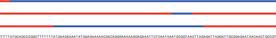
To help you get started and organize your project, you can download a “skeleton” of the program from the book web page. In the program, the viewer function sets up the turtle graphics window, writes the DNA sequence at the bottom (one character per x coordinate), and then calls the two functions that you will write. The main function reads a long DNA sequence from a file and into a string variable, and then calls viewer.
To display the open reading frames, you will write the function
orf1(dna, rf, tortoise)
to draw colored bars representing open reading frames in one forward reading frame with offset rf (0, 1, or 2) of string dna using the turtle named tortoise. This function will be called three times with different values of rf to draw the three reading frames. As explained in the skeleton program, the drawing function is already written; you just have to change colors at the appropriate times before calling it. Hint: Use a Boolean variable inORF in your for loop to keep track of whether you are currently in an ORF.
Also on the book site are files containing various size prefixes of the genome of a particular strain of E. coli. Start with the smaller files.
Question 6.2.1 How long do you think an open reading frame should be for us to consider it a likely gene?
Question 6.2.2 Where are the likely genes in the first 10,000 bases of the E. coli genome?
Part 2: GC content
The GC content of a particular stretch of DNA is the ratio of the number of C and G bases to the total number of bases. For example, in the following sequence
TCTACGACGT
the GC content is 0.5 because 5/10 of the bases are either C or G. Because the GC content is usually higher around coding sequences, this can also give clues about gene location. (This is actually more true in vertebrates than in bacteria like E. coli.) In long sequences, GC content can be measured over “windows” of a fixed size, as in the example we discussed back in Section 1.3. For example, in the tiny example above, if we measure GC content over windows of size 4, the resulting ratios are
TCTACGACGT

TCTA             0.25
 CTAC            0.50
  TACG           0.50
   ACGA          0.50
     CGAC        0.75
      GACG       0.75
       ACGT      0.50
We can then plot this like so:
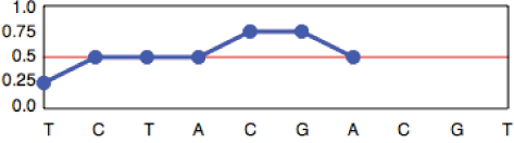

Finish writing the function
gcFreq(dna, window, tortoise)
that plots the GC frequency of the string dna over windows of size window using the turtle named tortoise. Plot this in the same window as the ORF bars. As explained in the skeleton code, the plotting function is already written; you just need to compute the correct GC fractions. As we discussed in Section 1.3, you should not need to count the GC content anew for each window. Once you have counted the G and C bases for the first window, you can incrementally modify this count for the subsequent windows. The final display should look something like Figure 6.12.
1See Appendix B.6 for a list.
2This file can be obtained from the book’s website or from Project Gutenberg at http://www.gutenberg.org/files/2701/2701.txt
3ASCII is an acronym for American Standard Code for Information Interchange.
4“Diligence is the mother of good luck.” is from The Way to Wealth (1758) by Benjamin Franklin.