
CHAPTER 9
Flatland
Suffice it that I am the completion of your incomplete self. You are a Line, but I am a Line of Lines, called in my country a Square: and even I, infinitely superior though I am to you, am of little account among the great nobles of Flatland, whence I have come to visit you, in the hope of enlightening your ignorance.
Edwin A. Abbott
Flatland: A Romance of Many Dimensions (1884)
THE title of this chapter is a reference to the highly-recommended book of the same name written by Edwin A. Abbott in 1884 [1]. In it, the narrator, a square who lives in the two-dimensional world of Flatland, discovers and grapples with comprehending the three-dimensional world of Spaceland, while simultaneously recognizing the profound advantages he has over those living in the zero- and one-dimensional worlds of Pointland and Lineland.
Analogously, we have discovered the advantages of one-dimensional data (strings and lists) over zero-dimensional numbers and characters. In this chapter, we will discover the further possibilities afforded us by understanding how to work with two-dimensional data. We will begin by looking at how we can create a two-dimensional table of data read in from a file. Then we will explore a powerful two-dimensional simulation technique called cellular automata. At the end of the chapter are several projects that illustrate how simulations similar to cellular automata can be used to model a wide variety of problems. We also spend some time exploring how two-dimensional images are stored and manipulated.
9.1 TWO-DIMENSIONAL DATA
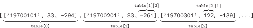
There are a few different ways to store two-dimensional data. To illustrate the most straightforward technique, let’s revisit the tabular data sets with which we worked in Chapter 8. One of the simplest was the CSV file containing monthly extreme temperature readings in Madison, Wisconsin from Exercise 8.4.6 (madison_temp.csv):
STATION,STATION_NAME,DATE,EMXT,EMNT
GHCND:USW00014837,MADISON DANE CO REGIONAL AIRPORT WI US,19700101,33,-294
GHCND:USW00014837,MADISON DANE CO REGIONAL AIRPORT WI US,19700201,83,-261
GHCND:USW00014837,MADISON DANE CO REGIONAL AIRPORT WI US,19700301,122,-139
 .
 .
 .
Because all of the data in this file is based on conditions at the same site, the first two columns are identical in every row. The third column contains the dates of the first of each month in which data was collected. The fourth and fifth columns contain the maximum and minimum monthly temperatures, respectively, which are in tenths of a degree Celsius (i.e., 33 represents 3.3° C). Previously, we would have extracted this data into three parallel lists containing dates, maximum temperatures, and minimum temperatures, like this:
def readData():
    """Read monthly extreme temperature data into a table.

    Parameters: none

    Return value: a list of lists containing monthly extreme
                  temperature data
    """

    dataFile = open('madison_temp.csv', 'r')
    header = dataFile.readline()
    dates = []
    maxTemps = []
    minTemps = []
    for line in dataFile:
        row = line.split(',')
        dates.append(row[2])
        maxTemps.append(int(row[3]))
        minTemps.append(int(row[4]))
    dataFile.close()
    return dates, maxTemps, minTemps
Alternatively, we may wish to extract tabular data into a single table. This is especially convenient if the data contains many columns. For example, the three columns above could be stored in a unified tabular structure like the following:
|
|
|
|---|---|---|
|
|
|
|
|
|
|
|
|
⋮ |
⋮ |
⋮ |
We can represent this structure as a list of rows, where each row is a list of values in that row. In other words, the table above can be stored like this:
[['19700101', 33, -294], ['19700201', 83, -261], ['19700301', 122, -139], ... ]
To better visualize this list as a table, we can reformat its presentation a bit:
[
  [ '19700101',  33, -294 ],
  [ '19700201',  83, -261 ],
  [ '19700301', 122, -139 ],
  ⋮
]
Notice that, in the function above, we already have each of these row lists contained in the list named row. Therefore, to create this structure, we can simply append each value of row, with the temperature values converted to integers and the first two redundant columns removed, to a growing list of rows named table:
def readData():
    """ (docstring omitted) """

    dataFile = open('madison_temp.csv', 'r')
    header = dataFile.readline()
    table = []
    for line in dataFile:
        row = line.split(',')
        row[3] = int(row[3])
        row[4] = int(row[4])
        table.append(row[2:]) # add a new row to the table
    dataFile.close()
    return table
Since each element of table is a list containing a row of this table, the first row is assigned to table[0], as illustrated below. Similarly, the second row is assigned to table[1] and the third row is assigned to table[2].
Reflection 9.1 How would you access the minimum temperature in February, 1970 (date value '19700201') from this list?
The minimum temperature in February, 1970 is the third value in the list table[1]. Since table[1] is a list, we can use indexing to access individual items contained in it. Therefore, the third value in table[1] is table[1][2], which equals -261 (i.e., -26.1° C), as indicated above. Likewise, table[2][1] is the maximum temperature in March, 1970: 122, or 12.2° C.
Reflection 9.2 In general, how can you access the value in row r and column c?
Notice that, for a particular value table[r][c], r is the index of the row and c is the index of the column. So if we know the row and column of any desired value, it is easy to retrieve that value with this convenient notation.
Now suppose we want to search this table for the minimum temperature in a particular month, given the corresponding date string. To access this value in the table, we will need both its row and column indices. We already know that the column index must be 2, since the minimum temperatures are in the third column. To find the correct row index, we need to search all of the values in the first column until we find the row that contains the desired string. Once we have the correct row index r, we can simply return the value of table[r][2]. The following function does exactly this.
def getMinTemp(table, date):
    """Return the minimum temperature for the month
       with the given date string.

    Parameters:
        table: a table containing extreme temperature data
        date: a date string

    Return value:
        the minimum temperature for the given date
        or None if the date does not exist
    """

    numRows = len(table)
    for r in range(numRows):
        if table[r][0] == date:
            return table[r][2]
    return None
The for loop iterates over the the indices of the rows in the table. For each row with index r, we check if the first value in that row, table[r][0], is equal to the date we are looking for. If it is, we return the value in column 2 of that row. On the other hand, if we get all the way through the loop without returning a value, the desired date must not exist, so we return None.
Exercises
From this point on, we will generally not specify what the name and parameters of a function should be. Instead, we would like you to design the function(s).
9.1.1. Show how the following table can be stored in a list named scores.
|
|
|
|
|
|
|
|
|
|
|
|
|
|
|
|
|
|
9.1.2. In the list you created above, how do you refer to each of the following?
(a) the SAT M value for student 10089
(b) the SAT CR value for student 11304
(c) the SAT M value for student 10305
(d) the SAT CR value for student 12007
9.1.3. Alternatively, a table could be stored as a list of columns.
(a) Show how to store the table in Exercise 9.1.1 in this way.
(b) Redo Exercise 9.1.2 using this new list.
(c) Why is this method less convenient when reading data in from a file?
9.1.4. Write a program that calls the readData function to read temperatures into a table, and then repeatedly asks for a date string to search for in the table. For each date string entered, your function should call the getMinTemp function to get the corresponding minimum temperature. For example, your function should print something like the following:
Minimum temperature for which date (q to quit)? 20050501
The minimum temperature for 20050501 was -2.2 degrees Celsius.

Minimum temperature for which date (q to quit)? 20050801
The minimum temperature for 20050801 was 8.3 degrees Celsius.

Minimum temperature for which date (q to quit)? q
9.1.5. Write a function that does the same thing as the getMinTemp function above, but returns the maximum temperature for a particular date instead.
9.1.6. If a data set contains a unique key value that is frequently searched, we can alternatively store the data in a dictionary. Each row in the table can be associated with its particular key value, which makes searching for a key value very efficient. For example, the temperature table
[
  [ '19700101',  33, -294 ],
  [ '19700201',  83, -261 ],
  [ '19700301', 122, -139 ]
]
could be stored in a dictionary as
{ '19700101': [33, -294],
  '19700201': [83, -261],
  '19700301': [122, -139] }
Rewrite the readData and getMinTemp functions so that the temperature data is stored in this way instead. Then incorporate these new functions into your program from Exercise 9.1.4.
9.1.7. Write a function that reads the earthquake data from the CSV file athttp://earthquake.usgs.gov/earthquakes/feed/v1.0/summary/2.5_month.csv into a table with four columns containing the latitude, longitude, depth, and magnitude of each earthquake. All four values should be stored as floating point numbers. (This is the same URL that we used in Section 8.4.)
9.1.8. Write a function that takes as a parameter a table returned by your function from Exercise 9.1.7 and prints a formatted table of the data. Your table should look similar to this:
Latitude    Longitude     Depth   Magnitude
--------    ---------     -----   ---------
   33.49      -116.46      19.8      1.1
   33.14      -115.65       2.1      1.8
   -2.52       146.12      10.0      4.6
   .
   .
   .
9.1.9. Write a function that takes as a parameter a table returned by your function from Exercise 9.1.7, and repeatedly prompts for a minimum earthquake magnitude. The function should then create a new table containing the rows corresponding to earthquakes with at least that magnitude, and then print this table using your function from Exercise 9.1.8. The output from your function should look similar to this:
     Minimum magnitude (q to quit)? 6.2

     Latitude    Longitude     Depth   Magnitude
     --------    ---------     -----   ---------
       -46.36        33.77      10.0      6.2
       -37.68       179.69      22.0      6.7
         1.93       126.55      35.0      7.1
        -6.04       148.21      43.2      6.6

     Minimum magnitude (q to quit)? 7

     Latitude    Longitude     Depth   Magnitude
     --------    ---------     -----   ---------
         1.93       126.55      35.0      7.1

     Minimum magnitude (q to quit)? 8
     There were no earthquakes with magnitude at least 8.0.

     Minimum magnitude (q to quit)? q
9.2 THE GAME OF LIFE
A cellular automaton is a rectangular grid of discrete cells, each of which has an associated state or value. Each cell represents an individual entity, such as an organism or a particle. At each time step, every cell can simultaneously change its state according to some rule that depends only on the states of its neighbors. Depending upon on the rules used, cellular automata may evolve global, emergent behaviors based only on these local interactions.
The most famous example of a cellular automaton is the Game of Life, invented by mathematician John Conway in 1970. In the Game of Life, each cell can be in one of two states: alive or dead. At each time step, the makeup of a cell’s neighborhood dictates whether or not it will pass into the next generation alive (or be reborn if it is dead). Depending upon the initial configuration of cells (which cells are initially alive and which are dead), the Game of Life can produce amazing patterns.
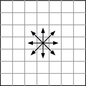
We consider each cell in the Game of Life to have eight neighbors, as illustrated below:
In each step, each of the cells simultaneously observes the states of its neighbors, and may change its state according to the following rules:
If a cell is alive and has fewer than two live neighbors, it dies from loneliness.
If a cell is alive and has two or three live neighbors, it remains alive.
If a cell is alive and has more than three live neighbors, it dies from overcrowding.
If a cell is dead and has exactly three live neighbors, it is reborn.
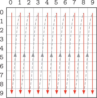
To see how these rules affect the cells in the Game of Life, consider the initial configuration in the top left of Figure 9.1. Dead cells are represented by white squares and live cells are represented by black squares. To apply rule 1 to the initial configuration, we need to check whether there are any live cells with fewer than two live neighbors. As illustrated below, there are two such cells, each marked with D.

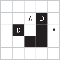
According to rule 1, these two cells will die in the next generation. To apply rule 2, we need to check whether there are any live cells that have two or three live neighbors. Since this rule applies to the other three live cells, they will remain alive into the next generation. There are no cells that satisfy rule 3, so we move on to rule 4. There are two dead cells with exactly three live neighbors, marked with A. According to rule 4, these two cells will come alive in the next generation.
Reflection 9.3 Show what the second generation looks like, after applying these rules.
The figure in the top center of Figure 9.1 shows the resulting second generation, followed by generations three, four, and five. After five generations, as illustrated in the bottom center of Figure 9.1, the grid has returned to its initial state, but it has moved one cell down and to the right of its initial position. If we continued computing generations, we would find that it would continue in this way indefinitely, or until it collides with a border. For this reason, this initial configuration generates what is known as a “glider.”

Creating a grid
To implement this cellular automaton, we first need to create an empty grid of cells. For simplicity, we will keep it relatively small, with 10 rows and 10 columns. We can represent each cell by a single integer value which equals 1 if the cell is alive or 0 if it is dead. For clarity, it is best to assign these values to meaningful names:
ALIVE = 1
DEAD = 0
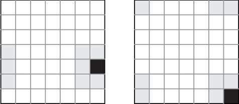
An initially empty grid, like the one on the left side of Figure 9.2, will be represented by a list of row lists, each of which contains a zero for every column. For example, the list on the right side of Figure 9.2 represents the grid to its left.
Reflection 9.4 How can we easily create a list of many zeros?
If the number of columns in the grid is assigned to columns, then each of these rows can be created with a for loop:
row = []
for c in range(columns):
    row.append(DEAD)
We can then create the entire grid by simply appending a copy of row for every row in the grid to a list named grid:
def makeGrid(rows, columns):
    """Create a rows x columns grid of zeros.

    Parameters:
        rows: the number of rows in the grid
        columns: the number of columns in the grid

    Return value: a list of ROWS lists of COLUMNS zeros
    """

    grid = []

    for r in range(rows):
        row = []
        for c in range(columns):
            row.append(DEAD)
        grid.append(row)
    return grid
This nested loop can actually be simplified somewhat by substituting
row = [DEAD] * columns
for the three statements that construct row because all of the values in each row are the same.
Initial configurations
The cellular automaton will evolve differently, depending upon the initial configuration of alive and dead cells. (There are several examples of this in the exercises at the end of this section.) We will assume that all cells are dead initially, except for those we explicitly specify. Each cell can be conveniently represented by a (row, column) tuple. The coordinates of the initially live cells can be stored in a list of tuples, and passed into the following function to initialize the grid. (Recall that a tuple is like a list, except that it is immutable and enclosed in parentheses instead of square brackets.)
def initialize(grid, coordinates):
    """Set a given list of coordinates to 1 in the grid.

    Parameters:
        grid: a grid of values for a cellular automaton
        coordinates: a list of coordinates

    Return value: None
    """

    for (r, c) in coordinates:
        grid[r][c] = ALIVE
The function iterates over the list of tuples and sets the cell at each position to be alive. For example, to match the initial configuration in the upper left of Figure 9.1, we would pass in the list
[(1, 3), (2, 3), (3, 3), (3, 2), (2, 1)]
Notice that by using a generic tuple as the index variable, we can conveniently assign the two values in each tuple in the list to r and c.
Box 9.1: NumPy arrays in two dimensions
Two-dimensional (and higher) data can also be represented with a NumPy array object. (See Box 8.1.) As in one dimension, we can initialize an array by either passing in a list, or passing a size to one of several functions that fill the array with particular values. Here are some examples.
>>> import numpy
>>> temps = numpy.array([[3.3, -29.4], [8.3, -26.1], [12.2, -13.9]])
>>> temps
array([[  3.3, -29.4],
       [  8.3, -26.1],
       [ 12.2, -13.9]])
>>> grid = numpy.zeros((2, 4)) # zero-filled with 2 rows, 4 cols
>>> grid
array([[ 0., 0., 0., 0.],
       [ 0., 0., 0., 0.]])
In the second case, the tuple (2, 4) specifies the “shape” of the array: three rows and four columns. We can modify individual array elements with indexing by simply specifying the comma-separated row and column in a single pair of square braces:
>>> grid[1, 3] = 1
>>> grid
array([[ 0., 0., 0.,  0.],
       [ 0., 0., 0.,  1.]])
As we saw in Box 8.1, the real power of NumPy arrays lies in the ability to change every element in a single statement. For example, the following statement adds one to every element of the temps array.
>>> temps = temps + 1
>>> temps
array([[  4.3, -28.4],
       [  9.3, -25.1],
       [ 13.2, -12.9]])
For more details, see http://numpy.org.
Surveying the neighborhood
To algorithmically carry out the rules in the Game of Life, we will need a function that returns the number of live neighbors of any particular cell.
Reflection 9.5 Consider a cell at position (r, c). What are the coordinates of the eight neighbors of this cell?
The coordinates of the eight neighbors are visualized in the following grid with coordinates (r, c) in the center.
(r – 1, c – 1) |
(r – 1, c) |
(r – 1, c + 1) |
(r, c – 1) |
(r, c) |
(r, c + 1) |
(r + 1, c – 1) |
(r + 1, c) |
(r + 1, c + 1) |
We could use an eight-part if/elif/else statement to check whether each neighbor is alive. However, an easier approach is illustrated below.
def neighborhood(grid, row, column):
    """Finds the number of live neighbors of the cell in the
       given row and column.

    Parameters:
        grid: a two-dimensional grid of cells
        row: the row index of a cell
        column: the column index of a cell

    Return value:
        the number of live neighbors of the cell at (row, column)
    """

    offsets = [ (-1, -1), (-1, 0), (-1, 1),
                (0, -1),           (0, 1),
                (1, -1),  (1, 0),  (1, 1)   ]
    rows = len(grid)
    columns = len(grid[0])
    count = 0
    for offset in offsets:
        r = row + offset[0]
        c = column + offset[1]
        if (r >= 0 and r < rows) and (c >= 0 and c < columns):
            if grid[r][c] == ALIVE:
                count = count + 1
    return count
The list offsets contains tuples with the offsets of all eight neighbors. We iterate over these offsets, adding each one to the given row and column to get the coordinates of each neighbor. Then, if the neighbor is on the grid and is alive, we increment a counter.
Performing one pass
Once we can count the number of live neighbors, we can simulate one generation by iterating over all of the cells and updating them appropriately. But before we look at how to iterate over every cell in the grid, let’s consider how we can iterate over just the first row.
Reflection 9.6 What is the name of the first row of grid?
The first row of grid is named grid[0]. Since grid[0] is a list, we already know how to iterate over it, either by value or by index.
Reflection 9.7 Should we iterate over the indices of grid[0] or over its values? Does it matter?
As we saw above, we need to access a cell’s neighbors by specifying their relative row and column indices. So we are going to need to know the indices of the row and column of each cell as we iterate over them. This means that we need to iterate over the indices of grid[0], which are also its column indices, rather than over its values. Therefore, the for loop looks like this, assuming the number of columns is assigned to the variable name columns:
for c in range(columns):
    # update grid[0][c] here
Notice that, in this loop, the row number stays the same while the column number (c) increases. We can generalize this idea to iterate over any row with index r by simply replacing the row index with r:
for c in range(columns):
    # update grid[r][c] here
Now, to iterate over the entire grid, we need to repeat the loop above with values of r ranging from 0 to rows-1, where rows is assigned the number of rows in the grid. We can do this by nesting the loop above in the body of another for loop that iterates over the rows:
for r in range(rows):
    for c in range(columns):
        # update grid[r][c] here
Reflection 9.8 In what order will the cells of the grid be visited in this nested loop? In other words, what sequence of r,c values does the nested loop generate?
The value of r is initially set to 0. While r is 0, the inner for loop iterates over values of c from 0 to COLUMNS - 1. So the first cells that will be visited are
grid[0][0], grid[0][1], grid[0][2], ..., grid[0][9]
Once the inner for loop finishes, we go back up to the top of the outer for loop. The value of r is incremented to 1, and the inner for loop executes again. So the next cells that will be visited are
grid[1][0], grid[1][1], grid[1][2], ..., grid[1][9]
This process repeats with r incremented to 2, 3, ..., 9, until finally the cells in the last row are visited:
grid[9][0], grid[9][1], grid[9][2], ..., grid[9][9]
Therefore, visually, the cells in the grid are being visited row by row:
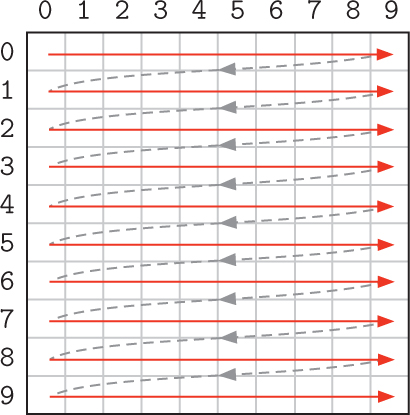
Reflection 9.9 How would we change the nested loop so that the cells in the grid are visited column by column instead?
To visit the cells column by column, we can simply swap the positions of the loops:
for c in range(columns):
    for r in range(rows):
        # update grid[r][c] here
Reflection 9.10 In what order are the cells of the grid visited in this new nested loop?
In this new nested loop, for each value of c, the inner for loop iterates all of the values of r, visiting all of the cells in that column. So the first cells that will be visited are
grid[0][0], grid[1][0], grid[2][0], ..., grid[9][0]
Then the value of c is incremented to 1 in the outer for loop, and the inner for loop executes again. So the next cells that will be visited are
grid[0][1], grid[1][1], grid[2][1], ..., grid[9][1]
This process repeats with consecutive values of c, until finally the cells in the last column are visited:
grid[0][9], grid[1][9], grid[2][9], ..., grid[9][9]
Therefore, in this case, the cells in the grid are being visited column by column instead:
Reflection 9.11 Do you think the order in which the cells are updated in a cellular automaton matters?
In most cases, the order does not matter. We will update the cells row by row.
Updating the grid
Now we are ready to implement one generation of the Game of Life by iterating over all of the cells and applying the rules to each one. For each cell in position (r, c), we first need to find the number of neighbors by calling the neighbors function that we wrote above. Then we set the cell’s new value, if it changes, according to the four rules, as follows.
for r in range(rows):
    for c in range(columns):
        neighbors = neighborhood(grid, r, c)
        if grid[r][c] == ALIVE and neighbors < 2:               # rule 1
            grid[r][c] = DEAD
        elif grid[r][c] == ALIVE and neighbors > 3:             # rule 3
            grid[r][c] = DEAD
        elif grid[r][c] == DEAD and neighbors == 3:             # rule 4
            grid[r][c] = ALIVE
Reflection 9.12 Why is rule 2 not represented in the code above?
Since rule 2 does not change the state of any cells, there is no reason to check for it.
Reflection 9.13 There is one problem with the algorithm we have developed to update cells. What is it? (Think about the values referenced by the neighborhood function when it is applied to neighboring cells. Are the values from the previous generation or the current one?)
To see the subtle problem, suppose that we change cell (r, c) from alive to dead. Then, when the live neighbors of the next cell in position (r, + 1, c) will not be counted. But it should have been because it was alive in the previous generation. To fix this problem, we cannot modify the grid directly while we are updating it. Instead, we need to make a copy of the grid before each generation. When we count live neighbors, we will look at the original grid, but make modifications in the copy. Then, after we have looked at all of the cells, we can update the grid by assigning the updated copy to the main grid. These changes are shown below in red.
newGrid = copy.deepcopy(grid)
for r in range(rows):
    for c in range(columns):
        neighbors = neighborhood(grid, r, c)
        if grid[r][c] == ALIVE and neighbors < 2:            # rule 1
            newGrid[r][c] = DEAD
        elif grid[r][c] == ALIVE and neighbors > 3:          # rule 3
            newGrid[r][c] = DEAD
        elif grid[r][c] == DEAD and neighbors == 3:          # rule 4
            newGrid[r][c] = ALIVE
grid = newGrid
The deepcopy function from the copy module creates a completely independent copy of the grid.
Now that we can simulate one generation, we simply have to repeat this process to simulate many generations. The complete function is shown below. The grid is initialized with our makeGrid and initialize functions, then the nested loop that updates the grid is further nested in a loop that iterates for a specified number of generations.
def life(rows, columns, generations, initialCells):
    """Simulates the Game of Life for the given number of
       generations, starting with the given live cells.

    Parameters:
        rows: the number of rows in the grid
        columns: the number of columns in the grid
        generations: the number of generations to simulate
        initialCells: a list of (row, column) tuples indicating
                      the positions of the initially alive cells

    Return value:
        the final configuration of cells in a grid
    """

    grid = makeGrid(rows, columns)
    initialize(grid, initialCells)
    for g in range(generations):

        newGrid = copy.deepcopy(grid)
        for r in range(rows):
            for c in range(columns):
                neighbors = neighborhood(grid, r, c)
                if grid[r][c] == ALIVE and neighbors < 2:                 # rule 1
                    newGrid[r][c] = DEAD
                elif grid[r][c] == ALIVE and neighbors > 3:               # rule 3
                    newGrid[r][c] = DEAD
                elif grid[r][c] == DEAD and neighbors == 3:               # rule 4
                    newGrid[r][c] = ALIVE
        grid = newGrid
    return grid
On the book web site, you can find an enhanced version of this function that uses turtle graphics to display the evolution of the system with a variety of initial configurations.
Exercises
9.2.1. Download the enhanced Game of Life program from the book web site and run it with each of the following lists of coordinates set to be alive in the initial configuration. Use at least a 50
(a) [(1, 3), (2, 3), (3, 3), (3, 2), (2, 1)]
(b) [(9, 10), (10, 10), (11, 10)]
(c) [(10, c + 1), (10, c + 4), (11, c), (12, c),
    (12, c + 4), (13, c), (13, c + 1), (13, c + 2),
    (13, c + 3)] with c = COLUMNS - 5
(d) [(r + 1, c + 2), (r + 2, c + 4), (r + 3, c + 1),
    (r + 3, c + 2), (r + 3, c + 5), (r + 3, c + 6),
    (r + 3, c + 7)] with r = ROWS // 2 and c = COLUMNS // 2
9.2.2. Modify the neighborhood function so that it treats the grid as if all four sides “wrap around.” For example, in the 7 × 7 grid below on the left, the neighbors of (4, 6) include (3, 0), (4, 0), and (5, 0). In the grid on the right, the neighbors of the corner cell (6, 6) include (0, 0), (0, 5), (0, 6), (5, 0), and (6, 0).
9.2.3. Write a function that prints the contents of a parameter named grid, which is a list of lists. The contents of each row should be printed on one line with spaces in between. Each row should be printed on a separate line.
9.2.4. Write a function that takes an integer n as a parameter, and returns an n × n multiplication table as a list of lists. The value in row r and column c should be the product of r and c.
9.2.5. Write a function that takes an integer n as a parameter, and returns an n × n grid (list of lists) in which all cells on the main diagonal contain a 1 and the rest of the cells contain a 0. For example, if n = 5, your function should return the grid
[[1, 0, 0, 0, 0],
 [0, 1, 0, 0, 0],
 [0, 0, 1, 0, 0],
 [0, 0, 0, 1, 0],
 [0, 0, 0, 0, 1]]
9.2.6. Write a function that takes an integer n as a parameter, and returns an n × n grid (list of lists) in which all cells on and below the main diagonal contain a 1 and the rest of the cells contain a 0. For example, if n = 5, your function should return
[[1, 0, 0, 0, 0],
 [1, 1, 0, 0, 0],
 [1, 1, 1, 0, 0],
 [1, 1, 1, 1, 0],
 [1, 1, 1, 1, 1]]
9.2.7. Write a function that takes as a parameter a two-dimensional grid (list of lists) of numbers, and prints (a) the sum of each row, (b) the sum of each column, and (c) the sum of all the entries.
9.2.8. Write a function that takes as parameters a two-dimensional grid (list of lists) and a value to search for, and returns the (row, column) where the value first appears, if it appears anywhere in the grid, and (−1, −1) otherwise.
9.2.9. Write a function that returns a two-dimensional grid (list of lists) representation of an 8 × 8 checkerboard in which the squares in both directions alternate between the values 'B' and 'W'.
9.2.10. A magic square is a grid of numbers for which the sum of all the columns and all the rows is the same. For example, in the magic square below, all the rows and columns add up to 15.
5 |
7 |
3 |
1 |
6 |
8 |
9 |
2 |
4 |
The following algorithm generates magic squares with odd-length sides, using the consecutive numbers 1, 2, 3, ....
(a) Randomly put 1 in some position in your square.
(b) Look in the square diagonally to the lower right of the previous square, wrapping around to the if you go off the edge to the right or bottom.
If this square is unoccupied, put the next number there.
Otherwise, put the next number directly above the previous number (again wrapping to the bottom if you are on the top row).
(c) Continue step (b) until all the positions are filled.
Write a function that takes an odd integer n as a parameter and returns an n × n magic square.
9.2.11. A two-dimensional grid can also be stored as a dictionary in which the keys are tuples representing grid positions. For example, the small grid
[ [0, 1],
  [1, 1] ]
would be stored as the following dictionary:
{ (0, 0): 0,
  (0, 1): 1,
  (1, 0): 1,
  (1, 1): 1 }
Rewrite the Game of Life program on the book web site so that it stores the grid in this way instead. The following four functions will need to change: emptyGrid, initialize, neighborhood, and life.
9.3 DIGITAL IMAGES
Digital photographs and other images are also “flat” two-dimensional objects that can be manipulated with the same techniques that we discussed in previous sections.
Colors
A digital image is a two-dimensional grid (sometimes called a bitmap) in which each cell, called a pixel (short for “picture element”), contains a value representing its color. In a grayscale image, the colors are limited to shades of gray. These shades are more commonly referred to as levels of brightness or luminance, and in theory are represented by values between 0 and 1, 0 being black and 1 being white. As we briefly explained in Box 3.2, each pixel in a color image can be represented by a (red, green, blue), or RGB, tuple. Each component, or channel, of the tuple represents the brightness of the respective color. The value (0, 0, 0) is black and (1, 1, 1) is white. Values between these can represent any color in the spectrum. For example, (0, 0.5, 0) is a medium green and (1, 0.5, 0) is orange. In practice, each channel is represented by eight bits (one byte) or, equivalently, a value between 0 and 255. So black is represented by (0, 0, 0) or
00000000 00000000 00000000 ,
white is (255, 255, 255) or
11111111 11111111 11111111 ,
and orange is (255, 127, 0) or
11111111 01111111 00000000.
Box 9.2: Additive vs. subtractive color models
Colors in digital images are usually represented in one of two ways. In the text, we focus on the RGB color model because it is the most common, especially for digital cameras and displays. RGB is called an additive color model because the default “no color” (0, 0, 0) is black, and adding all of the colors, represented by (255, 255, 255), is white. In contrast, printers use a subtractive color model that “subtracts” from the brightness of a white paper background by applying color. The most common subtractive color model is CMY (short for “Cyan Magenta Yellow”). In CMY, the “no color” (0, 0, 0) is white, and (255, 255, 255) combines cyan, magenta, and yellow at full intensities to produce black. In practice, a black channel is added to the CMY color model because black is so common in print, and combining cyan, magenta, and yellow to produce black tends to be both imperfect and expensive in practice. The resulting four-color model is called CMYK where K stands for “Key” or “blacK,” depending on who you ask.
Some color models also allow an alpha channel to specify transparency. An alpha value of 0 means the color is completely transparent (i.e., invisible), 255 means it is opaque, and values in between correspond to degrees of translucency. Translucency effects are implemented by combining the translucent color in the foreground with the background color to an extent specified by the alpha channel. In other words,
displayed color = α. foreground color + (1 - α). background color.
RGB is most commonly used for images produced by digital cameras and viewed on a screen. Another encoding, called CMYK is used for print. See Box 9.2 for more details.
Reflection 9.14 If we use eight bits to represent the intensity of each channel, can we still represent any color in the spectrum? If not, how many different colors can we represent?
Using eight bits per channel, we cannot represent the continuous range of values between 0 and 1 that would be necessary to represent any color in the spectrum. In effect, we are only able to represent 254 values between 0 and 1: 1/255, 2/255, ..., 254/255. This is another example of how some objects represented in a computer are limited versions of those existing in nature. Looking at it another way, by using 8 bits per channel, or 24 bits total, we can represent 224 = 16, 777, 216 distinct colors. The good news is that, while this does not include all the colors in the spectrum, it is greater than the number of colors distinguishable by the human eye.
Reflection 9.15 Assuming eight bits are used for each channel, what RGB tuple represents pure blue? What tuple represents purple? What color is (0, 128, 128)?
Bright blue is (0, 0, 255) and any tuple with equal parts red and blue, for example (128, 0, 128) is a shade of purple. The tuple (0, 128, 128), equal parts medium green and medium blue, is teal.
Box 9.3: Image storage and compression
Digital images are stored in a variety of file formats. Three of the most common are BMP, GIF, and JPEG. The technical details of each format can be quite complex, so we will just highlight the key differences, advantages, and disadvantages.
All image files begin with a short header that contains information about the dimensions of the image, the number of bits that are used to encode the color of each pixel (usually 24), and other format-specific characteristics. The header is followed by information about the actual pixels. In a BMP (short for “BitMaP”) file, the pixels are simply stored row by row, starting from the bottom left corner (upside down). Assuming 24-bit color, the size of a BMP file is roughly three bytes per pixel. For example, the 300 × 200 pixel color image in Figure 9.3 requires about 300 · 200 · 3 = 180,000 bytes ≈ 180 KB in BMP format.
GIF (short for “Graphics Interchange Format”) files try to cut down on the amount of memory required to store an image in two ways. First, rather than store the actual color of each pixel individually, GIF files encode each pixel with an 8-bit index into a table of 28 = 256 image-dependent colors. Second, GIF files compress the resulting pixel data using the Lempel-Ziv-Welch (LZW) data compression algorithm (see Box 6.1). This compression algorithm is lossless, meaning that the original data can be completely recovered from the compressed data, resulting in no loss of image quality. So the size of a GIF file is typically less than one byte per pixel. The color image in Figure 9.3 requires about 46 KB in GIF format.
JPEG (short for “Joint Photographic Experts Group,” the name of the group that created it) files use a lossy compression algorithm to further cut down on their size. “Lossy” means that information is lost from the original image. However, the lossy compression algorithm used in JPEG files selectively removes characteristics that are less noticeable to the naked eye, resulting in very little noticeable difference in quality. The color image in Figure 9.3 requires about 36 KB in JPEG format.
The digital images produced by digital cameras can be quite large. For example, a high quality camera can produce an image that is about 5120 pixels wide and 3413 pixels high, and therefore contains a total of 5120 × 3413 = 17, 474, 560 pixels. At one byte per pixel, a grayscale image of this size would require about 17 MB of storage. A 5120 by 3413 color image requires 5120 × 3413 × 3 = 52, 423, 680 bytes, or about 50 MB, of storage, since it requires 24 bits, or three bytes, per pixel. In practice, color image files are compressed to take up much less space. (See Box 9.3.)
Image filters
To illustrate some basic image processing techniques, let’s consider how we can produce a grayscale version of a color image. An operation such as this is known as an image filter algorithm. Photo-editing software typically includes several different image filters for enhancing digital photographs.
To change an image to grayscale, we need to convert every color pixel (an RGB tuple) to a gray pixel with similar brightness. A white pixel (RGB color (255, 255, 255)) is the brightest, so we would map this to a grayscale brightness of 255 while a black pixel (RGB color (0, 0, 0)) is the least bright, so we would map this to a grayscale brightness of 0.
Reflection 9.16 How can we compute the brightness of a color pixel in general?
Consider the RGB color (250, 50, 200). The red and blue channels of this color contribute a lot of brightness to the color while the green channel does not. So, to estimate the overall brightness, we can simply average the three values. In this case, (250 + 50 + 200)/3 ≈ 167. In RGB, any tuple with equal parts red, green, and blue will be a shade of gray. Therefore, we can encode this shade of gray in RGB with the tuple (167, 167, 167). A function to perform this conversion is straightforward:
def color2gray(color):
    """Convert a color to a shade of gray.

    Parameter:
        color: a tuple representing an RGB color

    Return value: a tuple representing an equivalent gray
    """

    brightness = (color[0] + color[1] + color[2]) // 3
    return (brightness, brightness, brightness)
The parameter color is a three-element tuple of integers between 0 and 255. The function computes the average of the three channels and returns a tuple representing a shade of gray with that brightness.
To apply this transformation to an entire image, we need to iterate over the positions of all of the pixels. Since an image is a two-dimensional object, we can process its pixels row by row as we did in the previous section:
for r in range(rows):
    for c in range(columns):
        # process the pixel at position (r, c)
To be consistent with the language typically used in image processing, we will use different names for the variables, however. Rather than referring to the size of an image in terms of rows and columns, we will use height and width. And we will use x and y (with (0, 0) in the top left corner) to denote the horizontal and vertical positions of a pixel instead of the row and column numbers. So the following is equivalent to the nested loop above:
for y in range(height):
    for x in range(width):
        # process the pixel at coordinates (x, y)
The standard Python module for displaying images (and creating graphical interface elements like windows and buttons) is called tkinter (This name is short for “Tk interface.” Tk is a widely used graphical programming package that predates Python; tkinter provides an “interface” to Tk.) Because simple image manipulation in tkinter is slightly more complicated than we would like, we will interact with tkinter indirectly through a simple class named Image. The Image class is available in the module image.py on the book web site. Download this file and copy it into the same folder as your programs for this section.
The following program illustrates how to use the Image class to read a digital image file, iterate over its pixels, and produce a new image that is a grayscale version of the original. Each of the methods and functions below is described in Appendix B.8.
import image

def grayscale(photo):
    """Convert a color image to grayscale.

    Parameter:
        photo: an Image object

    Return value: a new grayscale Image object
    """

    width = photo.width()
    height = photo.height()
    newPhoto = image.Image(width, height, title = 'Grayscale image')
    for y in range(height):
        for x in range(width):
            color = photo.get(x, y)
            newPhoto.set(x, y, color2gray(color))
    return newPhoto

def main():
    penguin = image.Image(file = 'penguin.gif', title = 'Penguin')
    penguinGray = grayscale(penguin)
    penguin.show()
    penguinGray.show()
    image.mainloop()

main()
Let’s look at the grayscale function first. The lone parameter named photo is the Image object that we want to turn to grayscale. The first two statements in the function call the width and height methods of photo to get the image’s dimensions. Then the third statement creates a new, empty Image object with the same dimensions. This will be our grayscale image. Next, we iterate over all of the pixels in photo. Inside the nested loop, we call the get method to get the color of the pixel at each position (x,y) in photo. The color is returned as a three-element tuple of integers between 0 and 255. Next, we set the pixel at the same position in newPhoto to the color returned by the color2gray function that we wrote above. Once the nested loop has finished, we return the grayscale photo.
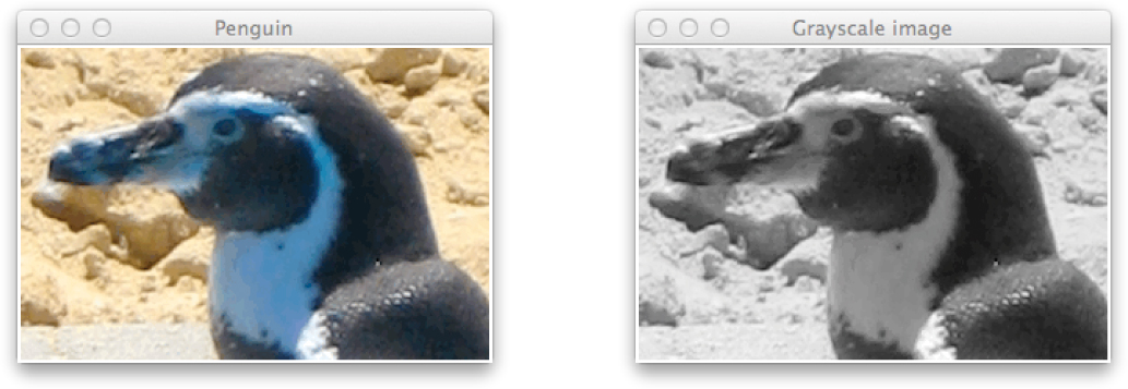
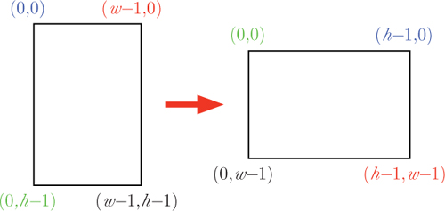
Figure 9.4 Rotating an image 90 degrees clockwise. After rotation, the corners with the same colors should line up. The width and height of the image are represented by w and h, respectively.
In the main function, we create an Image object named penguin from a GIF file named penguin.gif that can be found on the book web site. (GIF is a common image file format; see Box 9.3 for more about image files.) We then call the grayscale function with penguin, and assign the resulting grayscale image to penguinGray. Finally, we display both images in their own windows by calling the show method of each one. The mainloop function at the end causes the program to wait until all of the windows have been closed before it quits the program. The results are shown in Figure 9.3. This simple filter is just the beginning; we leave several other fun image filters as exercises.
Transforming images
There are, of course, many other ways we might want to transform an image. For example, we commonly need to rotate landscape images 90 degrees clockwise. This is illustrated in Figure 9.4. From the figure, we notice that the pixel in the corner at (0, 0) in the original image needs to be in position (h – 1, 0) after rotation. Similarly, the pixel in the corner at (w – 1, 0) needs to be in position (h–1, w –1) after rotation. The transformations for all four corners are shown below.
Before |
After |
|
|---|---|---|
(0, 0) |
⇒ |
(h – 1, 0) |
(w – 1, 0) |
⇒ |
(h – 1, w - 1) |
(w – 1, h – 1) |
⇒ |
(0, w – 1) |
(0, h – 1) |
⇒ |
(0, 0) |
Reflection 9.17 Do you see a pattern in these transformations? Use this pattern to infer a general rule about where each pixel at coordinates (x, y) should be in the rotated image.
The first thing to notice is that the width and height of the image are swapped, so the x and y coordinates in the original image need to be swapped in the rotated image. However, just swapping the coordinates leads to the mirror image of what we want. Notice from the table above that the y coordinate of each rotated corner is the same as the x coordinate of the corresponding original corner. But the x coordinate of each rotated corner is the h – 1 minus the y coordinate of the corresponding corner in the original image. So we want to draw each pixel at (x, y) in the original (h – 1 – y, x) in the rotated image. The following function does this. Notice that it is identical to the grayscale function, with the exceptions of parts of two statements in red.
def rotate90(photo):
    """Rotate an image 90 degrees clockwise.

     Parameter:
         photo: an Image object

     Return value: a new rotated Image object
     """

     width = photo.width()
     height = photo.height()
     newPhoto = image.Image(height, width, title = 'Rotated image')
     for y in range(height):
         for x in range(width):
             color = photo.get(x, y)
             newPhoto.set(height - y - 1, x, color)
     return newPhoto
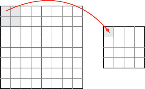
Let’s look at one more example, and then we will leave several more as exercises. Suppose we want to reduce the size of an image to one quarter of its original size. In other words, we want to reduce both the width and height by half. In the process, we are obviously going to lose three quarters of the pixels. Which ones do we throw away? One option would be to group the pixels of the original image into 2 × 2 blocks and choose the color of one of these four pixels for the corresponding pixel in the reduced image, as illustrated in Figure 9.5. This is accomplished by the following function. Again, it is very similar to the previous functions.
def reduce(photo):
    """Reduce an image to one quarter of its size.

    Parameter:
        photo: an Image object

    Return value: a new reduced Image object
    """

    width = photo.width()
    height = photo.height()
    newPhoto = image.Image(width // 2, height // 2,
                           title = 'Reduced image')
    for y in range(0, height, 2):
        for x in range(0, width, 2):
            color = photo.get(x, y)
            newPhoto.set(x // 2, y // 2, color)
    return newPhoto
Although this works, a better option would be to average the three channels of the four pixels in the block, and use this average color in the reduced image. This is left as an exercise.
Once we have filters like this, we can combine them in any way we like. For example, we can create an image of a small, upside down, grayscale penguin:
def main():
    penguin = image.Image(file = 'penguin.gif', title = 'Penguin')
    penguinSmall = reduce(penguin)
    penguinGray = grayscale(penguinSmall)
    penguinRotate1 = rotate90(penguinGray)
    penguinRotate2 = rotate90(penguinRotate1)
    penguinRotate2.show()
    image.mainloop()
By implementing some of the additional filters in the exercises below, you can devise many more fun creations.
Exercises
9.3.1. Real grayscale filters take into account how different colors are perceived by the human eye. Human sight is most sensitive to green and least sensitive to blue. Therefore, for a grayscale filter to look more realistic, the intensity of the green channel should contribute the most to the grayscale luminance and the intensity of the blue channel should contribute the least. The following formula is a common way to weigh these intensities:
luminance = 0.2126 ˙ red + 0.7152 ˙ green + 0.0722 ˙ blue
Modify the color2gray function in the text so that it uses this formula instead.
9.3.2. The colors in an image can be made “warmer” by increasing the yellow tone. In the RGB color model, this is accomplished by increasing the intensities of both the red and green channels. Write a function that returns an Image object that is warmer than the original by some factor that is passed as a parameter. If the factor is positive, the image should be made warmer; if the factor is negative, it should be made less warm.
9.3.3. The colors in an image can be made “cooler” by increasing the intensity of the blue channel. Write a function that returns an Image object that is cooler than the original by some factor that is passed as a parameter. If the factor is positive, the image should be made cooler; if the factor is negative, it should be made less cool.
9.3.4. The overall brightness in an image can be adjusted by increasing the intensity of all three channels. Write a function that returns an Image object that is brighter than the original by some factor that is passed as a parameter. If the factor is positive, the image should be made brighter; if the factor is negative, it should be made less bright.
9.3.5. A negative image is one in which the colors are the opposite of the original. In other words, the intensity of each channel is 255 minus the original intensity. Write a function that returns an Image object that is the negative of the original.
9.3.6. Write a function that returns an Image object that is a horizontally flipped version of the original. Put another way, the image should be reflected along an imaginary vertical line drawn down the center. See the example on the left of Figure 9.6.
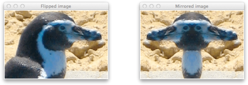
Figure 9.6 Horizontally flipped and mirrored versions of the original penguin image from Figure 9.3.
9.3.7. Write a function that returns an Image object with left half the same as the original but with right half that is a mirror image of the original. (Imagine placing a mirror along a vertical line down the center of an image, facing the left side.) See the example on the right of Figure 9.6.
9.3.8. In the text, we wrote a function that reduced the size of an image to one quarter of its original size by replacing each 2 × 2 block of pixels with the pixel in the top left corner of the block. Now write a function that reduces an image by the same amount by instead replacing each 2 × 2 block with a pixel that has the average color of the pixels in the block.
9.3.9. An image can be blurred by replacing each pixel with the average color of its eight neighbors. Write a function that returns a blurred version of the original.
9.3.10. An item can be further blurred by repeatedly applying the blur filter you wrote above. Write a function that returns a version of the original that has been blurred any number of times.
9.3.11. Write a function that returns an image that is a cropped version of the original. The portion of the original image to return will be specified by a rectangle, as illustrated below.
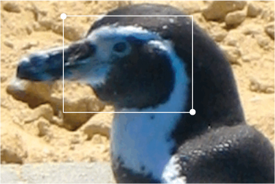
The function should take in four additional parameters that specify the (x, y) coordinates of the top left and bottom right corners (shown above) of the crop rectangle.
9.4 SUMMARY
As we saw in the previous chapter, a lot of data is naturally stored in two-dimensional tables. So it makes sense that we would also want to store this data in a two-dimensional structure in a program. We discussed two ways to do this. First, we can store the data in a list of lists in which each inner list contains one row of data. Second, in Exercises 9.1.6 and 9.2.11, we looked at how two-dimensional data can be stored in a dictionary. The latter representation has the advantage that it can be searched efficiently, if the data has an appropriate key value.
Aside from storing data, two-dimensional structures have many other applications. Two-dimensional cellular automata are widely used to model a great variety of phenomena. The Game of Life is probably the most famous, but cellular automata can also be used to model actual cellular systems, pigmentation patterns on sea shells, climate change, racial segregation (Project 9.1), ferromagnetism (Project 9.2), and to generate pseudorandom numbers. Digital images are also stored as two-dimensional structures, and image filters are simply algorithms that manipulate these structures.
9.5 FURTHER DISCOVERY
The chapter epigraph is from Flatland: A Romance of Many Dimensions, written by Edwin A. Abbott in 1884 [1].
If you are interested in learning more about cellular automata, or emergent systems in general, we recommend Turtles, Termites, and Traffic Jams by Mitchell Resnick [44] and Emergence by Steven Johnson [22] as good places to start. Also, we recommend Agent-Based Models by Nigel Gilbert [15] if you would like to learn more about using cellular automata in the social sciences. Biological Computation by Ehud Lamm and Ron Unger [27] is about using biologically-inspired computational techniques, such as cellular automata, genetic algorithms and artificial neural networks, to solve hard problems.
9.6 PROJECTS
Project 9.1 Modeling segregation
In 1971, Thomas Schelling (who in 2005 was co-recipient of the Nobel Prize in Economics) proposed a theoretical model for how racial segregation occurs in urban areas [47]. In the Schelling model, as it is now called, individuals belonging to one of two groups live in houses arranged in a grid. Let’s call the two groups the Plain-Belly Sneetches and the Star-Belly Sneetches [50]. Each cell in the grid contains a house that is either vacant or inhabited by a Plain-Belly or a Star-Belly. Because each cell represents an individual with its own independent attribute(s), simulations such as these are known as agent-based simulations. Contrast this approach with the population models in Chapter 4 in which there were no discernible individuals. Instead, we were concerned there only with aggregate sizes of populations of identical individuals.
In an instance of the Schelling model, the grid is initialized to contain some proportion of Plain-Bellies, Star-Bellies, and unoccupied cells (say 0.45, 0.45, 0.10, respectively) with their locations chosen at random. At each step, a Sneetch looks at each of its eight neighbors. (If a neighbor is off the side of the grid, wrap around to the other side.) If the fraction of a cell’s neighbors that are different from itself exceeds some “tolerance threshold,” the Sneetch moves to a randomly chosen unoccupied cell. Otherwise, the Sneetch stays put. For example, if the tolerance threshold is 3/8, then a Sneetch will move if more than three of its neighbors are different. We would like to answer the following question.
Question 9.1.1 Are there particular tolerance thresholds at which the two groups always segregate themselves over time?
Create a simulation of the Schelling model to answer this question. Visualize its behavior using the turtle graphics functions provided for the Game of Life. Experiment with different tolerance thresholds, and then answer the following questions, in addition to the one above.
Question 9.1.2 Are there tolerance thresholds at which segregation happens only some of the time? Or does it occur all of the time for some tolerance thresholds and never for others?
Question 9.1.3 In the patterns you observed when answering the previous questions, was there a “tipping point” or “phase transition” in the tolerance threshold? In other words, is there a value of the tolerance threshold that satisfies the following property: if the tolerance threshold is below this value, then one thing is certain to happen and if the tolerance threshold is above this value then another thing is certain to happen?
Question 9.1.4 If the cells become segregated, are there “typical” patterns of segregation or is segregation different every time?
Question 9.1.5 The Schelling model demonstrates how a “macro” (i.e., global) property like segregation can evolve in an unpredictable way out of a sequence of entirely “micro” (i.e., local) events. (Indeed, Schelling even wrote a book titled Micromotives and Macrobehavior [48].) Such properties are called emergent. Can you think of other examples of emergent phenomena?
Question 9.1.6 Based on the outcome of this model, can you conclude that segregation happens because individuals are racist? Or is it possible that something else is happening?
Project 9.2 Modeling ferromagnetism
The Ising model is a model of a ferromagnet at a microscopic scale. Each atom in the magnet has an individual polarity, known as spin up (+1) or spin down (-1). When the spins are random, the material is not magnetic on its own; rather, it is paramagnetic, only becoming magnetic in the presence of an external magnetic field. On the other hand, when the spins all point in the same direction, the material becomes ferromagnetic, with its own magnetic field. Each spin is influenced by neighboring spins and the ambient temperature. At lower temperatures, the spins are more likely to “organize,” pointing in the same direction, causing the material to become ferromagnetic.
This situation can be modeled on a grid in which each cell has the value 1 or -1. At each time step, a cell may change its spin, depending on the spins of its four neighbors and the temperature. (To avoid inconvenient boundary conditions, treat your grid as if it wraps around side to side and bottom to top. In other words, use modular arithmetic when determining neighbors.)
Over time, the material will seek the lowest energy state. Therefore, at each step, we will want the spin of an atom to flip if doing so puts the system in a lower energy state. However, we will sometimes also flip the spin even if doing so results in a higher energy state; the probability of doing so will depend on the energy and the ambient temperature. We will model the energy associated with each spin as the number of neighbors with opposing spins. So if the spin of a particular atom is +1 and its neighbors have spins -1, -1, +1, and -1, then the energy is 3. Obviously the lowest energy state results when an atom and all of its neighbors have the same spin.
The most common technique used to decide whether a spin should flip is called the Metropolis algorithm. Here is how it works. For a particular particle, let Eold denote the energy with the particle’s current spin and let Enew denote the energy that would result if the particle flipped its spin. If Enew < Eold, then we flip the spin. Otherwise, we flip the spin with probability
e-(Enew - Eold) / T
where e is Euler’s number, the base of the natural logarithm, and T is the temperature.
Implement this simulation and visualize it using the turtle graphics functions provided for the Game of Life. Initialize the system with particles pointing in random directions. Once you have it working, try varying the temperature T between 0.1 and 10.0. (The temperature here is in energy units, not Celsius or Kelvin.)
Question 9.2.1 At what temperature (roughly) does the system reach equilibrium, i.e., settle into a consistent state that no longer changes frequently?
Question 9.2.2 As you vary the temperature, does the system change its behavior gradually? Or is the change sudden? In other words, do you observe a “phase transition” or “tipping point?”

Question 9.2.3 In the Ising model, there is no centralized agent controlling which atoms change their polarity and when. Rather, all of the changes occur entirely based on an atom’s local environment. Therefore, the global property of ferromagnetism occurs as a result of many local changes. Can you think of other examples of this so-called emergent phenomenon?
Project 9.3 Growing dendrites
In this project, you will simulate a phenomenon known as diffusion-limited aggregation (DLA). DLA models the growth of clusters of particles such as snowflakes, soot, and some mineral deposits known as dendrites. In this type of system, we have some particles (or molecules) of a substance in a low concentration in a fluid (liquid or gas). The particles move according to Brownian motion (i.e., a random walk) and “stick” to each other when they come into contact. In two dimensions, this process creates patterns like the one in Figure 9.7. These structures are known as Brownian trees and they are fractals in a mathematical sense.
To simplify matters, we will model the fluid as a two dimensional grid with integer coordinates. The lower left-hand corner will have coordinates (0, 0) and the upper right-hand corner will have coordinates (199, 199). We will place an initial seed particle in the middle at (100, 100), which we will refer to as the origin. We will only let particles occupy discrete positions in this grid.
In the simulation, we will introduce new particles into the system, one at a time, some distance from the growing cluster. Each of these new particles will follow a random walk on the grid (as in Section 5.1), either eventually sticking to a fixed particle in the cluster or walking far enough away that we abandon it and move on to the next particle. If the particle sticks, it will remain in that position for the remainder of the simulation.
To keep track of the position of each fixed particle in the growing cluster, we will need a 200 × 200 grid. Each element in the grid will be either zero or one, depending upon whether there is a particle fixed in that location. To visualize the growing cluster, you will also set up a turtle graphics window with world coordinates matching the dimensions of your grid. When a particle sticks, place a dot in that location. Over time, you should see the cluster emerge.
The simulation can be described in five steps:
Initialize your turtle graphics window and your grid.
Place a seed particle at the origin (both in your grid and graphically), and set the radius R of the cluster to be 0. As your cluster grows, R will keep track of the maximum distance of a fixed particle from the origin.
Release a new particle in a random position at a distance of R + 1 from the origin. (You will need to choose a random angle relative to the origin and then use trigonometry to find the coordinates of the random particle position.)
Let the new particle perform a random walk on the grid. If, at any step, the particle comes into contact with an existing particle, it “sticks.” Update your grid, draw a dot at this location, and update R if this particle is further from the origin than the previous radius. If the particle does not stick within 200 moves, abandon it and create a new particle. (In a more realistic simulation, you would only abandon the particle when it wanders outside of a circle with a radius that is some function of R.)
Repeat the previous two steps for
particlesparticles.
Write a program that implements this simulation.
Additional challenges
There are several ways in which this model can be enhanced and/or explored further. Here are some ideas:
Implement a three-dimensional DLA simulation. A video illustrating this can be found on the book web site. Most aspects of your program will need to be modified to work in three dimensions on a three-dimensional grid. To visualize the cluster in three dimensions, you can use a module called
vpython.For instructions on how to install VPython on your computer, visit
http://vpython.organd click on one of the “Download” links on the left side of the page.As of this writing, the latest version of VPython only works with Python 2.7, so installing this version of Python will be part of the process. To force your code to behave in most respects like Python 3, even while using Python 2.7, add the following as the first line of code in your program files, above any other
importstatements:from __future__ import division, print_function
Once you have
vpythoninstalled, you can import it withimport visual as vp
Then simply place a sphere at each particle location like this:
vp.sphere(pos = (0, 0, 0), radius = 1, color = vp.color.blue)
This particular call draws a blue sphere with radius 1 at the origin. No prior setup is required in
vpython. At any time, you can zoom the image by dragging while holding down the left and right buttons (or the Option key on a Mac). You can rotate the image by dragging while holding down the right mouse button (or the Command key on a Mac). There is very good documentation forvpythonavailable online atvpython.org.Investigate what happens if the particles are “stickier” (i.e., can stick from further away).
What if you start with a line of seed particles across the bottom instead of a single particle? Or a circle of seed particles and grow inward? (Your definition of distance or radius will need to change, of course, in these cases.)