
CHAPTER 2
Elementary computations
It has often been said that a person does not really understand something until after teaching it to someone else. Actually a person does not really understand something until after teaching it to a computer, i.e., expressing it as an algorithm.
Donald E. Knuth
American Scientist (1973)
NUMBERS are some of the simplest and most familiar objects on which we can compute. Numbers are also quite versatile; they can represent quantities, measurements, identifiers, and are a means of ordering items. In this chapter, we will introduce some of the fundamentals of carrying out computations with numbers in the Python programming language, and point out the ways in which numbers in a computer sometimes behave differently from numbers in mathematics. In later chapters, we will build on these ideas to design algorithms that solve more sophisticated problems requiring objects like text, lists, tables, and networks.
2.1 WELCOME TO THE CIRCUS
Writing programs (or “programming”) is a hands-on activity that allows us to test ideas, and harness the results of our algorithms, in a tangible and satisfying way. Solving problems and writing programs should be fun and creative. Guido van Rossum, the inventor of Python, “being in a slightly irreverent mood,” understood this when he named the programming language after the British comedy series “Monty Python’s Flying Circus!”
Because writing a program requires us to translate our ideas into a concise form that a computer can “understand,” it also necessarily improves our understanding of the problem itself. The quote above by Donald Knuth, one of the founders of modern computer science, expresses this perfectly. In a similar vein, the only way to really learn how to design algorithms and write programs is to actually do it! To get started, launch the application called IDLE that comes with every Python distribution (or another similar programming environment recommended by your instructor). You should see a window appear with something like this at the top:
Python 3.4.2 (v3.4.2:ab2c023a9432, Oct  5 2014, 20:42:22)
[GCC 4.2.1 (Apple Inc. build 5666) (dot 3)] on darwin
Type "copyright", "credits" or "license()" for more information.
>>>
The program executing in this window is known as a Python shell. The first line tells you which version of Python you are using (in this case, 3.4.2). The examples in this book are based on Python version 3, so make sure that your version number starts with a 3. If you need to install a newer version, you can find one at python.org. The
>>>
on the fourth line in the IDLE window is called the prompt because it is prompting you to type in a Python statement. To start, type in print('Hello world!') at the prompt and hit return.
>>> print('Hello world!')
Hello world!
Congratulations, you have just written the traditional first program! This one-statement program simply prints the characters in single quotes, called a character string or just string, on the screen. Now you are ready to go!
As you read this book, we highly recommend that you do so in front of a computer. Python statements that are preceded by a prompt, like those above, are intended to be entered into the Python shell by the reader. Try out each example for yourself. Then go beyond the examples, and experiment with your own ideas. Instead of just wondering, “What if I did this?”, type it in and see what happens! Similarly, when you read a “Reflection” question, pause for a moment and think about the answer or perform an experiment to find the answer.
2.2 ARITHMETIC
We have to start somewhere, so it may as well be in elementary school, where you learned your first arithmetic computations. Python, of course, can do arithmetic too. At the prompt, type 8 * 9 and hit return.
>>> 8 * 9
72
>>>
The spaces around the * multiplication operator are optional and ignored. In general, Python does not care if you include spaces in expressions, but you always want to make your programs readable to others, and spaces often help.
Box 2.1: Floating point notation
Python floating point numbers are usually stored in 64 bits of memory, in a format known as IEEE 754 double-precision floating point. One bit is allocated to the sign of the number, 11 bits are allocated to the exponent, and 52 bits are allocated to the mantissa, the fractional part to the right of the point. After a number is converted to binary (as in Section 1.4), the binary point and exponent are adjusted so that there is a single 1 to the left of the binary point. Then the exponent is stored in its 11 bit slot and as much of the mantissa that can fit is stored in the 52 bit slot. If the mantissa is longer than 52 bits, it is simply truncated and information is lost. This is exactly what happened when we computed 2.0 ** 100. Since space is limited in computers’ memory, tradeoffs between accuracy and space are common, and it is important to understand these limitations to avoid errors. In Chapter 4, we will see a more common situation in which this becomes quite important.
Notice that the shell responded to our input with the result of the computation, and then gave us a new prompt. The shell will continue this prompt–compute–respond cycle until we quit (by typing quit()). Recall from Section 1.4 that Python is an interpreted language; the shell is displaying the interpreter at work. Each time we enter a statement at the prompt, the Python interpreter transparently converts that statement to machine language, executes the machine language, and then prints the result.
Now let’s try something that most calculators cannot do:
>>> 2 ** 100
1267650600228229401496703205376
The ** symbol is the exponentiation operator; so this is computing 2100, a 31-digit number. Python can handle even longer integer values; try computing one googol (10100) and 2500. Indeed, Python’s integer values have unlimited precision, meaning that they can be arbitrarily long.
Next, try a slight variation on the previous statement:
>>> 2.0 ** 100
1.2676506002282294e+30
This result looks different because adding a decimal point to the 2 caused Python to treat the value as a floating point number instead of an integer. A floating point number is any number with a decimal point. Floating point derives its name from the manner in which the numbers are stored, a format in which the decimal point is allowed to “float,” as in scientific notation. For example, 2.345 × 104 = 23.45 × 103 = 0.02345 × 10⁷. To learn a bit more about floating point notation, see Box 2.1. Whenever a floating point number is involved in a computation, the result of the computation is also a floating point number. Very large floating point numbers, like 1.2676506002282294e+30, are printed in scientific notation (the e stands for “exponent”). This number represents
1.2676506002282294 × 1030 = 1267650600228229400000000000000.
It is often convenient to enter numbers in scientific notation also. For example, knowing that the earth is about 4.54 billion years old, we can compute the approximate number of days in the age of the earth with
>>> 4.54e9 * 365.25
1658235000000.0
Similarly, if the birth rate in the United States is 13.42 per 1, 000 people, then the number of babies born in 2012, when the population was estimated to be 313.9 million, was approximately
>>> 13.42e-3 * 313.9e6
4212538.0
Finite precision
In normal arithmetic, 2100 and 2.0100 are, of course, the same number. However, on the previous page, the results of 2 ** 100 and 2.0 ** 100 were different. The first answer was correct, while the second was off by almost 1.5 trillion! The problem is that floating point numbers are stored differently from integers, and have finite precision, meaning that the range of numbers that can be represented is limited. Limited precision may mean, as in this case, that we get approximate results, or it may mean that a value is too large or too small to even be approximated well. For example, try:
>>> 10.0 ** 500
OverflowError: (34, 'Result too large')
An overflow error means that the computer did not have enough space to represent the correct value. A similar fatal error will occur if we try to do something illegal, like divide by zero:
>>> 10.0 / 0
ZeroDivisionError: division by zero
Division
Python provides two different kinds of division: so-called “true division” and “floor division.” The true division operator is the slash (/) character and the floor division operator is two slashes (//). True division gives you what you would probably expect. For example, 14 / 3 will give 4.6666666666666667. On the other hand, floor division rounds the quotient down to the nearest integer. For example, 14 // 3 will give the answer 4. (Rounding down to the nearest integer is called “taking the floor” of a number in mathematics, hence the name of the operator.)
>>> 14 / 3
4.6666666666666667
>>> 14 // 3
4
When both integers are positive, you can think of floor division as the “long division” you learned in elementary school: floor division gives the whole quotient without the remainder. In this example, dividing 14 by 3 gives a quotient of 4 and a remainder of 2 because 14 is equal to 4 · 3 + 2. The operator to get the remainder is called the “modulo” operator. In mathematics, this operator is denoted mod, e.g., 14 mod 3 = 2; in Python it is denoted %. For example:
>>> 14 % 3
2
To see why the // and % operators might be useful, think about how you would determine whether an integer is odd or even. An integer is even if it is evenly divisible by 2; i.e., when you divide it by 2, the remainder is 0. So, to decide whether an integer is even, we can “mod” the number by 2 and check the answer.
>>> 14 % 2
0
>>> 15 % 2
1
Reflection 2.1 The floor division and modulo operators also work with negative numbers. Try some examples, and try to infer what is happening. What are the rules governing the results?
Consider dividing some integer value x by another integer value y. The floor division and modulo operators always obey the following rules:
x % yhas the same sign asy, and(x // y) * y + (x % y)is equal tox.
Confirm these observations yourself by computing
-14 // 3and-14 % 314 // -3and14 % -3-14 // -3and-14 % -3
Order of operations
Now let’s try something just slightly more interesting: computing the area of a circle with radius 10. (Recall the formula A = πr2.)
>>> 3.14159 * 10 ** 2
314.159
Operators |
Description |
|
exponentiation (power) |
unary positive and negative, e.g., -(4 * 9) |
|
multiplication and division |
|
addition and subtraction |
Table 2.1 Arithmetic operator precedence, highest to lowest. Operators with the same precedence are evaluated left to right.
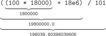
Notice that Python correctly performs exponentiation before multiplication, as in standard arithmetic. These operator precedence rules, all of which conform to standard arithmetic, are summarized in Table 2.1. As you might expect, you can override the default precedence with parentheses. For example, suppose we wanted to find the average salary at a retail company employing 100 salespeople with salaries of $18,000 per year and one CEO with a salary of $18 million:
>>> ((100 * 18000) + 18e6) / 101
196039.60396039605
In this case, we needed parentheses around (100 * 18000) + 18e6 to compute the total salaries before dividing by the number of employees. However, we also included parentheses around 100 * 18000 for clarity.
We should also point out that the answers in the previous two examples were floating point numbers, even though some of the numbers in the original expression were integers. When Python performs arithmetic with an integer and a floating point number, it first converts the integer to floating point. For example, in the last expression, (100 * 18000) evaluates to the integer value 1800000. Then 1800000 is added to the floating point number 18e6. Since these two operands are of different types, 1800000 is converted to the floating point equivalent 1800000.0 before adding. Then the result is the floating point value 19800000.0. Finally, 19800000.0 is divided by the integer 101. Again, 101 is converted to floating point first, so the actual division operation is 19800000.0 / 101.0, giving the final answer. This process is also depicted below.
In most cases, this works exactly as we would expect, and we do not need to think about this automatic conversion taking place.
Complex numbers
Although we will not use them in this book, it is worth pointing out that Python can also handle complex numbers. A complex number has both a real part and an imaginary part involving the imaginary unit i, which has the property that i2 = –1. In Python, a complex number like 3.2 + 2i is represented as 3.2 + 2j.(The letter j is used instead of i because in some fields, such as electrical engineering, i has another well-established meaning that could lead to ambiguities.) Most of the normal arithmetic operators work on complex numbers as well. For example,
>>> (5 + 4j) + (-4 + -3.1j)
(1+0.8999999999999999j)
>>> (23 + 6j) / (1 + 2j)
(7-8j)
>>> (1 + 2j) ** 2
(-3+4j)
>>> 1j ** 2
(-1+0j)
The last example illustrates the definition of i: i2 = –1.
Exercises
Use the Python interpreter to answer the following questions. Where appropriate, provide both the answer and the Python expression you used to get it.
2.2.1. The Library of Congress stores its holdings on 838 miles of shelves. Assuming an average book is one inch thick, how many books would this hold? (There are 5,280 feet in one mile.)
2.2.2. If I gave you a nickel and promised to double the amount you have every hour for the next 24, how much money would you have at the end? What if I only increased the amount by 50% each hour, how much would you have? Use exponentiation to compute these quantities.
2.2.3. The Library of Congress stores its holdings on 838 miles of shelves. How many round trips is this between Granville, Ohio and Columbus, Ohio?
2.2.4. The earth is estimated to be 4.54 billion years old. The oldest known fossils of anatomically modern humans are about 200,000 years old. What fraction of the earth’s existence have humans been around? Use Python’s scientific notation to compute this.
2.2.5. If you counted at an average pace of one number per second, how many years would it take you to count to 4.54 billion? Use Python’s scientific notation to compute this.
2.2.6. Suppose the internal clock in a modern computer can “count” about 2.8 billion ticks per second. How long would it take such a computer to tick 4.54 billion times?
2.2.7. A hard drive in a computer can hold about a terabyte (240 bytes) of information. An average song requires about 8 megabytes (8 × 220 bytes). How many songs can the hard drive hold?
2.2.8. What is the value of each of the following Python expressions? Make sure you understand why in each case.
15 * 3 - 215 - 3 * 215 * 3 // 215 * 3 / 215 * 3 % 215 * 3 / 2e0
2.3 WHAT’S IN A NAME?
Both in algorithms and in programs, a name associated with a value is called a variable. For example, in computing the volume of a sphere (using the formula V = (4/3)πr3), we might use a variable to refer to the sphere’s radius and another variable to refer to the (approximate) value of π:
>>> pi = 3.14159
>>> radius = 10
>>> (4 / 3) * pi * (radius ** 3)
4188.786666666666
The equal sign (=) is called the assignment operator because it is used to assign values to names. In this example, we assigned the value 3.14159 to the name pi and we assigned the value 10 to the name radius. It is convenient to think of variable names as “Sticky notes”1 attached to locations in the computer’s memory.
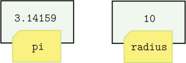
Recall from Section 1.4 that numbers are stored in cells in a computer’s memory. These cells are analogous to post office boxes; the cell’s address is like the number on the post office box and the value stored in the cell is like the box’s content. In the picture above, each rectangle containing a number represents a memory cell. A variable name is a reference to a particular cell, analogous to a Sticky note with a name on it on a post office box. In this picture, the name pi refers to the cell containing the value 3.14159 and the name radius refers to the cell containing the value 10. We do not actually know the addresses of each of these memory cells, but there is no reason for us to because we will always refer to them by a variable name.
As with a sticky note, a value can be easily reassigned to a different name at a later time. For example, if we now assign a different value to the name radius, the radius Sticky note in the picture moves to a different value.
>>> radius = 17

After the reassignment, a reference to a different memory cell containing the value 17 is assigned radius. The value 10 may briefly remain in memory without a name attached to it, but since we can no longer access that value without a reference to it, the Python “garbage collection” mechanism will soon free up the memory that it occupies.
Naming values serves three important purposes. First, assigning oft-used values to descriptive names can make our algorithms much easier to understand. For example, if we were writing an algorithm to model competition between two species, such as wolves and moose (as in Project 4.4), using names for the birth rates of the two species, like birthRateMoose and birthRateWolves, rather than unlabeled values, like 0.5 and 0.005, makes the algorithm much easier to read. Second, as we will see in Section 3.5, naming inputs will allow us to generalize algorithms so that, instead of being tied to one particular input, they work for a variety of possible inputs. Third, names will serve as labels for computed values that we wish to use later, obviating the need to compute them again at that time.
Notice that we are using descriptive names, not just single letters, as is the convention in algebra. As noted above, using descriptive names is always important when you are writing programs because it makes your work more accessible to others. In the “real world,” programming is almost always a collaborative endeavor, so it is important for others to be able to understand your intentions. Sometimes assigning an intermediate computation to a descriptive name, even if not required, can improve readability.
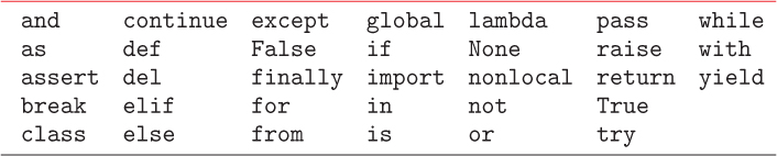
Names in Python can be any sequence of characters drawn from letters, digits, and the underscore (_) character, but they may not start with a digit. You also cannot use any of Python’s keywords, shown in Table 2.2. Keywords are elements of the Python language that have predefined meanings. We saw a few of these already in the snippets of Python code in Chapter 1 (def, for, in, and return), and we will encounter most of the others as we progress through this book.
Let’s try breaking some of these naming rules to see what happens.
>>> 49ers = 50
SyntaxError: invalid token
A syntax error indicates a violation of the syntax, or grammar, of the Python language. It is normal for novice programmers to encounter many, many syntax errors; it is part of the learning process. Most of the time, it will be immediately obvious what you did wrong, you will fix the mistake, and move on. Other times, you will need to look harder to discover the problem but, with practice, these instances too will become easier to diagnose. In this case, “invalid token” means that we have mistakenly used a name that starts with a digit. Token is a technical term that refers to any group of characters that the interpreter considers meaningful; in this case, it just refers to the name we chose.
Next, try this one.
>>> my-age = 21
SyntaxError: can't assign to operator
This syntax error is referring to the dash/hyphen/minus sign symbol (-) that we have in our name. Python interprets the symbol as the minus operator, which is why it is not allowed in names. Instead, we can use the underscore (_) character (i.e., my_age) or vary the capitalization (i.e., myAge) to distinguish the two words in the name.
In addition to assigning constant values to names, we can assign names to the results of whole computations.
>>> volume = (4 / 3) * pi * (radius ** 3)
When you assign values to names in the Python shell, the shell does not offer any feedback. But you can view the value assigned to a variable by simply typing its name.
>>> volume
20579.50889333333
So we see that we have assigned the value 20579.50889333333 to the name volume, as depicted below. (The values assigned to pi and radius are unchanged.)

Alternatively, you can display a value using print, followed by the value you wish to see in parentheses. Soon, when we begin to write programs outside of the shell, print will be the only way to display values.
>>> print(volume)
20579.50889333333
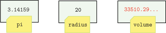
Now let’s change the value of radius again:
>>> radius = 20

Since the value of volume was based on the value of radius, it makes sense to check whether the value of volume has also changed. Try it:
>>> volume
20579.50889333333
What’s going on here? While the value assigned to radius has changed, the value assigned to volume has not. This example demonstrates that assignment is a onetime event; Python does not “remember” how the value of volume was computed. Put another way, an assignment is not creating an equivalence between a name and a computation. Rather, it performs the computation on the righthand side of the assignment operator only when the assignment happens, and then assigns the result to the name on the lefthand side. That value remains assigned to the name until it is explicitly assigned some other value or it ceases to exist. To compute a new value for volume based on the new value of radius, we would need to perform the volume computation again.
>>> volume = (4 / 3) * pi * (radius ** 3)
>>> volume
33510.29333333333
Now the value assigned to volume has changed, due to the explicit assignment statement above.
Let’s try another example. The formula for computing North American wind chill temperatures, in degrees Celsius, is
W = 13.12 + 0.6215t + (0.3965t – 11.37) v0.16
where t is the ambient temperature in degrees Celsius and v is the wind speed in km/h.2 To compute the wind chill for a temperature of –3° C and wind speed of 13 km/h, we will first assign the temperature and wind speed to two variables:
>>> temp = -3
>>> wind = 13
Then we type in the formula in Python, assigning the result to the name chill.
>>> chill = 13.12 + 0.6215 * temp + (0.3965 * temp - 11.37) * wind**0.16
>>> chill
-7.676796032159553
Notice once again that changing temp does not change chill:
>>> temp = 4.0
>>> chill
-7.676796032159553
To recompute the value of chill with the new temperature, we need to re-enter the entire formula above, which will now use the new value assigned to temp.
>>> chill = 13.12 + 0.6215 * temp + (0.3965 * temp - 11.37) * wind**0.16
>>> chill
0.8575160333891443
This process is, of course, very tedious and error-prone. Fortunately, there is a much better way to define such computations, as we will see in Section 3.5.
It is very important to realize that, despite the use of the equals sign, assignment is not the same as equality. In other words, when we execute an assignment statement like temp = 4.0, we are not asserting that temp and 4.0 are equivalent. Instead, we are assigning a value to a name in two steps:
Evaluate the expression on the righthand side of the assignment operator.
Assign the resulting value to the name on the lefthand side of the assignment operator.
For example, consider the following assignment statements:
>>> radius = 20
>>> radius = radius + 1
If the equals sign denoted equality, then the second statement would not make any sense! However, if we interpret the statement using the two-step process, it is perfectly reasonable. First, we evaluate the expression on the righthand side, ignoring the lefthand side entirely. Since, at this moment, the value 20 is assigned to radius, the righthand side evaluates to 21. Second, we assign the value 21 to the name radius. So this statement has added 1 to the current value of radius, an operation we refer to as an increment. To verify that this is what happened, check the value of radius:
>>> radius
21
What if we had not assigned a value to radius before we tried to increment it? To find out, we have to use a name that has not yet been assigned anything.
>>> trythis = trythis + 1
NameError: name 'trythis' is not defined
This name error occurred because, when the Python interpreter tried to evaluate the righthand side of the assignment, it found that trythis was not assigned a value, i.e., it was not defined. So we need to make sure that we first define any variable that we try to increment. This sounds obvious but, in the context of some larger programs later on, it might be easy to forget.
Let’s look at one more example. Suppose we want to increment the number of minutes displayed on a digital clock. To initialize the minutes count and increment the value, we essentially copy what we did above.
>>> minutes = 0
>>> minutes = minutes + 1
>>> minutes
1
>>> minutes = minutes + 1
>>> minutes
2
But incrementing is not going to work properly when minutes reaches 59, and we need the value of minutes to wrap around to 0 again. The solution lies with the modulo operator: if we mod the incremented value by 60 each time, we will get exactly the behavior we want. We can see what happens if we reset minutes to 58 and increment a few times:
>>> minutes = 58
>>> minutes = (minutes + 1) % 60
>>> minutes
59
>>> minutes = (minutes + 1) % 60
>>> minutes
0
>>> minutes = (minutes + 1) % 60
>>> minutes
1
When minutes is between 0 and 58, (minutes + 1) % 60 gives the same result as minutes + 1 because minutes + 1 is less than 60. But when minutes is 59, (minutes + 1) % 60 equals 60 % 60, which is 0. This example illustrates why arithmetic using the modulo operator, formally called modular arithmetic, is often also called “clock arithmetic.”
Exercises
Use the Python interpreter to answer the following questions. Where appropriate, provide both the answer and the Python expression you used to get it.
2.3.1. Every cell in the human body contains about 6 billion base pairs of DNA (3 billion in each set of 23 chromosomes). The distance between each base pair is about 3.4 angstroms (3.4 × 10⁻¹⁰ meters). Uncoiled and stretched, how long is the DNA in a single human cell? There are about 50 trillion cells in the human body. If you stretched out all of the DNA in the human body end to end, how long would it be? How many round trips to the sun is this? The distance to the sun is about 149,598,000 kilometers. Write Python statements to compute the answer to each of these three questions. Assign variables to hold each of the values so that you can reuse them to answer subsequent questions.
2.3.2. Set a variable named radius to have the value 10. Using the formula for the area of a circle (A = πr2), assign to a new variable named area the area of a circle with radius equal to your variable radius. (The number 10 should not appear in the formula.)
2.3.3. Now change the value of radius to 15. What is the value of area now? Why?
2.3.4. Suppose we wanted to swap the values of two variables named x and y. Why doesn’t the following work? Show a method that does work.
x = y
y = x
2.3.5. What are the values of x and y at the end of the following? Make sure you understand why this is the case.
x = 12.0
y = 2 * x
x = 6
2.3.6. What is the value of x at the end of the following? Make sure you understand why this is the case.
x = 0
x = x + 1
x = x + 1
x = x + 1
2.3.7. What are the values of x and y at the end of the following? Make sure you understand why this is the case.
x = 12.0
y = 6
y = y * x
2.3.8. Given a variable x that refers to an integer value, show how to extract the individual digits in the ones, tens and hundreds places. (Use the // and % operators.)
2.4 USING FUNCTIONS
A programming language like Python provides a rich set of functional abstractions that enable us to solve a wide variety of interesting problems. Variable names and arithmetic operators like ** are simple examples of this. Variable names allow us to easily refer to computation results without having to remember their exact values (e.g., volume in place of 33510.29333333333) and operators like ** allow us to perform more complex operations without explicitly specifying how (e.g., power notation in place of a more explicit algorithm that repeatedly multiplies).
In addition to the standard arithmetic operators, Python offers several more complex mathematical functions, each of which is itself another functional abstraction. A function takes one or more inputs, called arguments, and produces an output from them. You have probably seen mathematical functions like f(x) = x2 + 3 before. In this case, f is the name of the function, x is the single argument, and f(x) represents the output. The output is computed from the input (i.e., argument) by a simple algorithm represented on the righthand side of the equals sign. In this case, the algorithm is “square the input and add 3.” If we substitute x with a specific input value, then the algorithm produces a specific output value. For example, if x is 4, then the output is f(4) = 42 + 3 = 19, as illustrated below.

Does this look familiar? Like the example problems in Figure 1.1 (at the beginning of Chapter 1), a mathematical function has an input, an output, and an algorithm that computes the output from the input. So a mathematical function is another type of functional abstraction.
Built-in functions
As we suggested above, in a programming language, functional abstractions are also implemented as functions. In Chapter 3, we will learn how to define our own functions to implement a variety of functional abstractions, most of which are much richer than simple mathematical functions. In this section, we will set the stage by looking at how to use some of Python’s built-in functions. Perhaps the simplest of these is the Python function abs, which outputs the absolute value (i.e., magnitude) of its argument.
>>> result2 = abs(-5.0)
>>> result2
5.0
On the righthand side of the assignment statement above is a function call, also called a function invocation. In this case, the abs function is being called with argument -5.0. The function call executes the (hidden) algorithm associated with the abs function, and abs(-5.0) evaluates to the output of the function, in this case, 5.0. The output of the function is also called the function’s return value. Equivalently, we say that the function returns its output value. The return value of the function call, in this case 5.0, is then assigned to the variable name result2.
Two other helpful functions are float and int. The float function converts its argument to a floating point number, if it is not already.
>>> float(3)
3.0
>>> float(2.718)
2.718
The int function converts its argument to an integer by truncating it, i.e., removing the fractional part to the right of the decimal point. For example,
>>> int(2.718)
2
>>> int(-1.618)
-1
Recall the wind chill computation from Section 2.3:
>>> temp = -3
>>> wind = 13
>>> chill = 13.12 + 0.6215 * temp + (0.3965 * temp - 11.37) * wind**0.16
>>> chill
-7.676796032159553
Normally, we would want to truncate or round the final wind chill temperature to an integer. (It would be surprising to hear the local television meteorologist tell us, “the expected wind chill will be –7.676796032159553° C today.”) We can easily compute the truncated wind chill with
>>> truncChill = int(chill)
>>> truncChill
-7
There is also a round function that we can use to round the temperature instead.
>>> roundChill = round(chill)
>>> roundChill
-8
Alternatively, if we do not need to retain the original value of chill, we can simply assign the modified value to the name chill:
>>> chill = round(chill)
>>> chill
-8
Function arguments can be more complex than just single constants and variables; they can be anything that evaluates to a value. For example, if we want to convert the wind chill above to Fahrenheit and then round the result, we can do so like this:
>>> round(chill * 9/5 + 32)
18
The expression in parentheses is evaluated first, and then the result of this expression is used as the argument to the round function.
Not all functions output something. For example, the print function, which simply prints its arguments to the screen, does not. For example, try this:
>>> x = print(chill)
-8
>>> print(x)
None
The variable x was assigned whatever the print function returned, which is different from what it printed. When we print x, we see that it was assigned something called None. None is a Python keyword that essentially represents “nothing.” Any function that does not define a return value itself returns None by default. We will see this again shortly when we learn how to define our own functions.
Strings
As in the first “Hello world!” program, we often use the print function to print text:
>>> print('I do not like green eggs and ham.')
I do not like green eggs and ham.
The sentence in quotes is called a string. A string is simply text, a sequence of characters, enclosed in either single (') or double quotes ("). The print function prints the characters inside the quotation marks to the screen. The print function can actually take several arguments, separated by commas:
>>> print('The wind chill is', chill, 'degrees Celsius.')
The wind chill is -8 degrees Celsius.
The first and last arguments are strings, and the second is the variable we defined above. You will notice that a space is inserted between arguments, and there are no quotes around the variable name chill.
Reflection 2.2 Why do you think quotation marks are necessary around strings? What error do you think would result from typing the following instead? (Try it.)
>>> print(The expected wind chill is, chill, degrees Celsius.)
The quotation marks are necessary because otherwise Python has no way to distinguish text from a variable or function name. Without the quotation marks, the Python interpreter will try to make sense of each argument inside the parentheses, assuming that each word is a variable or function name, or a reserved word in the Python language. Since this sequence of words does not follow the syntax of the language, and most of these names are not defined, the interpreter will print an error.
String values can also be assigned to variables and manipulated with the + and * operators, but the operators have different meanings. The + operator concatenates two strings into one longer string. For example,
>>> first = 'Monty'
>>> last = 'Python'
>>> name = first + last
>>> print(name)
MontyPython
To insert a space between the first and last names, we can use another + operator:
>>> name = first + ' ' + last
>>> print(name)
Monty Python
Alternatively, if we just wanted to print the full name, we could have bypassed the name variable altogether.
>>> print(first + ' ' + last)
Monty Python
Reflection 2.3 Why do we not want quotes around first and last in the statement above? What would happen if we did use quotes?
Placing quotes around first and last would cause Python to interpret them literally as strings, rather than as variables:
>>> print('first' + ' ' + 'last')
first last
Applied to strings, the * operator becomes the repetition operator, which repeats a string some number of times. The operand on the left side of the repetition operator is a string and the operand on the right side is an integer that indicates the number of times to repeat the string.
>>> last * 4
'PythonPythonPythonPython'
>>> print(first + ' ' * 10 + last)
Monty          Python
We can also interactively query for string input in our programs with the input function. The input function takes a string prompt as an argument and returns a string value that is typed in response. For example, the following statement prompts for your name and prints a greeting.
>>> name = input('What is your name? ')
What is your name? George
>>> print('Howdy,', name, '!')
Howdy, George !
The call to the input function above prints the string 'What is your name? ' and then waits. After you type something (above, we typed George, shown in red) and hit Return, the text that we typed is returned by the input function and assigned to the variable called name. The value of name is then used in the print function.
Reflection 2.4 How can we use the + operator to avoid the inserted space before the exclamation point above?
To avoid the space, we can construct the string that we want to print using the concatenation operator instead of allowing the print function to insert spaces between the arguments:
>>> print('Howdy, ' + name + '!')
Howdy, George!
If we want to input a numerical value, we need to convert the string returned by the input function to an integer or float, using the int or float function, before we can use it as a number. For example, the following statements prompt for your age, and then print the number of days you have been alive.
>>> text = input('How old are you? ')
How old are you? 18
>>> age = int(text)
>>> print('You have been alive for', age * 365, 'days!')
You have been alive for 6570 days!
In the response to the prompt above, we typed 18 (shown in red). Then the input function assigned what we typed to the variable text as a string, in this case '18' (notice the quotes). Then, using the int function, the string is converted to the integer value 18 (no quotes) and assigned to the variable age. Now that age is a numerical value, it can be used in the arithmetic expression age * 365.
Reflection 2.5 Type the statements above again, omitting age = int(text):
>>> text = input('How old are you? ')
How old are you? 18
>>> print('You have been alive for', text * 365, 'days!')
What happened? Why?
Because the value of text is a string rather than an integer, the * operator was interpreted as the repetition operator instead!
Sometimes we want to perform conversions in the other direction, from a numerical value to a string. For example, if we printed the number of days in the following form instead, it would be nice to remove the space between the number of days and the period.
>>> print('The number of days in your life is', age * 365, '.')
The number of days in your life is 6570 .
But the following will not work because we cannot concatenate the numerical value age * 365 with the string '.'.
>>> print('The number of days in your life is', age * 365 + '.')
TypeError: unsupported operand type(s) for +: 'int' and 'str'
To make this work, we need to first convert age * 365 to a string with the str function:
>>> print('The number of days in your life is', str(age * 365) + '.')
The number of days in your life is 6570.
Assume the value 18 is assigned to age, then the str function converts the integer value 6570 to the string '6570' before concatenating it to '.'.
For a final, slightly more involved, example here is how we could prompt for a temperature and wind speed with which to compute the current wind chill.
>>> text = input('Temperature: ')
Temperature: 2.3
>>> temp = float(text)
>>> text = input('Wind speed: ')
Wind speed: 17.5
>>> wind = float(text)
>>> chill = 13.12 + 0.6215 * temp + (0.3965 * temp - 11.37) * wind**0.16
>>> chill = round(chill)
>>> print('The wind chill is', chill, 'degrees Celsius.')
The wind chill is -2 degrees Celsius.
Reflection 2.6 Why do we use float above instead of int? Replace one of the calls to float with a call to int, and then enter a floating point value (like 2.3). What happens and why?
>>> text = input('Temperature: ')
Temperature: 2.3
>>> temp = int(text)
Modules
In Python, there are many more mathematical functions available in a module named math. A module is an existing Python program that contains predefined values and functions that you can use. To access the contents of a module, we use the import keyword. To access the math module, type:
>>> import math
After a module has been imported, we can access the functions in the module by preceding the name of the function we want with the name of the module, separated by a period (.). For example, to take the square root of 5, we can use the square root function math.sqrt:
>>> math.sqrt(5)
2.23606797749979
Other commonly used functions from the math module are listed in Appendix B.1. The math module also contains two commonly used constants: pi and e. Our volume computation earlier would have been more accurately computed with:
>>> radius = 20
>>> volume = (4 / 3) * math.pi * (radius ** 3)
>>> volume
33510.32163829113
Notice that, since pi and e are variable names, not functions, there are no parentheses after their names.
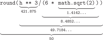
Function calls can also be used in longer expressions, and as arguments of other functions. In this case, it is useful to think about a function call as equivalent to the value that it returns. For example, we can use the math.sqrt function in the computation of the volume of a tetrahedron with edge length h = 7.5, using the formula .
>>> h = 7.5
>>> volume = h ** 3 / (6 * math.sqrt(2))
>>> volume
49.71844555217912
In the parentheses, the value of math.sqrt(2) is computed first, and then multiplied by 6. Finally, h ** 3 is divided by this result, and the answer is assigned to volume. If we want the rounded volume, we can use the entire volume computation as the argument to the round function:
>>> volume = round(h ** 3 / (6 * math.sqrt(2)))
>>> volume
50
We illustrate below the complete sequence of events in this evaluation:
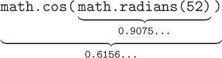
Now suppose we wanted to find the cosine of a 52° angle. We can use the math.cos function to compute the cosine, but the Python trigonometric functions expect their arguments to be in radians instead of degrees. (360 degrees is equivalent to 2π radians.) Fortunately, the math module provides a function named radians that converts degrees to radians. So we can find the cosine of a 52° angle like this:
>>> math.cos(math.radians(52))
0.6156614753256583
The function call math.radians(52) is evaluated first, giving the equivalent of 52° in radians, and this result is used as the argument to the math.cos function:
Finally, we note that, if you need to compute with complex numbers, you will want to use the cmath module instead of math. The names of the functions in the two modules are largely the same, but the versions in the cmath module understand complex numbers. For example, attempting to find the square root of a negative number using math.sqrt will result in an error:
>>> math.sqrt(-1)
ValueError: math domain error
This value error indicates that -1 is outside the domain of values for the math.sqrt function. On the other hand, calling the cmath.sqrt function to find returns the value of i:
>>> import cmath
>>> cmath.sqrt(-1)
1j
Exercises
Use the Python interpreter to answer the following questions. Where appropriate, provide both the answer and the Python expression you used to get it.
2.4.1. Try taking the absolute value of both –8 and –8.0. What do you notice?
2.4.2. Find the area of a circle with radius 10. Use the value of π from the math module.
2.4.3. The geometric mean of two numbers is the square root of their product. Find the geometric mean of 18 and 31.
2.4.4. Suppose you have P dollars in a savings account that will pay interest rate r, compounded n times per year. After t years, you will have
dollars in your account. If the interest were compounded continuously (i.e., with n approaching infinity), you would instead have
Pert
dollars after t years, where e is Euler’s number, the base of the natural logarithm. Suppose you have P = $10,000 in an account paying 1% interest (r = 0.01), compounding monthly. How much money will you have after t = 10 years? How much more money would you have after 10 years if the interest were compounded continuously instead? (Use the math.exp function.)
2.4.5. Show how you can use the int function to truncate any positive floating point number x to two places to the right of the decimal point. In other words, you want to truncate a number like 3.1415926 to 3.14. Your expression should work with any value of x.
2.4.6. Show how you can use the int function to find the fractional part of any positive floating point number. For example, if the value 3.14 is assigned to x, you want to output 0.14. Your expression should work with any value of x.
2.4.7. The well-known quadratic formula, shown below, gives solutions to the quadratic equation ax2 + bx + c = 0.
Show how you can use this formula to compute the two solutions to the equation 3x2 + 4x – 5 = 0.
2.4.8. Suppose we have two points (x1, y1) and (x2, y2). The distance between them is equal to
Show how to compute this in Python. Make sure you test your answer with real values.
2.4.9. A parallelepiped is a three-dimensional box in which the six sides are parallelograms. The volume of a parallelepiped is
where a, b, and c are the edge lengths, and x, y, and z are the angles between the edges, in radians. Show how to compute this in Python. Make sure you test your answer with real values.
2.4.10. Repeat the previous exercise, but now assume that the angles are given to you in degrees.
2.4.11. Repeat Exercise 2.4.4, but prompt for each of the four values first using the input function, and then print the result.
2.4.12. Repeat Exercise 2.4.7, but prompt for each of the values of a, b, and c first using the input function, and then print the results.
2.4.13. The following program implements a Mad Lib.
adj1 = input('Adjective: ')
noun1 = input('Noun: ')
noun2 = input('Noun: ')
adj2 = input('Adjective: ')
noun3 = input('Noun: ')

print('How to Throw a Party')
print()
print('If you are looking for a/an', adj1, 'way to')
print('celebrate your love of', noun1 + ', how about a')
print(noun2 + '-themed costume party? Start by')
print('sending invitations encoded in', adj2, 'format')
print('giving directions to the location of your', noun3 + '.')
Write your own Mad Lib program, requiring at least five parts of speech to insert. (You can download the program above from the book web site to get you started.)
*2.5 BINARY ARITHMETIC
Recall from Section 1.4 that numbers are stored in a computer’s memory in binary. Therefore, computers must also perform arithmetic in binary. In this section, we will briefly explore how binary addition works.
Although it may be unfamiliar, binary addition is actually much easier than decimal addition since there are only three basic binary addition facts: 0 + 0 = 0, 0 + 1 = 1 + 0 = 1, and 1 + 1 = 10. (Note that this is 10 in binary, which has the value 2 in decimal.) With these basic facts, we can add any two arbitrarily long binary numbers using the same right-to-left algorithm that we all learned in elementary school.
For example, let’s add the binary numbers 1110 and 0111. Starting on the right, we add the last column: 0 + 1 = 1.

In the next column, we have 1 + 1 = 10. Since the answer contains more than one bit, we carry the 1.

In the next column, we have 1 + 1 = 10 again, but with a carry bit as well. Adding in the carry, we have 10 + 1 = 11 (or 2 + 1 = 3 in decimal). So the answer for the column is 1, with a carry of 1.
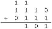
Finally, in the leftmost column, with the carry, we have 1 + 0 + 1 = 10. We write the 0 and carry the 1, and we are done.
We can easily check our work by converting everything to decimal. The top number in decimal is 8 + 4 + 2 + 0 = 14 and the bottom number in decimal is 0 + 4 + 2 + 1 = 7. Our answer in decimal is 16 + 4 + 1 = 21. Sure enough, 14 + 7 = 21.
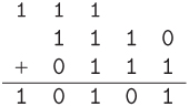
Finite precision
Although Python integers can store arbitrarily large values, this is not true at the machine language level. In other words, Python integers are another abstraction built atop the native capabilities of the computer. At the machine language level (and in most other programming langauges), every integer is stored in a fixed amount of memory, usually four bytes (32 bits). This is another example of finite precision, and it means that sometimes the result of an arithmetic operation is too large to fit.
We can illustrate this by revisiting the previous problem, but assuming that we only have four bits in which to store each integer. When we add the four-bit integers 1110 and 0111, we arrived at a sum, 10101, that requires five bits to be represented. When a computer encounters this situation, it simply discards the leftmost bit. In our example, this would result in an incorrect answer of 0101, which is 5 in decimal. Fortunately, there are ways to detect when this happens, which we leave to you to discover as an exercise.
Negative integers
We assumed above that the integers we were adding were positive, or, in programming terminology, unsigned. But of course computers must also be able to handle arithmetic with signed integers, both positive and negative.
Everything, even a negative sign, must be stored in a computer in binary. One option for representing negative integers is to simply reserve one bit in a number to represent the sign, say 0 for positive and 1 for negative. For example, if we store every number with eight bits and reserve the first (leftmost) bit for the sign, then 00110011 would represent 51 and 10110011 would represent –51. This approach is known as sign and magnitude notation. The problem with this approach is that the computer then has to detect whether a number is negative and handle it specially when doing arithmetic.
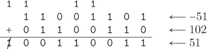
For example, suppose we wanted to add –51 and 102 in sign and magnitude notation. In this notation, –51 is 10110011 and 102 is 01100110. First, we notice that 10110011 is negative because it has 1 as its leftmost bit and 01100110 is positive because it has 0 as its leftmost bit. So we need to subtract positive 51 from 102:

Borrowing in binary works the same way as in decimal, except that we borrow a 2 (10 in binary) instead of a 10. Finally, we leave the sign of the result as positive because the largest operand was positive.
To avoid these complications, computers use a clever representation called two’s complement notation. Integers stored in two’s complement notation can be added directly, regardless of their sign. The leftmost bit is also the sign bit in two’s complement notation, and positive numbers are stored in the normal way, with leading zeros if necessary to fill out the number of bits allocated to an integer. To convert a positive number to its negative equivalent, we invert every bit to the left of the rightmost 1. For example, since 51 is represented in eight bits as 00110011, –51 is represented as 11001101. Since 4 is represented in eight bits as 00000100, –4 is represented as 11111100.
To illustrate how addition works in two’s complement notation, let’s once again add –51 and 102:
As a final step in the addition algorithm, we always disregard an extra carry bit. So, indeed, in two’s complement, –51 + 102 = 51.
Note that it is still possible to get an incorrect answer in two’s complement if the answer does not fit in the given number of bits. Some exercises below prompt you to investigate this further.
Designing an adder
Let’s look at how to an adder that takes in two single bit inputs and outputs a two bit answer. We will name the rightmost bit in the answer the “sum” and the leftmost bit the “carry.” So we want our abstract adder to look this:

The two single bit inputs enter on the left side, and the two outputs exit on the right side. Our goal is to replace the inside of this “black box” with an actual logic circuit that computes the two outputs from the two inputs.
The first step is to design a truth table that represents what the values of sum and carry should be for all of the possible input values:
a |
b |
carry |
sum |
0 |
0 |
0 |
0 |
0 |
1 |
0 |
1 |
1 |
0 |
0 |
1 |
1 |
1 |
1 |
0 |
Notice that the value of carry is 0, except for when a and b are both 1, i.e., when we are computing 1 + 1. Also, notice that, listed in this order (carry, sum), the two output bits can also be interpreted as a two bit sum: 0 + 0 = 00, 0 + 1 = 1, 1 + 0 = 1, and 1 + 1 = 10. (As in decimal, a leading 0 contributes nothing to the value of a number.)
Next, we need to create an equivalent Boolean expression for each of the two outputs in this truth table. We will start with the sum column. To convert this column to a Boolean expression, we look at the rows in which the output is 1. In this case, these are the second and third rows. The second row says that we want sum to be 1 when a is 0 and b is 1. The and in this sentence is important; in order for an and expression to be 1, both inputs must be 1. But, in this case, a is 0 so we need to flip it with not a. The b input is already 1, so we can leave it alone. Putting these two halves together, we have not a and b. Now the third row says that we want sum to be 1 when a is 1 and b is 0. Similarly, we can convert this to the Boolean expression a and not b.


Finally, let’s combine these two expressions into one expression for the sum column: taken together, these two rows are saying that sum is 1 if a is 0 and b is 1, or if a is 1 and b is 0. In other words, we need at least one of these two cases to be 1 for the sum column to be 1. This is just equivalent to (not a and b) or (a and not b). So this is the final Boolean expression for the sum column.
Now look at the carry column. The only row in which the carry bit is 1 says that we want carry to be 1 if a is 1 and b is 1. In other words, this is simply a and b. In fact, if you look at the entire carry column, you will notice that this column is the same as in the truth table for a and b. So, to compute the carry, we just compute a and b.

Implementing an adder
To implement our adder, we need physical devices that implement each of the binary operators. Figure 2.1(a) shows a simple electrical implementation of an and operator. Imagine that electricity is trying to flow from the positive terminal on the left to the negative terminal on the right and, if successful, light up the bulb. The binary inputs, a and b, are each implemented with a simple switch. When the switch is open, it represents a 0, and when the switch is closed, it represents a 1. The light bulb represents the output (off = 0 and on = 1). Notice that the bulb will only light up if both of the switches are closed (i.e., both of the inputs are 1). An or operator can be implemented in a similar way, represented in Figure 2.1(b). In this case, the bulb will light up if at least one of the switches is closed (i.e., if at least one of the inputs is 1).

Physical implementations of binary operators are called logic gates. It is interesting to note that, although modern gates are implemented electronically, they can be implemented in other ways as well. Enterprising inventors have implemented hydraulic and pneumatic gates, mechanical gates out of building blocks and sticks, optical gates, and recently, gates made from molecules of DNA.
Logic gates have standard, implementation-independent schematic representations, shown in Figure 2.2. Using these symbols, it is a straightforward matter to compose gates to create a logic circuit that is equivalent to any Boolean expression. For example, the expression not a and b would look like the following:
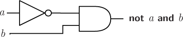
Both inputs a and b enter on the left. Input a enters a not gate before the and gate, so the top input to the and gate is not a and the bottom input is simply b. The single output of the circuit on the right leaves the and gate with value not a and b. In this way, logic circuits can be built to an arbitrary level of complexity to perform useful functions.
The circuit for the carry output of our adder is simply an and gate:

The circuit for the sum output is a bit more complicated:
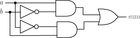
By convention, the solid black circles represent connections between “wires”; if there is no solid black circle at a crossing, this means that one wire is “floating” above the other and they do not touch. In this case, by virtue of the connections, the a input is flowing into both the top and gate and the bottom not gate, while the b input is flowing into both the top not gate and the bottom and gate. The top and gate outputs the value of a and not b and the bottom and gate outputs the value of not a and b. The or gate then outputs the result of oring these two values.
Finally, we can combine these two circuits into one grand adder circuit with two inputs and two outputs, to replace the “black box” adder we began with. The shaded box represents the “black box” that we are replacing.
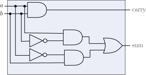
Notice that the values of both a and b are each now flowing into three different gates initially, and the two outputs are conceptually being computed in parallel. For example, suppose a is 0 and b is 1. The figure below shows how this information flows through the adder to arrive at the final output values.

In this way, the adder computes 0 + 1 = 1, with a carry of 0.
Exercises
2.5.1. Show how to add the unsigned binary numbers 001001 and 001101.
2.5.2. Show how to add the unsigned binary numbers 0001010 and 0101101.
2.5.3. Show how to add the unsigned binary numbers 1001 and 1101, assuming that all integers must be stored in four bits. Convert the binary values to decimal to determine if you arrived at the correct answer.
2.5.4. Show how to add the unsigned binary numbers 001010 and 101101, assuming that all integers must be stored in six bits. Convert the binary values to decimal to determine if you arrived at the correct answer.
2.5.5. Suppose you have a computer that stores unsigned integers in a fixed number of bits. If you have the computer add two unsigned integers, how can you tell if the answer is correct (without having access to the correct answer from some other source)? (Refer back to the unsigned addition example in the text.)
2.5.6. Show how to add the two’s complement binary numbers 0101 and 1101, assuming that all integers must be stored in four bits. Convert the binary values to decimal to determine if you arrived at the correct answer.
2.5.7. What is the largest positive integer that can be represented in four bits in two’s complement notation? What is the smallest negative number? (Think especially carefully about the second question.)
2.5.8. Show how to add the two’s complement binary numbers 1001 and 1101, assuming that all integers must be stored in four bits. Convert the binary values to decimal to determine if you arrived at the correct answer.
2.5.9. Show how to add the two’s complement binary numbers 001010 and 101101, assuming that all integers must be stored in six bits. Convert the binary values to decimal to determine if you arrived at the correct answer.
2.5.10. Suppose you have a computer that stores two’s complement integers in a fixed number of bits. If you have the computer add two two’s complement integers, how can you tell if the answer is correct (without having access to the correct answer from some other source)?
2.5.11. Subtraction can be implemented by adding the first operand to the two’s complement of the second operand. Using this algorithm, show how to subtract the two’s complement binary number 0101 from 1101. Convert the binary values to decimal to determine if you arrived at the correct answer.
2.5.12. Show how to subtract the two’s complement binary number 0011 from 0110. Convert the binary values to decimal to determine if you arrived at the correct answer.
2.5.13. Copy the completed adder circuit, and show, as we did above, how the two outputs (carry and sum) obtain their final values when the input a is 1 and the input b is 0.
2.5.14. Convert the Boolean expression not (a and b) to a logic circuit.
2.5.15. Convert the Boolean expression not a and not b to a logic circuit.
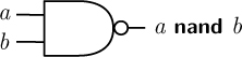
2.5.16. The single Boolean operator nand (short for “not and”) can replace all three traditional Boolean operators. The truth table and logic gate symbol for nand are shown below.
a |
b |
a nand b |
0 |
0 |
1 |
0 |
1 |
1 |
1 |
0 |
1 |
1 |
1 |
0 |
Show how you can create three logic circuits, using only nand gates, each of which is equivalent to one of the and, or, and not gates. (Hints: you can use constant inputs, e.g., inputs that are always 0 or 1, or have both inputs of a single gate be the same.)
2.6 SUMMARY
To learn how to write algorithms and programs, you have to dive right in! We started our introduction to programming in Python by performing simple computations on numbers. There are two numerical types in Python: integers and floating point numbers. Floating point numbers have a decimal point and sometimes behave differently than we expect due to their finite precision. Aside from these rounding errors, most arithmetic operators in Python behave as we would expect, except that there are two kinds of division: so-called true division and floor division.
We use descriptive variable names in our programs for two fundamental reasons. First, they make our code easier to understand. Second, they can “remember” our results for later so that they do not have to be recomputed. The assignment statement is used to assign values to variable names. Despite its use of the equals sign, using an assignment statement is not the same thing as saying that two things are equal. Instead, the assignment statement evaluates the expression on the righthand side of the equals sign first, and then assigns the result to the variable on the lefthand side.
Functional abstractions in Python are implemented as functions. Functions take arguments as input and then return a value as output. When used in an expression, it is useful to think of a function call as equivalent to the value that it returns. We used some of Python’s built-in functions, and the mathematical functions provided by the math module. In addition to numerical values, Python lets us print, input, and manipulate string values, which are sequences of characters enclosed in quotation marks.
Because everything in a computer is represented in binary notation, all of these operators and functions are really computed in binary, and then expressed to us in more convenient formats. As an example, we looked at how positive and negative integers are stored in a computer, and how two binary integers can be added together just by using the basic Boolean operators of and, or, and not.
In the next chapter, we will begin to write our own functions and incorporate them into longer programs. We will also explore Python’s “turtle graphics” module, which will allow us to draw pictures and visualize our data.
2.7 FURTHER DISCOVERY
The epigraph at the beginning of this chapter is from the great Donald Knuth [26]. When he was still in graduate school in the 1960’s Dr. Knuth began his life’s work, a multi-volume set of books titled, The Art of Computer Programming [24]. In 2011, he published the first part of Volume 4, and has plans to write seven volumes total. Although incomplete, this work was cited at the end of 1999 in American Scientist’s list of “100 or so Books that Shaped a Century of Science” [35]. Dr. Knuth also invented the typesetting program TEX, which was used to write this book. He is the recipient of many international awards, including the Turing Award, named after Alan Turing, which is considered to be the “Nobel Prize of computer science.”
Guido van Rossum is a Dutch computer programmer who invented the Python programming language. The assertion that Van Rossum was in a “slightly irreverent mood” when he named Python after the British comedy show is from the Foreword to Programming Python [29] by Mark Lutz. IDLE is an acronym for “Integrated DeveLopment Environment,” but is also considered to be a tribute to Eric Idle, one of the founders of Monty Python.
The “Hello world!” program is the traditional first program that everyone learns when starting out. See
http://en.wikipedia.org/wiki/Hello_world_program
for an interesting history.
As you continue to program in Python, it might be helpful to add the following web site containing Python documentation to your “favorites” list:
https://docs.python.org/3/index.html
There is also a list of links on the book web site, and references to commonly used classes and function in Appendix B.
1“Sticky note” is a registered trademark of the BIC Corporation.
2Technically, wind chill is only defined at or below 10° C and for wind speeds above 4.8 km/h.