
CHAPTER 12
Networks
Fred Jones of Peoria, sitting in a sidewalk cafe in Tunis and needing a light for his cigarette, asks the man at the next table for a match. They fall into conversation; the stranger is an Englishman who, it turns out, spent several months in Detroit studying the operation of an interchangeable-bottlecap factory. “I know it’s a foolish question,” says Jones, “but did you ever by any chance run into a fellow named Ben Arkadian? He’s an old friend of mine, manages a chain of supermarkets in Detroit...”
“Arkadian, Arkadian,” the Englishman mutters. “Why, upon my soul, I believe I do! Small chap, very energetic, raised merry hell with the factory over a shipment of defective bottlecaps.”
“No kidding!” Jones exclaims in amazement.
“Good lord, it’s a small world, isn’t it?”
Stanley Milgram
The Small-World Problem (1967)
WHAT do Facebook, food webs, the banking system, and our brains all have in common? They are all networks: systems of interconnected units that exchange information over the links between them. There are networks all around us: social networks, road networks, protein interaction networks, electrical transmission networks, the Internet, networks of seismic faults, terrorist networks, networks of political influence, transportation networks, and semantic networks, to name a few.
The continuous and dynamic local interactions in large networks such as these make them extraordinarily complex and hard to predict. Learning more about networks can help us combat disease, terrorism, and power outages. Realizations that some networks are emergent systems that develop global behaviors based on local interactions have improved our understanding of insect colonies, urban planning, and even our brains. Too little understanding of networks has had unfortunate consequences, such as when invasive species have been introduced into poorly understood ecological networks.
As with the other types of “big data,” we need computers and algorithms to understand large and complex networks. In this chapter, we will begin by discussing how we can represent networks in algorithms so that we can analyze them. Then we will develop an algorithm to find the distance between any two nodes in a network. Recent discoveries have shown that many real networks exhibit a “small-world property,” meaning that the average distance between nodes is relatively small. In later sections, we will computationally investigate the characteristics of small-world networks and their ramifications for solving real problems.

12.1 MODELING WITH GRAPHS
We model networks with a mathematical structure called a graph. A graph consists of a set of nodes (or vertices) and a set of links (or edges) that connect pairs of nodes. Nodes are usually drawn as circles (or another shape) and links are drawn as lines between them, as in Figure 12.1. If two nodes are connected by a link, we say they are adjacent. A graph is completely represented by its nodes and links. Although we often draw graphs to gain insight into their structure, the placement of the nodes and links on the page is arbitrary. In other words, there can be many different visual representations of the same graph. For example, all three of the graphs in Figure 12.1 are equivalent.
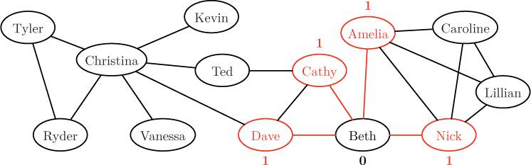
A social network (like Facebook or LinkedIn) can be represented by a graph in which the nodes are people and the links represent relationships (e.g., friends, connections, circles, followers). For example, in the social network in Figure 12.2, Caroline has three friends: Amelia, Lillian, and Nick. In a neural network, the nodes represent neurons and the links represent axons that transmit nerve impulses between the neurons. Figure 12.3 represents the interconnections between neurons in one of the simple neural networks that control digestion in the guts of arthropods. In a graph representing a power grid, like that in Figure 12.4, the nodes represent power stations and the links represent high-voltage transmission lines connecting them.
In an algorithm, a graph is usually represented in one of two ways. The first method is called an adjacency matrix. An adjacency matrix contains a row and a column for every node in the network. A one in a matrix entry represents a link between the nodes in the corresponding row and column. A zero means that there is no link. An adjacency matrix for the network in Figure 12.2 can be represented by the following table.


Figure 12.3 A model of the pyloric central pattern generator that controls stomach motion in lobsters.

Figure 12.4 The electrical transmission network in New Zealand. [58]
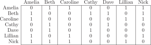
For example, the first row in the adjacency matrix indicates that Amelia is only connected to Beth, Caroline, Lillian, and Nick. In Python, we would represent this matrix with the following nested list.
graph = [[0, 1, 1, 0, 0, 1, 1],
         [1, 0, 0, 1, 1, 0, 1],
         [1, 0, 0, 0, 0, 1, 1],
         [0, 1, 0, 0, 1, 0, 0],
         [0, 1, 0, 1, 0, 0, 0],
         [1, 0, 1, 0, 0, 0, 1],
         [1, 1, 1, 0, 0, 1, 0]]

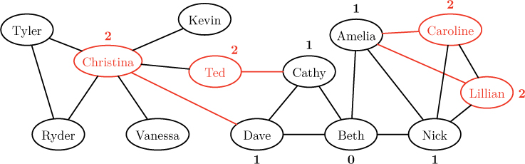
Figure 12.5 An expanded social network. The nodes and links in red are additions to the graph in Figure 12.2.
Although the nodes’ labels are not stored in the adjacency matrix itself, they could be stored separately as strings in a list. The index of each string in the list should equal the row and column of the corresponding node in the adjacency matrix.
Reflection 12.1 Create an adjacency matrix for the graph in Figure 12.1. (Remember that all three pictures depict the same graph.)
The alternative representation, which we will use in this chapter, is an adjacency list. An adjacency list, which is actually a collection of lists, contains, for each node, a list of nodes to which it is connected. In Python, an adjacency list can be stored as a dictionary. For the network in Figure 12.2, this would look like the following:
graph = {'Amelia': ['Beth', 'Caroline', 'Lillian', 'Nick'],
         'Beth': ['Amelia', 'Cathy', 'Dave', 'Nick'],
         'Caroline': ['Amelia', 'Lillian', 'Nick'],
         'Cathy': ['Beth', 'Dave'],
         'Dave': ['Beth', 'Cathy'],
         'Lillian': ['Amelia', 'Caroline', 'Nick'],
         'Nick': ['Amelia', 'Beth', 'Caroline', 'Lillian']}
Each key in this dictionary, a string, represents a node, and each corresponding value is a list of strings representing the nodes to which the key node is connected. Notice that, if two nodes are connected, that information is stored in both nodes’ lists. For example, there is a link connecting Amelia and Beth, so Beth is in Amelia’s list and Amelia is in Beth’s list.
Reflection 12.2 Create an adjacency list for the graph in Figure 12.1.
Making friends
Social networking sites often have an eerie ability to make good suggestions about who you should add to your list of “connections” or “friends.” One way they do this is by examining the connections of your connections (or “friends-of-friends”). For example, consider the expanded social network graph in Figure 12.5. Dave currently has only three friends. But his friends have an additional seven friends that an algorithm could suggest to Dave.
Reflection 12.3 Who are the seven friends-of-friends of Dave in Figure 12.5?
In graph terminology, the connections of a node are called the node’s neighborhood, and the size of a node’s neighborhood is called its degree. In the graph in Figure 12.5, Dave’s neighborhood contains Beth, Cathy and Christina, and therefore his degree is three.
Reflection 12.4 How can you compute the degree of a node from the graph’s adjacency matrix? What about from the graph’s adjacency list?
Once we have a network in an adjacency list, writing an algorithm to collect new friend suggestions is relatively easy. The function below iterates over the neighbors of the node for which we would like suggestions and then, for each of these neighbors, iterates over the neighbors’ neighbors.
 1 def friendsOfFriends(network, node):
 2     """Find new neighbors-of-neighbors of a node in a network.
 3
 4     Parameters:
 5         network: a graph represented by a dictionary
 6         node: a node in the network
 7
 8     Return value: a list of new neighbors-of-neighbors of node
 9     """
10
11     suggestions = [ ]
12     neighbors = network[node]
13     for neighbor in neighbors:                # neighbors of node
14         for neighbor2 in network[neighbor]:   # neighbors of neighbors
15             if neighbor2 != node and
16                neighbor2 not in neighbors and
17                neighbor2 not in suggestions:
18                 suggestions.append(neighbor2)
19     return suggestions
On line 12, network[node] is the list of nodes to which node is connected in the adjacency list named network. We assign this list to neighbors, and then iterate over it on line 13. On line 14, in the inner for loop, we then iterate over the list of each neighbors’ neighbors. In the if statement, we choose suggestions to be a list of unique neighbors-of-neighbors that are not the node itself or neighbors of the node.
Reflection 12.5 Look carefully at the three-part if statement in the function above. How does each part contribute to the desired characteristics of suggestions listed above?
Reflection 12.6 Insert the additional nodes and links from Figure 12.5 (in red) into the dictionary on Page 590. Then call the friendsOfFriends function with this graph to find new friend suggestions for Dave.
In the next section, we will design an algorithm to find paths to nodes that are farther away. The ability to compute the distance between nodes will also allow us to better characterize and understand large networks.
Exercises
12.1.1. Besides those presented in this section, describe three other examples of networks.
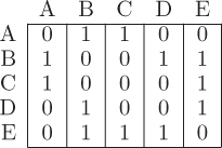
12.1.2. Draw the network represented by the following adjacency matrix.
12.1.3. Draw the network represented by the following adjacency list.
graph = {'A': ['C', 'D', 'F'],
          'B': ['C', 'E'],
          'C': ['A', 'B', 'D'],
          'D': ['A', 'C'],
          'E': ['B', 'F'],
          'F': ['A', 'E']}
12.1.4. Show how the following network would be represented in Python as
an adjacency matrix
an adjacency list

12.1.5. What is the neighborhood of each of the nodes in the network from Exercise 12.1.4?
12.1.6. What is the degree of each node in the network from Exercise 12.1.4? Which node(s) have the maximum degree?
12.1.7. Are the networks in each of the following pairs the same or different? Why?
(a) 
(b) 
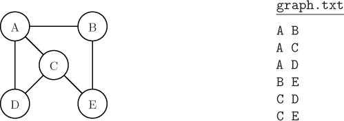
12.1.8. A graph can be represented in a file by listing one link per line, with each link represented by a pair of nodes. For example, the graph below is represented by the file on the right. Write a function that reads such a file and returns an adjacency list (as a dictionary) for the graph. Notice that, for each line A B in the file, your function will need to insert node B into the list of neighbors of A and insert node A into the list of neighbors of B.
12.1.9. In this chapter, we are generally assuming that all graphs are undirected, meaning that each link represents a mutual relationship between two nodes. For example, if there is a link between nodes A and B, then this means that A is friends with B and B is friends with A, or that one can travel from city A to city B and from city B to city A. However, the relationships between nodes in some networks are not mutual or do not exist in both directions. Such a network is more accurately represented by a directed graph (or digraph), in which links are directed from one node to another. In a picture, the directions are indicated arrows. For example, in the directed graph below, one can go directly from node A to node B, but not vice versa. However, one can go in both directions between nodes B and E.

- (a) Give three examples of networks that are better represented by a directed graph.
- (b) How would an adjacency list representation of a directed graph differ from that of an undirected graph?
- (c) Write a function that reads a file representing a directed graph (see the example above), and returns an adjacency list (as a dictionary) representing that directed graph.
12.1.10. Write a function that returns the maximum degree in a network represented by an adjacency list (dictionary).
12.1.11. Write a function that returns the average degree in a network represented by an adjacency list (dictionary).
12.2 SHORTEST PATHS
A sequence of links (or equivalently, linked nodes) between two nodes is called a path. A path with the minimum number of links is called a shortest path. For example, in Figure 12.5, a shortest path from Dave to Lillian starts with Dave, then visits Beth, then Nick, then Lillian. The distance between two nodes is the number of links on a shortest path between them. Because three links were crossed along the shortest path from Dave to Lillian, the distance between them is 3.
Computing the distance between two nodes is a fundamental problem in network analysis. In a transportation network, the distance between a source and destination gives the number of stops along the route. In an ecological network, the distance between two organisms may be a measure of how dependent one organism is upon the other. In a social network, the distance between two people is the number of introductions by friends that would be necessary for one person to meet the other.
Reflection 12.7 Are shortest paths always unique? Is there another shortest path between Dave and Lillian?
Yes, there is:
There may be many shortest paths between two nodes in a network, but in most applications we are concerned with just finding one.
Shortest paths can be computed using an algorithm called breadth-first search (BFS). A breadth-first search explores outward from a source node, first visiting all nodes with distance one from the source, then all nodes with distance two, etc., until it has visited every reachable node in the network. In other words, the BFS algorithm incrementally pushes its “frontier” of visited nodes outward from the source. When the algorithm finishes, it has computed the distances between the source node and every other node.
For example, suppose we wanted to discover the distance from Beth to every other person in the social network in Figure 12.5, reproduced below.
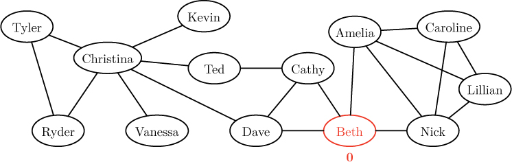
As indicated above, we begin by labeling Beth’s node with distance 0, signifying that there are zero links between the node and itself. Then, in the first round of the algorithm, we explore all neighbors of Beth, colored red below.
Since these nodes are one hop away from the source, we label them with distance 1. These nodes now comprise the “frontier” being explored by the algorithm. In the next round, we explore all unvisited neighbors of the nodes on this frontier, as shown below.
As indicated by the red links, Christina is visited from Dave, Ted is visited from Cathy, and both Caroline and Lillian are visited from Amelia. Notice that Caroline and Lillian could have been visited from Nick as well. The decision is arbitrary, depending, as we will see, on the order in which nodes are considered by the algorithm. Since all four of these nodes are neighbors of a node with distance 1, we label them with distance 2. Finally, in the third round, we visit all unvisited neighbors of the new frontier of nodes, as shown below.
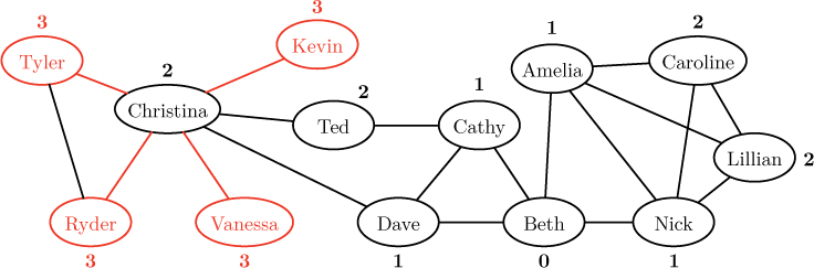
Since these newly visited nodes are all neighbors of a node labeled with distance 2, we label all of them with distance 3. At this point, all of the nodes have been visited, and the final label of each node gives its distance from the source.
Reflection 12.8 If you also studied the depth-first search algorithm in Section 10.5, compare and contrast that approach with breadth-first search.
In an algorithm, keeping track of the nodes on the current frontier could get complicated. The trick is to use a queue. A queue is a list in which items are always inserted at the end and deleted from the front. The insertion operation is called enqueue and the deletion operation is called dequeue.

Reflection 12.9 In Python, if we use a list named queue to implement a queue, how do we perform the enqueue and dequeue operations?
An enqueue operation is simply an append:
queue.append(item) # enqueue an item
And then a dequeue can be implemented by “popping” the front item from the list:
item = queue.pop(0) # dequeue an item
In the breadth-first search algorithm, we use a queue to remember those nodes on the “frontier” that have been visited, but from which the algorithm has not yet visited new nodes. When we are ready to visit the unvisited neighbors of a node on the frontier, we dequeue that node, and then enqueue the newly visited neighbors so that we can remember to explore outward from them later.
Reflection 12.10 Why can we not explore outward from these newly visited neighbors right away? Why do they need to be stored in the queue for later?
We need to wait because there may be nodes further ahead in the queue that have smaller distances from the source. For the algorithm to work correctly, we have to explore outward from these nodes first.
The following Python function implements the breadth-first search algorithm.
 1 def bfs(network, source):
 2     """Perform a breadth-first search on network, starting from source.
 3
 4     Parameters:
 5         network: a graph represented by a dictionary
 6         source: the node in network from which to start the BFS
 7
 8     Return value: a dictionary with distances from source to all nodes
 9     """
10
11     visited = { }
12     distance = { }
13     for node in network:
14         visited[node] = False
15         distance[node] = float('inf')
16     visited[source] = True
17     distance[source] = 0
18     queue = [source]
19     while queue != [ ]:
20         front = queue.pop(0)             # dequeue front node
21         for neighbor in network[front]:
22             if not visited[neighbor]:
23                 visited[neighbor] = True
24                 distance[neighbor] = distance[front] + 1
25                 queue.append(neighbor)   # enqueue visited node
26     return distance
The function maintains two dictionaries: visited keeps track of whether each node has been visited and distance keeps track of the distance from the source to each node. Lines 11–17 initialize the dictionaries. Every node, except the source, is marked as unvisited and assigned an initial distance of infinity (∞) because we do not yet know which nodes can be reached from the source. (The expression float('inf') creates a special value representing ∞ that is greater than every other floating point value.) The source is marked as visited and assigned distance zero. On line 18, the queue is initialized to contain just the source node. Then, while the queue is not empty, the algorithm repeatedly dequeues the front node (line 20), and explores all neighbors of this node (lines 21–25). If a neighbor has not yet been visited (line 22), it is marked as visited (line 23), assigned a distance that is one greater than the node from which it is being visited (line 24), and then enqueued (line 25). Once the queue is empty, we know that all reachable nodes have been visited, so we return the distance dictionary, which now contains the distance to each node.
Reflection 12.11 Call the bfs function with the graph that you created earlier, to find the distances from Beth to all other nodes.
Reflection 12.12 What does it mean if the bfs function returns a distance of ∞ for a node?
If the final distance is ∞, then the node must not have been visited by the algorithm, which means that there is no path to it from the source.
Reflection 12.13 If you just want the distance between two particular nodes, named source and dest, how can you use the bfs function to find it?
The bfs function finds the distance from a source node to every node, so we just need to call bfs and then pick out the particular distance we are interested in:
allDistances = bfs(graph, source)
distance = allDistances[dest]
Finding the actual paths
In some applications, just finding the distance between two nodes is not enough; we actually need a path between the nodes. For example, just knowing that you are only three hops away from that potential employer in your social network is not very helpful. You want to know who to ask to introduce you! And in a road network, we want to know the actual directions, not just the distance.
Fortunately, the breadth-first search algorithm is already finding the shortest paths; we just need to remember them. Consider how the distance from Beth to Tyler was computed in the previous example. As depicted below, from Beth, we visited Dave; from Dave, we visited Christina; and from Christina, we visited Tyler.

Since we incremented the distance to Tyler by one each time we crossed one of these links, this path must be a shortest path! Therefore, all we have to do is remember this order of nodes, as we visit them. This is accomplished by adding another dictionary, named predecessor, to the bfs function:
 1 def bfs(network, source):
 2     """ (docstring omitted) """
 3
 4     visited = { }
 5     distance = { }
 6     predecessor = { }
 7     for node in network:
 8         visited[node] = False
 9         distance[node] = float('inf')
10         predecessor[node] = None
11     visited[source] = True
12     distance[source] = 0
13     queue = [source]
14     while queue != [ ]:
15         front = queue.pop(0)             # dequeue front node
16         for neighbor in network[front]:
17             if not visited[neighbor]:
18                 visited[neighbor] = True
19                 distance[neighbor] = distance[front] + 1
20                 predecessor[neighbor] = front
21                 queue.append(neighbor)   # enqueue visited node
22     return distance, predecessor
The predecessor dictionary remembers the predecessor (the node that comes before) of each node on the shortest path to it from the source. This value is assigned on line 20: the predecessor of each newly visited node is assigned to be the node from which it is visited.
Reflection 12.14 How can we use the final values in the predecessor dictionary to construct a shortest path between the source node and another node?
To construct the path to any particular node, we need to follow the predecessors backward from the destination. As we follow them, we will insert each one into the front of a list so they are in the correct order when we are done. For example, in the previous example, to find the shortest path from Beth to Tyler, we start at Tyler.
path = ['Tyler']
Tyler’s predecessor was Christina (i.e., predecessor['Tyler'] was assigned to be 'Christina' by the bfs algorithm), so we insert Christina into the front of the list:
path = ['Christina', 'Tyler']
Christina’s predecessor was Dave, so we next insert Dave into the front of the list:
path = ['Dave', 'Christina', 'Tyler']
Finally, Dave’s predecessor was Beth:
path = ['Beth', 'Dave', 'Christina', 'Tyler']
Since Beth was the source, we stop. The following function implements this idea.
def path(network, source, dest):
    """Find a shortest path in network from source to dest.

    Parameters:
        network: a graph represented by a dictionary
        source: the source node in network
        dest: the destination node in network

    Return value: a list containing a path from source to dest
    """

    allDistances, allPredecessors = bfs(network, source)

    path = [ ]
    current = dest
    while current != source:
        path.insert(0, current)
        current = allPredecessors[current]
    path.insert(0, source)

    return path
With the destination node initially assigned to current, the while loop inserts each value assigned to current into the front of the list named path and then moves current one step closer to the source by reassigning it the predecessor of current. When current reaches the source, the loop ends and we insert the source as the first node in the path.
In the next section, we will use information about shortest paths to investigate a special kind of network called a small-world network.
Exercises
12.2.1. List the order in which nodes are visited by the bfs function when it is called to find the distance between Ted and every other node in the graph in Figure 12.5. (There is more than one correct answer.)
12.2.2. List the order in which nodes are visited by the bfs function when it is called to find the distance between Caroline and every other node in the graph in Figure 12.5. (There is more than one correct answer.)
12.2.3. By modifying one line of code, the visited dictionary can be completely removed from the bfs function. Show how.
12.2.4. Write a function that uses the bfs function to return the distance in a graph between two particular nodes. The function should take three parameters: the graph, the source node, and the destination node.
12.2.5. We say that a graph is connected if there is a path between any pair of nodes. The breadth-first search algorithm can be used to determine whether a graph is connected. Show how to modify the bfs algorithm so that it returns a Boolean value indicating whether the graph is connected.
12.2.6. A depth-first search algorithm (see Section 10.5) can also be used to determine whether a graph is connected. Recall that a depth-first search recursively searches as far from the source as it can, and then backtracks when it reaches a dead end. Writing a depth-first search algorithm for a graph is actually much easier than writing the one in Section 10.5 because there are fewer base cases to deal with.
- Write a function
dfs(network, source, visited)
that performs a depth-first search on the given
network, starting from the givensourcenode. The third parameter,visited, is a list of nodes that have been visited by the depth-first search. The initial list argument passed in forvisitedshould be empty, but when the function returns,visitedshould contain all of the visited nodes. In other words, you should call the function initially like this:visited = []
dfs(network, source, visited) - Write another function
connected(network)
that calls your
dfsfunction to determine whethernetworkis connected. (The source node can be any node in the network.)
12.3 IT’S A SMALL WORLD...
In a now-famous 1967 experiment, sociologist Stanley Milgram asked several individuals in the midwest United States to forward a postcard to a particular person in Boston, Massachusetts. If they did not know this person on a first-name basis, they were asked instead to forward it to someone they thought might have a better chance of knowing the person. Each intermediate person was asked to follow the same instructions. Of the postcards that made it to the destination (many were simply not forwarded), the average number of hops was about six.
From this experiment later came the suggestion that there are only “six degrees of separation” between any two people on Earth, and that the human race must constitute a small-world network. In the late 1990’s, using computers, researchers began to discover that networks representing a wide range of unrelated phemenona, from social networks to neural networks to the Internet, all exhibit the same small-world property: for most nodes in the network, there is a very short path connecting them. Put another way, in a small-world network, the average distance between any two nodes is small.
Intuitively, it seems as though a small-world network must have a lot of links to facilitate so many short paths. However, it has been shown that small-world networks can actually be quite sparse, meaning that the number of links is quite small relative to the number possible. The keys to a small-world network are a high degree of clustering and a few long-range shortcuts that facilitate short paths between clusters. A cluster is a set of nodes that are highly connected among themselves. In your social network, you probably participate in several clusters: family, friends at school, friends at home, co-workers, teammates, etc. Many of the members of each of these clusters are probably also connected to one another, but members of different clusters might be far apart if you did not act as a shortcut link between them.

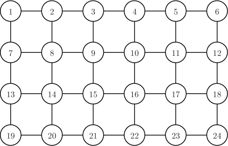
Although it is too small to really be called a small-world network, the network in Figure 12.6 illustrates these ideas. The graph contains three clusters of nodes, centered around nodes 5, 12 and 18, that are connected by a few shortcut links (e.g., the links between nodes 5 and 18 and between nodes 14 and 23). These two characteristics together give an average distance between nodes of about 2.42. On the other hand, the highly structured grid or mesh network in Figure 12.7 has an average node distance of about 3.33. Both of these graphs have 24 nodes and 38 links, so they are both sparse relative to the (24 · 23)/2 = 276 possible links that they could have.
Clustering coefficients
The extent to which the neighborhood of a node is clustered is measured by its local clustering coefficient. The local clustering coefficient of a node is the number of links between its neighbors, divided by the total number of possible links between neighbors. For example, consider the cluster on the left below surrounding the blue node in the center.
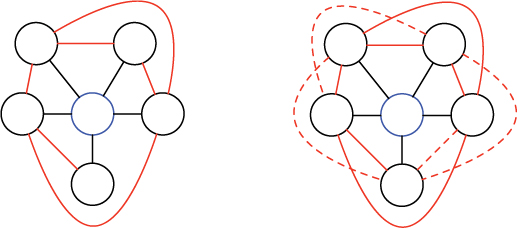
The blue node has five neighbors, with six links between them (in red). Notice that each of these links, together with two black links, forms a closed cycle, called a triangle. So we can also think about the local clustering coefficient as counting these triangles. As shown on the right, there are four dashed links between neighbors of the blue node (i.e., four additional triangles) that are not present on the left, for a total of ten possible links altogether. So the local clustering coefficient of the blue node is 6/10 = 0.6. (The clustering coefficient will always be between 0 and 1.)
Reflection 12.15 In general, if a node has k neighbors, how many possible links are there between pairs of these neighbors?
Each of the k neighbors could be connected to k – 1 other neighbors, for a total of k(k – 1) links. However, this counts each link twice, so the total number of possible links is actually k(k – 1)/2. Therefore, the local clustering coefficient of a node with k neighbors is the number of neighbors that are connected, divided by k(k – 1)/2. The clustering coefficient for an entire network is the average local clustering coefficient over all nodes in the network. The highly structured grid or mesh graph in Figure 12.7 does not have any triangles at all, so its clustering coefficient is 0. On the other hand, the graph in Figure 12.6 has a clustering coefficient of about 0.59.
Reflection 12.16 If you had a small local clustering coefficient in your social network (i.e., if your friends are not friends with each other), what implications might this have?
It has been suggested that situations like this breed instability. Imagine that, instead of a social network, we are talking about a network of nations and links represent the existence of diplomatic relations. A nation with diplomatic relations with many other nations that are enemies of each other is likely in a stressful situation. It might be helpful to detect such situations in advance to curtail potential conflicts.
To compute the local clustering coefficient for a node, we need to iterate over all of the node’s neighbors and count for each one the number of links between it and the other neighbors of the node. Then we divide this number by the maximum possible number of links between the node’s neighbors. This is accomplished by the following function.
def clusteringCoefficient(network, node):
    """Compute the local clustering coefficient for a node.

    Parameters:
        network: a graph represented by a dictionary
        node: a node in the network

    Return value: the local clustering coefficient of node
    """

    neighbors = network[node]
    numNeighbors = len(neighbors)
    if numNeighbors <= 1:
        return 0
    numLinks = 0
    for neighbor1 in neighbors:
        for neighbor2 in neighbors:
            if neighbor1 != neighbor2 and neighbor1 in network[neighbor2]:
                numLinks = numLinks + 1
    return numLinks / (numNeighbors * (numNeighbors - 1))
This function is relatively straightforward. The two for loops iterate over every possible pair of neighbors, and the if statement checks for a link between unique neighbors. However, this process effectively counts every link twice, so at the end we divide by numNeighbors * (numNeighbors - 1) (i.e., k(k – 1)), which is twice what we discussed previously.
Reflection 12.17 Do you see why the function counts every link twice? How can we fix this?
The function effectively counts every link twice because it checks whether each neighbor is in every other neighbor’s list of adjacent nodes. Therefore, for any two connected neighbors, call them A and B, we are counting the link once when we see A in the list of adjacent nodes of B and again when we see B in the list of adjacent nodes of A.
To count each link just once, we can use the following trick. In the list of neighbors, we first check whether the node at index 0 is connected to nodes at indices 1, 2, ..., k – 1. Then, to prevent counting a link twice, we never want to check whether any node is connected to node 0 again. So we next check whether node 1 is connected to nodes 2, 3, ..., k – 1. Now, to prevent double counting, we never want to check whether any node is connected to nodes 0 or 1. So we next check whether node 2 is connected to nodes 3, 4, ..., k – 1. Do you see the pattern? In general, we only want to check whether node i is connected to nodes i + 1, i + 2, ..., k – 1. (This is the same trick you may have seen in Exercise 8.5.4.) This is implemented in the following improved version of the function.
def clusteringCoefficient(network, node):
    """ (docstring omitted) """

     neighbors = network[node]
     numNeighbors = len(neighbors)
     if numNeighbors <= 1:
         return 0
     numLinks = 0
     for index1 in range(len(neighbors) - 1):
         for index2 in range(index1 + 1, len(neighbors)):
             neighbor1 = neighbors[index1]
             neighbor2 = neighbors[index2]
             if neighbor1 != neighbor2 and neighbor1 in network[neighbor2]:
                 numLinks = numLinks + 1
     return numLinks / (numNeighbors * (numNeighbors - 1) / 2)
Once we have this function, to compute the clustering coefficient for the network, we just have to call it for every node, and compute the average. We leave this, and writing a function to compute the average distance, as exercises.
Scale-free networks
In addition to having short paths and high clustering, researchers soon discovered that most small-world networks also contain a few highly connected (i.e., high degree) nodes called hubs that facilitate even shorter paths. In the network in Figure 12.6, nodes 5, 12, and 18 are hubs because their degrees are large relative to the other nodes in the network.
Reflection 12.18 How do connected hubs facilitate short paths?
The existence of hubs in a large network can be seen by plotting for each node degree in the network the fraction of the nodes that have that degree. This is called the degree distribution of the network. The degree distribution for a network with a few hubs will show the vast majority of nodes having relatively small degree and just a few nodes having very large degrees. For example, Figure 12.8 shows such a plot for a small portion of the web. Each node represents a web page and a directed link from one node to another represents a hyperlink from the first page to the second page.1 In this network, 99% of the nodes have degree at most 25, while just a few have degrees that are much higher. (In fact, 98% of the nodes have degrees at most 20 and 90% have degrees at most 15.) These few hubs with high degree enable a small average distance and a clustering coefficient of about 0.37.

Reflection 12.19 In the web network from Figure 12.8, the degree of a node is the number of hyperlinks from that page. How do you think the degree distribution might change if we instead counted the number of hyperlinks to each page?
Networks with this characteristic shape to their degree distributions are called scale-free networks. The name comes from the observation that the fraction of nodes with degree d is roughly (1/d)a, for some small value of a. Such functions are called “scale-free” because their plots have the same shape regardless of the scale at which you view them. A scale-free degree distribution is very different from the normal distribution that seems to describe most natural phenomena, which is why this discovery was so interesting.
Reflection 12.20 How could recognizing that a network is scale-free and then identifying the hubs have practical importance?
The presence of hubs in a network is a double-edged sword. On the one hand, hubs enable efficient communication and transportation. For this reason, the Internet is structured in this way, as are airline networks (see Figure 12.9). Also, because so many of the nodes in a scale-free network are relatively unimportant, scale-free networks tend to be very robust when subjected to random attacks or damage. Some have speculated that, because some natural networks are scale-free, they may represent an evolutionary advantage. On the other hand, because the few hubs are so important, a directed attack on a hub can cause the network to fail. (Have you ever noticed the havoc that ensues when an airline hub is closed due to weather?) A directed attack on a hub can also be advantageous if we want the network to fail. For example, if we suspect that the network through which an epidemic is traveling is scale-free, we may have a better chance of stopping it if we vaccinate the hubs.
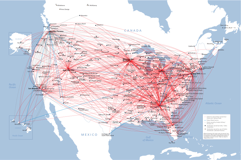
Figure 12.9 The North American routes of Delta Airlines. [9]
Exercises
12.3.1. Write a function that returns the average local clustering coefficient for a network. Test your function by calling it on some of the networks on the book web site. You will need the function assigned in Exercise 12.1.8 to read these files.
12.3.2. Write a function that returns the average distance between every pair of nodes in a network. If two nodes are not connected by a path, assign their distance to be equal to the number of nodes in the network (since this is longer than any possible path). Test your function by calling it on some of the networks on the book web site. You will need the function assigned in Exercise 12.1.8 to read these files.
12.3.3. The closeness centrality of a node is the total distance between it and all other nodes in the network. By this measure, the node with the smallest value is the most central (and perhaps most influential) node in the network. Write a function that computes the closeness centrality of a node. Your function should take two parameters: the network and a node. Test your function by calling it on some of the networks on the book web site. You will need the function assigned in Exercise 12.1.8 to read these files.
12.3.4. Using the function you wrote in the previous exercise, write another function that returns the most central node in a network (with the smallest closeness centrality).
12.3.5. Write a function that plots the degree distribution of a network, producing a plot like that in Figure 12.8. Test your function on a small network first. Then call your function on the large Facebook network (with 4,039 nodes and 88,234 links) that is available on the book web site. (You will need the function assigned in Exercise 12.1.8 to read these files.) Is the network scale-free?
12.4 RANDOM GRAPHS
Since small-world and scale-free networks seem to be so common, it is natural to ask whether such networks just happen randomly. To answer this question, we can compare the characteristics of these networks to a class of randomly generated graphs. In particular, we will look at the class of uniform random graphs, which are created by adding each possible edge with some probability p.
Creating a uniform random graph is straightforward. We first create an adjacency list with the desired number of nodes, then iterate over all possible pairs of nodes. For each pair of nodes, we link them with probability p, as shown below.
import random

def randomGraph(n, p):
    '''Return a uniform random graph with n vertices.

    Parameters:
        n: the number of nodes
        p: the probability that two nodes are connected

    Return value: a random graph
    '''

    graph = { }
    for node in range(n):            # label nodes 0, 1, ..., n-1
        graph[node] = [ ]            # graph has n nodes, 0 links

    for node1 in range(n - 1):
        for node2 in range(node1 + 1, n):
            if random.random() < p:
                graph[node1].append(node2)  # add edge between
                graph[node2].append(node1)  #   node1 and node2
    return graph
Because we will get a different random graph every time we call this function, any characteristics that we want to measure will have to be averages over several different random graphs with the same values of n and p. To illustrate, let’s compute the average distance, clustering coefficient, and degree distribution for uniform random graphs with the same number of nodes and links as the graphs in Figures 12.6 and 12.7. Recall that those graphs had 24 nodes and 38 links.
Reflection 12.21 What parameters should we use to create a uniform random graph with 24 nodes and 38 links?
We cannot specify the number of links specifically in a uniform random graph, but we can set the probability so that we are likely to get a particular number, on average, over many trials. In particular, we want 38 out of a possible (24 · 23)/2 links, so we set
Averaging over 20,000 uniform random graphs, each generated by calling randomGraph(24, 0.14), we find that the average distance between nodes is about 4.32 and the average clustering coefficient is about 0.12. The table below compares these results to what we computed previously for the other two graphs.
Graph |
Average distance |
Clustering coefficient |
Figure 12.6 (clusters) |
2.42 |
0.59 |
Figure 12.7 (grid) |
3.33 |
0 |
Uniform random |
4.32 |
0.12 |
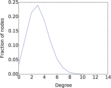
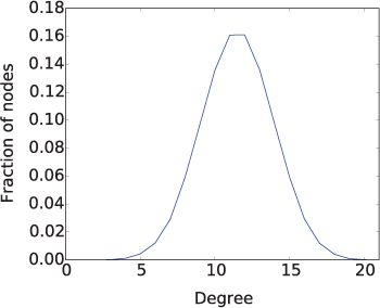
The random graph with the same number of nodes and edges has a slightly longer average distance and a markedly smaller clustering coefficient than the graph in Figure 12.6 with the three clusters. Because these graphs are so small, these numbers alone, while suggestive, are not very strong evidence that random graphs do not have the small-world or scale-free properties. So let’s also look at the average degree distribution of the random graphs, shown in Figure 12.10. The shape of the degree distribution is quite different from that of a scale-free network, and is much closer to a normal distribution. Because the probability of adding an edge was relatively low, the average degree was only about 3 and there were a number of nodes with 0 degree, causing the plot to “run into” the y-axis. If we perform the same experiment with p = 0.5, as shown in Figure 12.11, we get a much clearer bell curve. These distributions show that random graphs do not have hubs; instead, the nodes all tend to have about the same degree. So there is definitely something non-random happening to generate scale-free networks.
Reflection 12.22 What kind of process do you think might create a scale-free network with a few high-degree nodes?
The presumed process at play has been dubbed preferential attachment or, colloquially the “rich get richer” phenomenon. The idea is relatively intuitive: popular people, destinations, and web pages tend to get more popular over time as word of them moves through the network.
Exercises
12.4.1. Show how to create a uniform random graph with 30 nodes and 50 links, on average.
12.4.2. Exercise 12.3.1 asked you to write a function that returns the clustering coefficient for a graph. Use this function to write another function
avgCCRandom(n, p, trials)
that returns the average clustering coefficient, over the given number of trials, of random graphs with the given values of n and p.
12.4.3. Exercise 12.3.2 asked you to write a function that returns the average distance between any two nodes in a graph. Use this function to write another function
avgDistanceRandom(n, p, trials)
that returns the average of this value, over the given number of trials, for random graphs with the given values of n and p.
12.4.4. Exercise 12.3.5 asked you to write a function to plot the degree distribution of a graph and then call the function on the large Facebook network on the book web site. This network has 4,039 nodes and 88,234 links. To compare the degree distribution of this network to a random graph of the same size, write a function
degreeDistributionRandom(n, p, trials)
that plots the average degree distribution, over the given number of trials, of random graphs with the given values of n and p. Then use this function to plot the degree distribution of random graphs with 4,039 nodes and an average of 88,234 links. What do you notice?
12.4.5. We say that a graph is connected if there is a path between any pair of nodes. Random graphs that are generated with a low probability p are unlikely to be connected, while random graphs generated with a high probability p are very likely to be connected. But for what value of p does this transition between disconnected and connected graphs occur?
To determine whether a graph is connected, we can use either a breadth-first search (as in Exercise 12.2.5) or a depth-first search (as in Exercise 12.2.6). In either case, we start from any node in the network, and try to visit all of the other nodes. If the search is successful, then the graph must be connected. Otherwise, it must not be connected.
- Write a function
connectedRandom(n, minp, maxp, stepp, trials)
that plots the fraction of random graphs with n nodes that are connected for values of p ranging from
minptomaxp, in increments ofstepp. To compute the fraction that are connected for each value of p, generatetrialsrandom graphs and count how many of those are connected using yourconnectedfunction from either Exercise 12.2.5 or Exercise 12.2.6. - For n = 24, what do you find? For what value of p is there a 50% chance that the graph will be connected? Does the transition from disconnected graphs to connected graphs happen gradually or is change abrupt?
12.5 SUMMARY
In this chapter, we took a peek at one of the more exciting interdisciplinary areas in which computer scientists have become engaged. Networks are all around us, some obvious and some not so obvious. But they can all be described using the language of graphs. The shortest path and distance between any two nodes in a graph can be found with the breadth-first search algorithm. Graphs in which the distance between any two nodes is relatively short and the clustering coefficient is relatively high are called small-world networks. Networks that are also characterized by a few high-degree hubs are called scale-free networks. Scientists have discovered over the last two decades that virtually all large-scale natural and human-made networks are scale-free. Knowing this about a network can give a lot of information about how the network works and about its vulnerabilities.
12.6 FURTHER DISCOVERY
This chapter’s epigraph is from a 1967 article by Stanley Milgram titled, The Small-World Problem [33]. Dr. Milgram was an influential American social psychologist. Besides his small world experiment, he is best known for experiments in which he demonstrated that ordinary people are capable of disregarding their consciences when instructed to do so by those in authority.
There are several excellent books for a general audience about the emerging field of network science. Three of these are Six Degrees by Duncan Watts [57], Sync by Steven Strogatz [54], and Linked by Albert-László Barabási [3]. Think Complexity by Allen Downey [10] introduces slightly more advanced material on implementing algorithms on graphs, small-world networks, and scale-free networks in Python.
12.7 PROJECTS
Project 12.1 Diffusion of ideas and influence
In this project, you will investigate how memes, ideas, beliefs, and information propagate through social networks, and who in a network has the greatest influence. We will simulate diffusion through a network with the independent cascade model. In this simplified model, an idea originates at one node (called the seed) and each of the neighbors of this node adopts it with some fixed probability (called the propagation probability). This probability measures how influential each node is. In reality, of course, people have different degrees of influence, but we will assume here that everyone is equally influential. Once the idea has propagated to one or more new nodes, each of these nodes gets an opportunity to propagate it to each of their neighbors in the next round. This process continues through successive rounds until all of the nodes that have adopted the idea have had a chance to propagate it to their neighbors.
For example, suppose node 1 in the network below is the seed of an idea.

In round 1, node 1 is successful in spreading the idea to node 2, but not to node 4. In round 2, the idea spreads from node 2 to both node 3 and node 5. In round 3, the idea spreads from node 3 to node 7, but node 3 does not successfully influence node 8. Node 5 also attempts to influence node 4, but is unsuccessful. In round 4 (not shown), node 7 attempts to spread the idea to nodes 6 and 8, but is unsuccessful, and the process completes.
Part 1: Create the network
For this project, you will use a network that is an anonymized version of a very small section of the Facebook network with 333 nodes and 2,519 links. The file containing this network is available on the book web site. The format of the file is the same as the format described in Exercise 12.1.8: each node is represented by a number, and each line represents one link. If you have not already done so in Exercise 12.1.8, write a function
readNetwork(fileName)
that reads in a network file with this format, and returns an adjacency list representation of the network.
Part 2: Simulate diffusion with a single seed
Simulating the diffusion of an idea through the network, as described above, is very similar to a breadth-first search, except that nodes are visited probabilistically. Just as visited nodes are not revisited in a BFS, nodes that have already adopted the idea are not re-influenced. Using the bfs function from Section 12.2 as a starting point, write a function
diffusion(network, seed, p)
that simulates the independent cascade model starting from the given seed, using propagation probability p. The function should return the total number of nodes in the network who adopted the idea (i.e., were successfully influenced).
Part 3: Rate each node’s influence
Because this is a random process, the diffusion function will return a different number every time it is run. To get a good estimate of how influential a node is, you will have to run the function many times and average the results. Therefore, write a function
rateSeed(network, seed, p, trials)
that calls diffusion trials times with the given values of network, seed and p, and returns the average number of nodes influenced over that many trials.
Part 4: Find the most influential node(s)
Finally, write a function
maxInfluence(network, p, trials)
that calls the rateSeed function for every node in the network, and returns the most influential node.
Combine these functions into a complete program that finds the most influential node(s) in the small Facebook network, using a propagation probability of 0.05. Then answer the following questions. You may write additional functions if you wish.
Question 12.1.1 Which node(s) turned out to be the most influential in your experiments?
Question 12.1.2 Were the ten most influential nodes the same as the ten nodes with the most friends?
Question 12.1.3 Can you find any relationship between a person’s number of friends and how influential the person is?
Project 12.2 Slowing an epidemic
In Section 4.4, we simulated the spread of a flu-like virus through a population using the SIR model. In that simulation, we lumped all individuals into three groups: those who are susceptible to the infection, those who are currently infected, and those who recovered. In reality, of course, not every individual in the susceptible group is equally susceptible and not every infected person is equally likely to infect others. Some of the differences have to do with who comes into contact with whom, which can be modeled by a network. For example, consider the network in Figure 12.6 on Page 602. In that network, if node 3 becomes infected and there is a 10% chance of any individual infecting a contact, then the virus is very unlikely to spread at all. On the other hand, if node 12 becomes infected, there is a 9 · 10% = 90% chance that the virus will spread to at least one of the node’s nine neighbors.
If a vaccine is available for the virus, then knowledge about the network of potential contacts can be extremely useful. In this project, you will simulate and compare two different vaccination strategies: vaccinating randomly and vaccinating targeted nodes based on a criterion of your choosing.
Part 1: Create the network
For this project, you will use a network that is an anonymized version of a very small section of the Facebook network with 333 nodes and 2,519 links. The file containing this network is available on the book web site. The format of the file is the same as the format described in Exercise 12.1.8: each node is represented by a number, and each line represents one link. If you have not already done so in Exercise 12.1.8, write a function
readNetwork(fileName)
that reads in a network file with this format, and returns an adjacency list representation of the network.
Part 2: Simulate spread of the contagion through the network
Simulating the spread of the infection through the network is very similar to a breadth-first search, except that nodes are visited (infected) probabilistically and we will assume that each infection starts with a random source node. Once a node has been infected, it should be enqueued so that it has an opportunity to infect other nodes. When a node is dequeued, it should attempt to infect all of its uninfected neighbors, successfully doing so with some infection probability p. But once infected, a node should never be infected again or put back into the queue. Using the bfs function from Section 12.2 as a starting point, write a function
infection(network, p, vaccinated)
that simulates this infection spreading in network, starting from a randomly chosen source node, and using infection probability p. The fourth parameter, vaccinated, is a list of nodes that are immune to the infection. An immune node should never become infected, and therefore cannot infect others either; more on this in Part 3. The function should return when all infected nodes have had a chance to infect their neighbors. The function should return the total number of nodes who were infected.
Part 3: Simulate vaccinations
Now, you will investigate how the number of infected nodes is affected by vaccinations. Assume that the number of vaccine doses is limited, and compare two different strategies for choosing the sequence of nodes to vaccinate. For each strategy, first run your simulation with no vaccinations, then with only the first node vaccinated, then with the first two nodes vaccinated, etc. Because the infection is a random process, each simulation with a different number of vaccinations needs to be repeated many times to find an average number of infected nodes.
First, investigate what happens if you vaccinate a sequence of random nodes. Second, design a better strategy, and compare your results to the results of the random vaccinations. Use the ideas from this chapter to learn about the network, and choose a specific sequence of nodes that you think will do a better job of reducing the number of infections in the network.
Implement these simulations in a function
vaccinationSim(network, p, trials, numVaccs, randomSim)
If the last parameter randomSim is True, the function should perform the simulation with random vaccinations. Otherwise, it should perform the simulation with your improved strategy. The fourth parameter, numVaccs, is the number of individuals to vaccinate. For every number of vaccinations, the simulation should call the infection function trials times with the given network and infection probability p. The function should return a list of numVaccs + 1 values representing the average number of infections that resulted with 0, 1, 2, ..., numVaccs immune nodes.
Create a program that calls this function once for each strategy with the following arguments:
infection probability 0.1
500 trials
50 vaccinations
Then your program should produce a plot showing for both strategies how the number of infections changes as the number of vaccinations increases.
Question 12.2.1 What strategy did you choose?
Question 12.2.2 Why did you think that your strategy would be effective?
Question 12.2.3 How successful was your strategy in reducing infections, compared to the random strategy?
Question 12.2.4 Given an unlimited number of vaccinations, how many are required for the infection to not spread at all?
Project 12.3 The Oracle of Bacon
In the 1990’s, a group of college students invented a pop culture game based on the six degrees of separation idea called the “Six Degrees of Kevin Bacon.” In the game, players take turns challenging each other to identify a connected chain of actors between Kevin Bacon and another actor, where two actors are considered to be connected if they appeared in the same movie. An actor’s Bacon number is the distance of the actor from Kevin Bacon.
This game later spawned the “Oracle of Bacon” website, at http://oracleofbacon.org, which gives the shortest chain between Mr. Bacon and any other actor you enter. This works by constructing a network of actors from the Internet Movie Database (IMDb)2, and then using breadth-first search to find the desired path. This network of movie actors provides fertile ground for investigating all of the concepts discussed in this chapter. Is the network really a small-world network, as suggested by the “Six Degrees of Kevin Bacon?” Is there really anything special about Kevin Bacon in this network? Or is there a short path between any two pair of actors? Is the network scale-free?
In this project, you will create an actor network, based on data from the IMDb, and then answer questions like these. You will also create your own “Oracle of Bacon.”

Part 1: Create the network
On the book web site, you will find several files, created from IMDb database files, that have the following format:
League of Their Own, A (1992)Tom Hanks
Animal House (1978)
Apollo 13 (1995)
The files are tab-separated (the ![]() symbols represent tabs). The first entry on each line is the name of a movie. The movie is followed by a list of actors that appeared in that movie.
symbols represent tabs). The first entry on each line is the name of a movie. The movie is followed by a list of actors that appeared in that movie.
Write a function
createNetwork(filename)
that takes the name of one of these data files as a parameter, and returns an actor network (as an adjacency list) in which two actors are connected if they have appeared in the same movie. For example, for the very short file above, the network would look like that in Figure 12.12. Each link in this network is labeled with the name of a movie in which the two actors appeared. This is not necessary to determine a Bacon number, but it is necessary to display all the relationships, as required by the traditional “Six Degrees of Kevin Bacon” game (more on this later).
The following files were created from the IMDb data, and are available on the book web site.
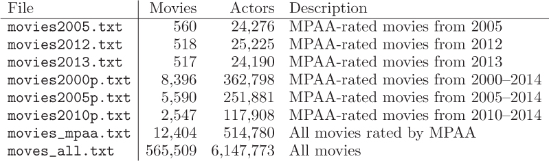
Start by testing your function with the smaller files, building up to working with the entire database. Keep in mind that, when working with large networks, this and your other functions below may take a few minutes to execute. For each file, we give the number of movies, the total number of actors in all casts (not unique actors), and a description.
Part 2: Is the network scale-free?
Because the actor network is so large, it will take too much time to compute the average distance between its nodes and its clustering coefficient. But we can plot the degree distribution and investigate whether the network is scale-free. To do so, write a function
degreeDistribution(network)
that plots the degree distribution of a network using matplotlib. Again, start with small files and work your way up.
Question 12.3.1 What does your plot show? Is the network scale-free?
Question 12.3.2 Where does Kevin Bacon fall on your plot? Is he a hub? If so, is he unique in being a hub?
Question 12.3.3 Which actors have the ten largest degrees? (They might not be who you expect.)
Part 3: Oracle of Bacon
You now know everything you need to create your own “Oracle of Bacon.” Write a function
oracle(network)
that repeatedly prompts for the names of two actors, and then prints the distance between them in the network. Your function should call bfs to find the shortest distance.
For an extra challenge, modify the algorithm (and your adjacency list) so that it also prints how the two actors are related. For example, querying the oracle with Kevin Bacon and Zooey Deschanel might print
Zooey Deschanel and Kevin Bacon have distance 2.

1. Kevin Bacon was in "The Air I Breathe (2007)" with Clark Gregg.
2. Clark Gregg was in "(500) Days of Summer (2009)" with Zooey Deschanel.
Part 4: Frequencies of Bacon numbers
Finally, determine just how central Kevin Bacon is in the movie universe. To do so, create a chart with the frequency of Bacon numbers. Write a function
baconNumbers(network)
that displays this chart for the given network. For example, given the file movies2013.txt, your function should print the following:
Bacon Number     Frequency
------------     ---------
     0                   1
     1                 152
     2                2816
     3               12243
     4                4230
     5                 253
     6                  47
     7                   0
     8                   0
  infinity             819
An actor has infinite Bacon number if he or she cannot be reached from Kevin Bacon.
Once your function is working, call it with some of the larger files.
Question 12.3.4 What does the chart tell you about Kevin Bacon’s place in the movie universe?
1Web network data obtained from http://snap.stanford.edu/data/web-Google.html